At a glance
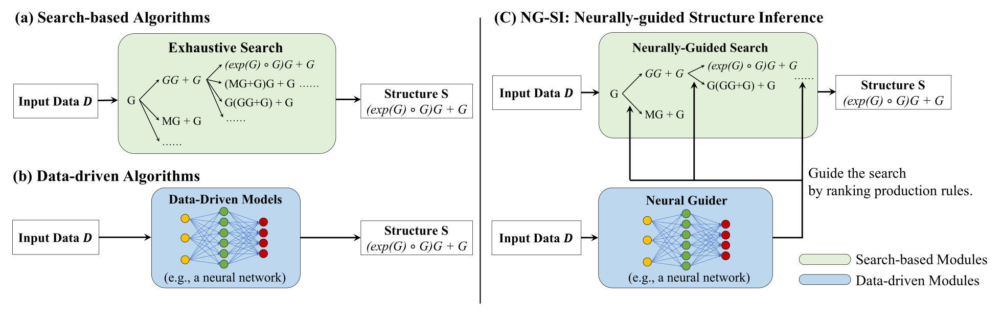
NG-SI uses a neural network to choose grammar rules within a recursive structure-inference procedure. Expert-designed algorithms then decompose the input so the same inference routine can operate on each component. The goal is to avoid evaluating every rule without requiring a neural network to predict an entire deep structure at once.
Experiments cover probabilistic matrix decomposition and parsing a synthetic programming language. The method is faster than the tested search baselines and generalizes better than the tested neural sequence/tree baselines to deeper structures. Its performance still depends on the supplied grammar, decomposition procedures, training distribution, and rule-selection accuracy.
1. Introduction
Many data structures can be expressed by composing a small set of primitives. Exhaustively evaluating candidate structures is expensive, while directly predicting a whole structure can fail outside the training complexity range. NG-SI places learned guidance at each local expansion, preserving the recursive organization of search. Figure 1 contrasts the three approaches.
2. Structure inference
Structure inference jointly seeks an explanatory structure and the parameters associated with it. The paper assumes that a domain-specific grammar and primitive operations are already available.
2.1. Problem formulation
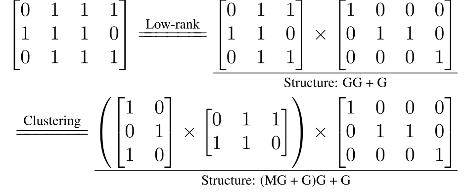
A matrix can, for example, have low-rank structure whose factors themselves exhibit clustering. The grammar expresses such nested structure; terminals describe primitives and production rules combine them. Figure 2 retains the numerical decomposition example.
The task is inference within a supplied language. The algorithm does not discover the language’s primitives or production rules from scratch.
2.2. Prior work
Earlier work spans explicit search, amortized neural prediction, and learned search guidance. The proposed distinction is amortizing rule selection at each level while retaining expert-defined recursive decomposition.
Search-based structure inference
Search-based methods enumerate rule expansions, fit candidate components, and rank structures using a domain-specific score. The matrix method of Grosse et al. [15] supplies both the grammar and decomposition machinery used here. Restricting expansion to good candidates reduces search, but fitting and ranking many alternatives remains expensive.
Data-driven structure inference
Sequence, tree, and program-prediction models learn mappings from labeled examples. They amortize inference but can struggle when test sequences are longer or structures are deeper than training examples. This motivates reusing a local predictor recursively.
Guided search
Prior systems guide search using learned proposals, execution, types, sketches, or learned subroutines. NG-SI instead predicts the next production rule from the current input component and delegates decomposition to a rule-specific algorithm.
3. Neurally-guided structure inference
Algorithm 1 recursively selects a rule, decomposes the input into components corresponding to its nonterminal symbols, and invokes itself on each component. A neural guider implements rule selection. The displayed algorithm is greedy; beam-search extensions are possible but are not the pseudocode shown.
Recursion permits reusing known rules at greater depth. It does not guarantee that the neural guider chooses correctly on arbitrary inputs, or that a greedy choice recovers the globally best structure.
Function Infer(D, Type):
    rule ← SelectRule(D, Type)
    for each non-terminal symbol s in rule do
        C_s ← DecomposeData(D, rule, s)
        Replace s in rule with Infer(C_s, s)
    return rule
4. Matrix decomposition
The first application reuses a probabilistic matrix grammar to infer combinations of low rank, clustering, temporal structure, binary factors, and Gaussian scale mixtures.
4.1. Problem formulation
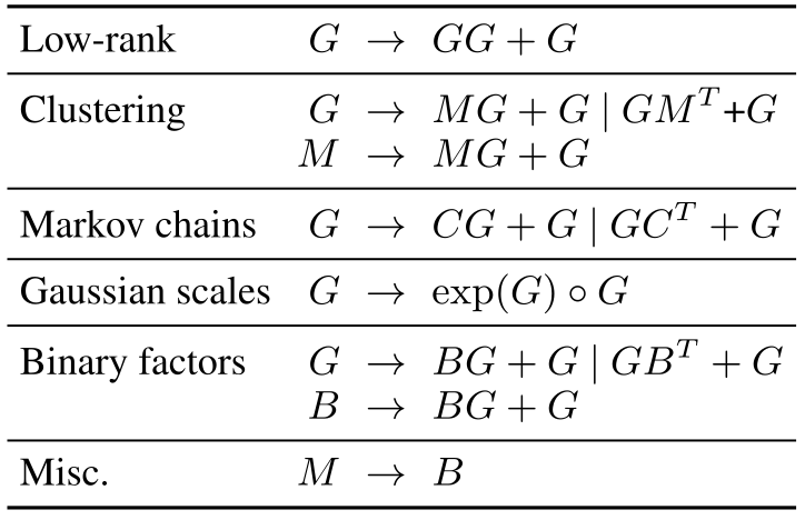
The start symbol G represents an independent Gaussian matrix. Other primitives include multinomial cluster labels M, binary factors B, and cumulative matrices C. Production rules combine these into richer distributions; for example, MG + G describes cluster centers plus Gaussian noise. Table 1 retains the complete grammar, including transpose and elementwise-product notation.
4.2. Method
A convolutional guider recognizes the local pattern associated with each candidate rule. The existing symbolic algorithms fit the selected decomposition, and the existing variational score ranks candidate structures. Thus the speedup concerns choosing and evaluating rules within an inherited inference framework.
Neural guider
The guider predicts local refinements such as low-rank products, row or column clustering, temporal structure, binary factors, or Gaussian scale mixtures. It is trained on rule labels, rather than on complete arbitrarily deep matrix structures.
Training
Training matrices are synthesized online: sample a grammar rule, sample its component matrices, compose them, and use the chosen rule as the target. After training, the guider is fixed during structure inference.
Hyperparameters
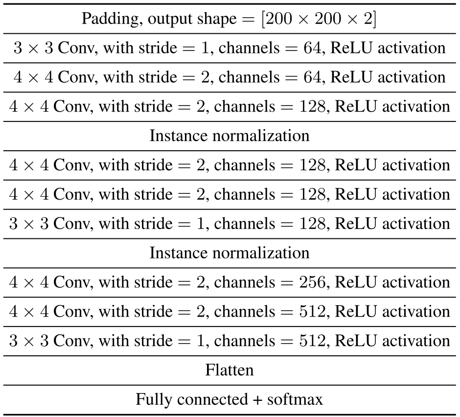
Inputs are described as zero-padded to 200×200 with a second channel marking valid entries. The model trains for 100,000 iterations with batch size 100 and Adam at learning rate 0.0001; the reported decay parameters are both 0.9.
The main text calls the guider eight-layer, while the complete supplementary table lists nine convolutional operations. The original architecture is retained so this discrepancy remains visible.
4.3. Experiments
Synthetic evaluation uses ten matrix structures with 200×200 observations and hidden dimension 10. Real-data examples use walking-motion measurements and natural-image patches, with search depths up to three. The real datasets have no ground-truth structure.
Baselines
The search comparison is the inherited matrix-inference procedure [15]. The learned baseline, Mat2Seq, uses a convolutional encoder and recurrent decoder to generate a full structure, trained on the same synthetic data as the local guider. This design makes extrapolation from local-rule training a central part of the comparison.
Accuracy
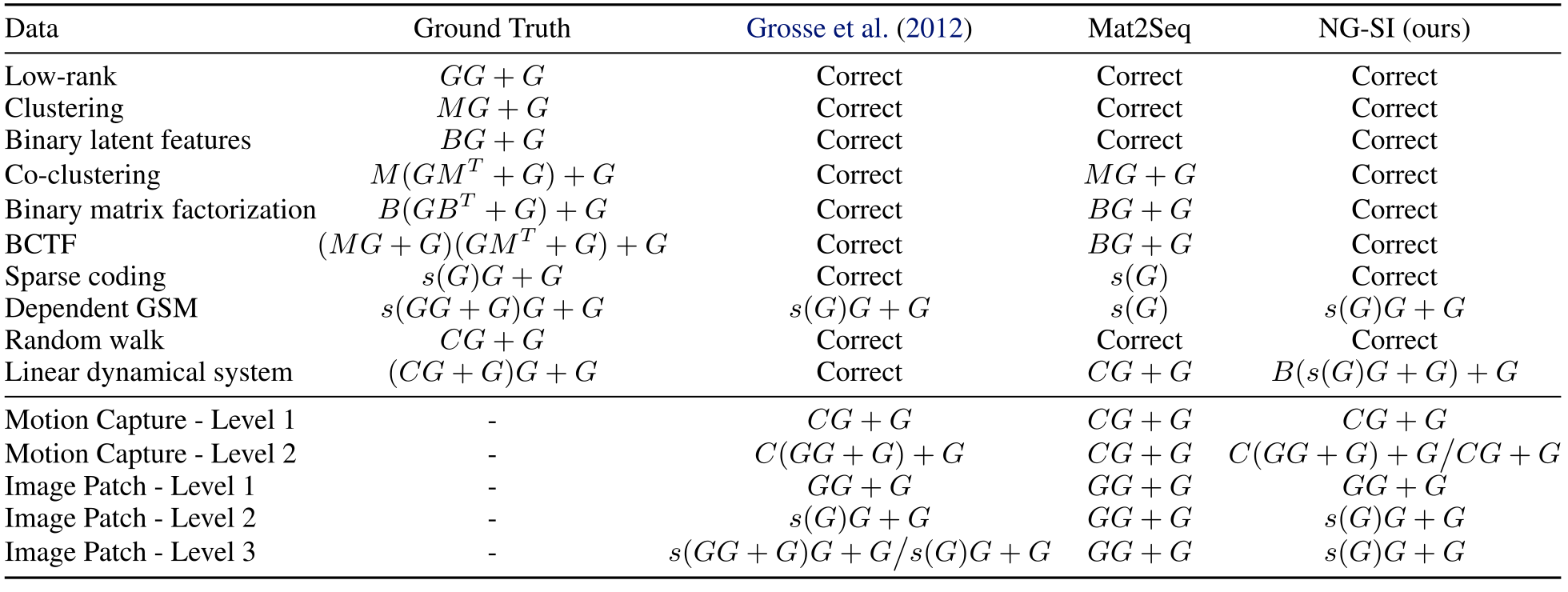
NG-SI recovers eight of the ten tested synthetic structures. It confuses dependent Gaussian scale mixtures with sparse coding, a limitation shared with the variational ranking score, and fails on the linear dynamical-system case. The authors attribute the latter partly to imbalanced training for temporally dependent rules.
On real data, inferred structures mostly agree with the search baseline but can vary across seeds or fall back to simpler structures. Agreement is evidence of consistency with that baseline, not proof of a correct latent structure. Table 2 preserves all reported outcomes across three runs, including disagreements.
Efficiency
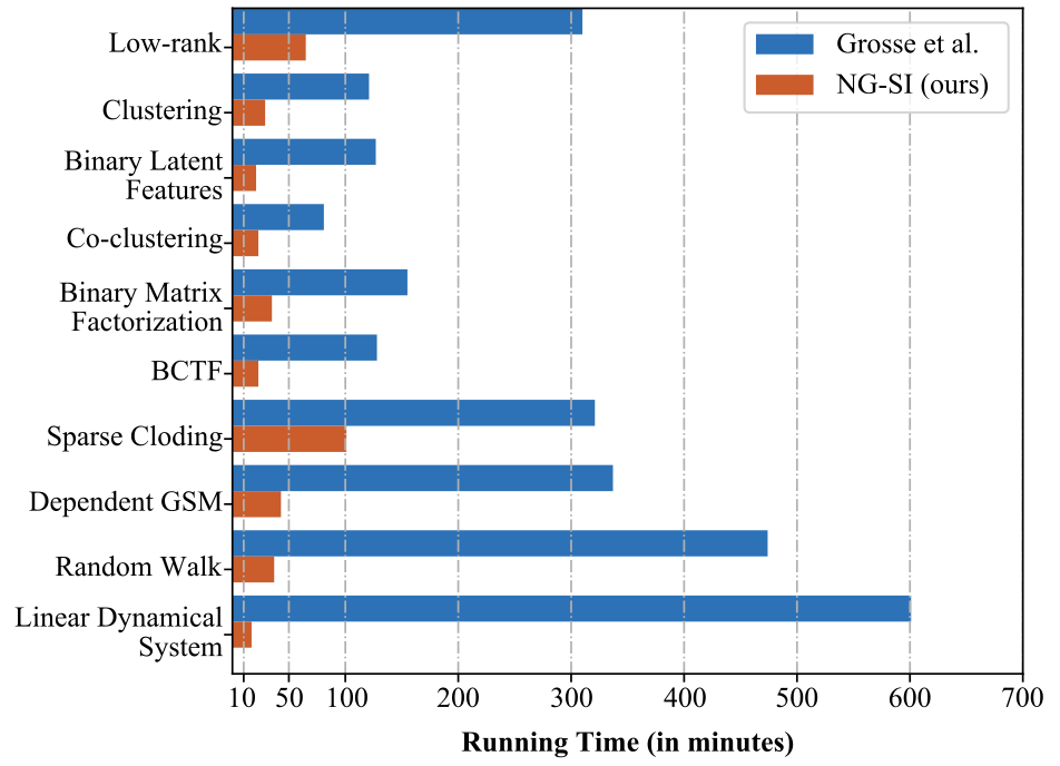
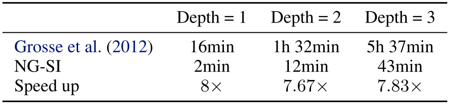
Across the synthetic structures, reported speedups are 3–39×. On a dependent scale-mixture example, depth-one/two/three searches take 2, 12, and 43 minutes versus 16, 92, and 337 minutes for the search baseline, or about 8× faster. Table 3 retains the machine specification and each depth’s timing.
Rule similarity discovery
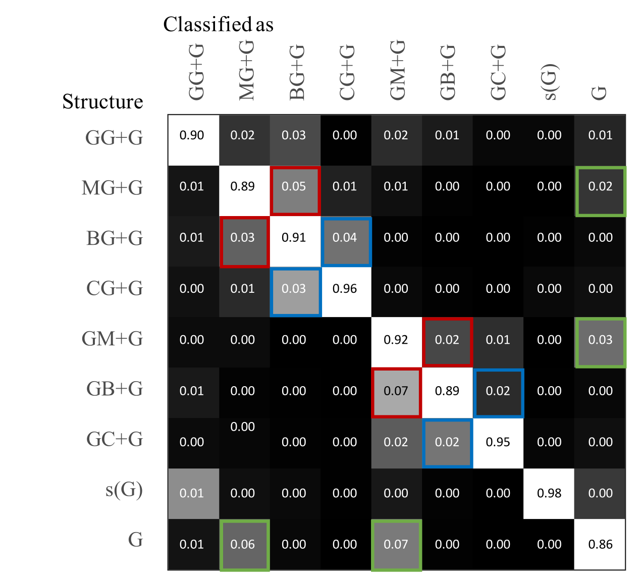
The guider’s average classification probabilities show confusion between structurally related rules, such as clustering and binary factors. Figure 4 preserves the matrix and colored highlights. This is an empirical pattern in learned predictions, rather than a formal metric proving semantic similarity.
4.4. Inspecting GANs
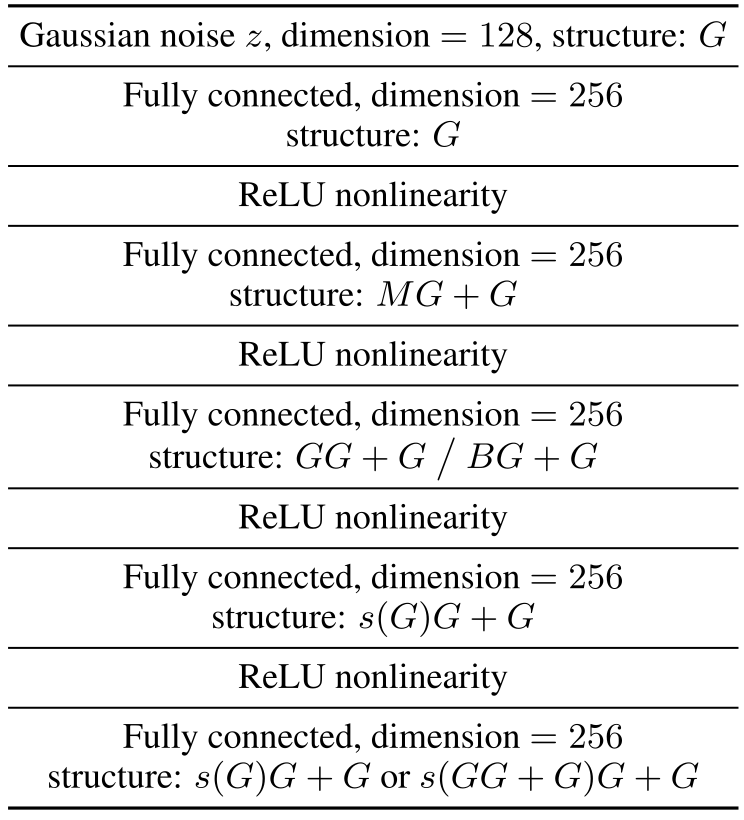
An exploratory example probes intermediate features of a multilayer generative adversarial network trained to produce dependent scale-mixture data. The inferred structures tend to become more elaborate across layers. Table 4 preserves the architecture and alternative inferred structures.
The generator uses a 128-dimensional Gaussian input and 256-dimensional hidden layers, trained for 10,000 generator updates with four discriminator updates per step. This demonstration suggests an interpretive tool; it does not establish that inferred structures uniquely identify how a general GAN computes.
5. Program parsing
The second application maps programs in a synthetic WHILE language into abstract syntax trees. It tests whether learned local rule selection can extrapolate to longer programs and deeper compositions.
5.1. Problem formulation
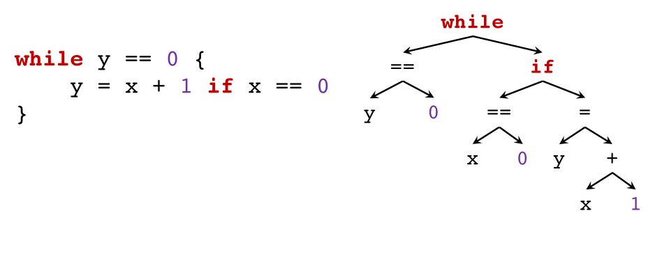
The supplied grammar contains 73 rules covering arithmetic, assignment, conditions, and loops. The input is a program string and the target is its syntax tree. Figure 5 keeps the example program and tree together. This evaluates parsing a known formal language, not discovering program semantics from execution alone.
5.2. Model
A 256-dimensional unidirectional gated recurrent unit encodes the current code string. A linear classifier predicts its top-level rule; hand-coded procedures split the string into the required components, which are parsed recursively. These decomposition routines are important supplied structure.
Training
Programs are generated from the grammar, and every subtree’s corresponding substring becomes a training example. Training limits tree depth to below nine and uses short programs. The task description says length below 15, while the later curriculum description ends at 15; the paper does not reconcile that boundary wording.
Hyperparameters
The parser trains with batch size 64 and Adam at learning rate 0.0001, with both reported decay parameters 0.9. A curriculum increases program length and depth, beginning at length 5 and ending at 15; the full curriculum is repeated three times.
5.3. Experiments
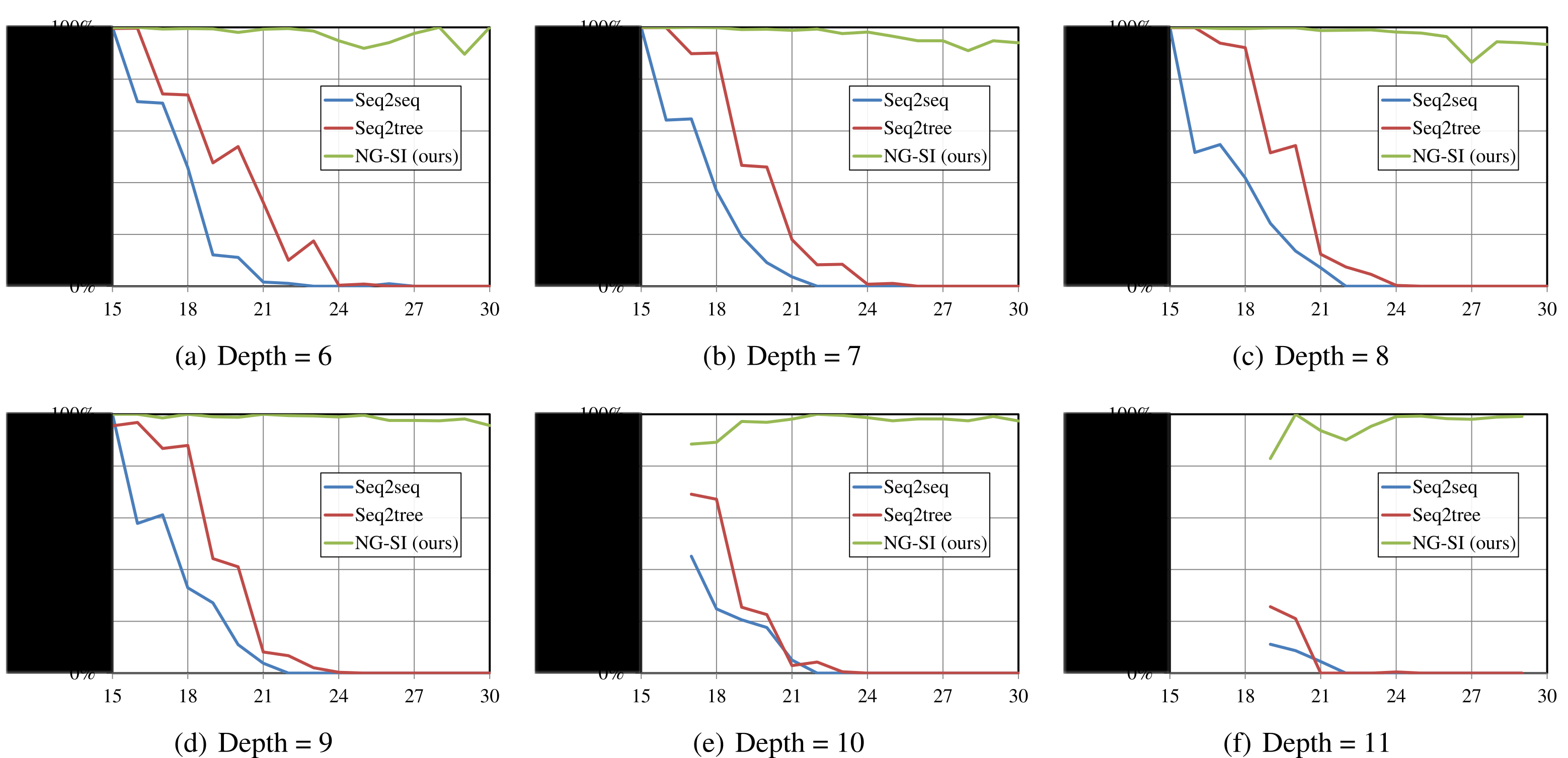
Evaluation varies syntax-tree depth from 6 to 11 and program length from 15 to 30. Very deep trees have a minimum possible length, so not every grid combination is valid.
Baselines
Seq2Seq predicts a preorder serialization of the syntax tree; Seq2Tree expands a tree top-down. Both use attention and 256-dimensional recurrent encoders. Teacher forcing and matching optimizer settings train the neural baselines. An additional search baseline uses iterative-deepening depth-first enumeration until it finds a tree reproducing the input.
Results
NG-SI retains high parsing accuracy across the tested deeper and longer programs, while both neural baselines deteriorate sharply outside training lengths. Figure 6 retains all six depth panels and their individual failure points. The paper’s broad claim of robustness to arbitrary complexity goes beyond this finite test grid.
All three neural methods run in under one second per instance. At fixed depth six, exhaustive search is exact for programs of length at most 24 but exceeds the one-hour limit for longer programs on the reported single-threaded machine.
6. Conclusion
Neural local-rule selection can substantially reduce a structured search’s cost while keeping useful compositional generalization. The evidence covers two supplied grammars and relies on hand-designed decomposition procedures. Incorrect local decisions, distribution imbalance, noisy data, and imperfect ranking scores remain failure modes.
Acknowledgments
The authors thank Xinyun Chen and acknowledge support from the Center for Brains, Minds and Machines, US research funding, and Facebook.
Supplement: neural-guider architecture
The complete supplementary architecture table is retained, including padding, all nine convolutional operations, two normalization stages, flattening, and the final classifier.