At a glance
Passive Interaction Control with Dynamical Systems (PICDS) evaluates a desired velocity field at the robot’s actual position, so physical contact can change the planned motion immediately. Direction-dependent damping rejects motion across the task direction. A conservative field admits a direct passivity proof; a virtual energy tank extends the controller to general fields by limiting energy-producing actions. A plate-insertion experiment illustrates better approach shape and lower contact forces than the tested trajectory-tracking controller. Passivity is the central guarantee, not exact tracking, convergence to the original target during contact, or human safety.
I. Introduction
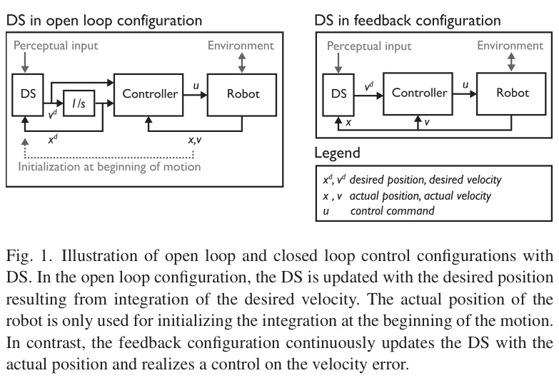
Integrating a dynamical system (DS) into a reference trajectory makes it responsive to sensed target changes but disconnects it from physical disturbances of the robot. Feeding actual position back into the field closes this gap. Conventional impedance tracking can supply energy through its moving reference; passive velocity-field methods instead account for energy explicitly. [10] [12]
The proposed architecture uses selective dissipation rather than continually redirecting all kinetic energy along the task. It combines a task-aligned damping design, conservative-field feedback, an energy-tank extension, and an interpretation of the resulting mechanical impedance. Learning the task field is outside this paper’s scope.
II. Problem statement
The nominal field is known and evaluable, continuous, and has one stable equilibrium. Its integral curves describe desired unperturbed motion. The robot follows the stated rigid-body model with inertia, Coriolis/centrifugal terms, gravity, commanded generalized force, and external generalized force.
The controller should produce a passive relation from external generalized force to velocity, encourage motion along the field, dissipate transverse motion, and permit task-dependent impedance tuning. The paper explicitly does not require closed-loop asymptotic convergence to the field’s attractor: sustained interaction can prevent or make such convergence undesirable. The analysis uses gravity compensation and the mechanical identity that the inertia derivative minus twice the Coriolis matrix is skew-symmetric.
Equation 1

III. Proposed approach
The construction proceeds from passive damping to conservative driving forces and finally to a bounded energy budget for nonconservative motion.
III-A. Selective energy dissipation
The damping matrix uses an orthonormal basis aligned with the desired velocity and nonnegative eigenvalues. With zero damping along the field and positive transverse damping, external motion along the task direction is accepted while sideways kinetic energy is dissipated. This damper alone cannot initiate the desired motion.
Damping remains passive as its orientation or nonnegative gains vary. Near a zero field, the paper retains the preceding basis below a small norm threshold. In the driven controllers, the constant longitudinal gain also scales the potential and driving force; the transverse gains can vary freely while remaining nonnegative.
Equations 2–3


III-B. Tracking conservative fields
For a conservative field, the desired velocity is the negative gradient of a scalar potential. Velocity-error feedback then combines damping with a longitudinal driving force. Because the field is an eigenvector of the damping matrix, its gain is the longitudinal eigenvalue.
Proposition 1 uses robot kinetic energy plus the gain-scaled potential as storage. With a valid lower-bounded potential storage, constant longitudinal gain, and the stated robot model, the derivative equals external power minus damping loss. The potential need not be evaluated by the controller. The result establishes force–velocity passivity; motion accuracy still depends on robot dynamics and the chosen field. Learned SEDS and LMDS fields need not be conservative. [5] [6]
Equations 4–8





III-C. Extension to nonconservative fields
Split the desired field into a conservative component and a residual. A virtual tank stores some energy that damping would otherwise dissipate. Its state is an energy quantity with a finite upper bound; the residual’s power determines whether the tank is charged or spent. Energy tanks were previously used in telemanipulation and variable-stiffness control. [17] [20]
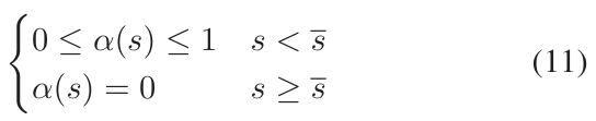
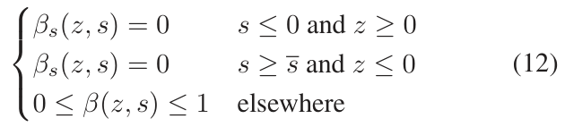
Theorem 1 assumes a positive initial tank level no greater than its cap and coupling functions satisfying Equations (11), (12), and (14). Charging stops at the upper bound, and energy-producing residual action is blocked at depletion. The controller and tank couplings agree when residual power is nonnegative; for negative residual power, the controller coupling may be larger. These conditions make the tank remain bounded and make total storage—kinetic energy, conservative potential energy, and tank energy—increase no faster than external work.
The conservative component remains available when the tank empties, but the desired residual may be suppressed. Thus passivity does not imply unrestricted reproduction of the original field. If no useful conservative component is extracted, depletion can remove the driving motion altogether.
Equations 9–18








III-D. Decomposing the task field
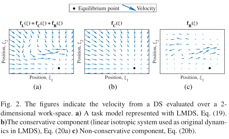
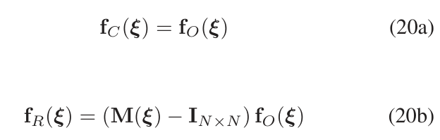
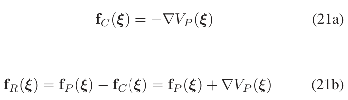
An exact rotational/conservative separation is unnecessary: any conservative component and the remaining difference suffice, including a zero conservative component. A useful component improves behavior after depletion. LMDS reshapes a known original field, so a conservative original field gives the required split directly. For a learned system with a known Lyapunov function, its negative gradient supplies a conservative component and subtraction gives the residual. This also accommodates LMDS built on a SEDS model. [5] [6] [7]
The source’s Equation (20b) labels the modulation matrix M, although Equation (19) calls it G. The original equations are retained.
Equations 19–21

III-E. Impedance adjustment
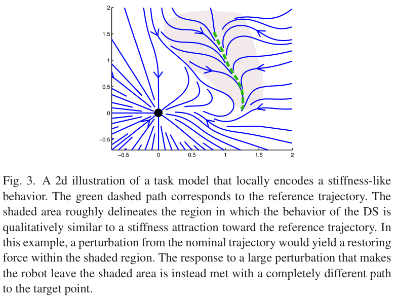
There is a position-dependent desired velocity rather than an independently moving reference position. When the tank does not limit the residual, the closed-loop dynamics combine the physical inertia, damping, and a nonlinear position force. The architecture does not reshape inertia. Transverse damping sets resistance to sideways motion; the longitudinal gain affects the driving force and tracking response.
Near the equilibrium, steady-state linearization gives an effective stiffness equal to minus the longitudinal gain times the field Jacobian. Away from equilibrium, the expansion also contains a nonzero bias force. A generic field therefore does not behave like a symmetric spring around one prescribed trajectory. If local attraction back to a path is desired, that behavior must be encoded in the field; larger perturbations may legitimately follow another integral curve.
Equations 22–24



IV. Robot experiment
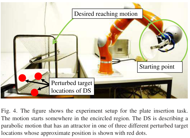
The hardware task inserts a plate into a dish rack whose location differs from the modeled target. Demonstrations produce an LMDS model reshaping a SEDS field; the conservative component is extracted as described above. The desired approach is parabolic. The evaluation compares two controllers on this one manipulation task.
IV-A. Experimental setup
Three target offsets place the modeled attractor behind the actual rack. Each offset is tested five times per controller. Controller A uses the tank controller with initial level and cap both 10, longitudinal gain 20, and both transverse gains 200. Controller B integrates the field from the initial position and tracks the resulting trajectory with an impedance controller using isotropic stiffness 100 and no inertia shaping.
The gains were chosen as low as practicable for each controller: A must overcome initial static friction and B must reach the target in free motion. Both start in a small region, use strong rotational damping of 4 N·s/rad, and omit inverse-dynamics control. These choices favor compliance over precise tracking.
IV-B. Results
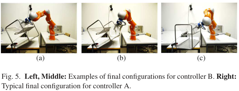
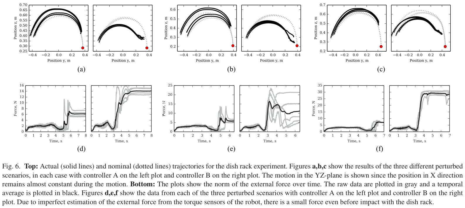
Both controllers deviate from the nominal trajectory. Controller A better preserves the approach shape and consistently places the plate correctly in the reported three offset conditions. Controller B tends to take shortcuts, sometimes leaving the plate on or under the rack. Its integrated reference has already reached the final point at impact, creating a position error that can sustain substantial contact force.
The plotted force traces are lower for A than B after contact in these tests. High transverse damping helps reject unwanted motion, while outcome and tracking quality remain gain-dependent. Force estimates have a small pre-contact bias from imperfect torque-based estimation. This is a small, task-specific comparison; the paper provides trajectories and force traces rather than a broad benchmark or statistical generalization claim.
V. Discussion
Closing the feedback loop lets the task model react to contact while the energy analysis supports interaction with passive environments under the stated assumptions. That guarantee does not bound every hazardous force or make human interaction safe: the field, speed, gains, implementation, and environment still matter.
Compared with power-preserving velocity-field controllers, selective damping deliberately discards unwanted energy instead of retaining and redirecting it. Compared with passivity-preserving speed regulation along one trajectory, a field can describe many alternative paths. Earlier tank methods remain relevant; the new contribution is their integration with this task-dependent velocity feedback. [12] [13] [14] [21]
Tank capacity and initialization are important task choices because unknown disturbances can exhaust the budget and degrade the intended motion. Learning an appropriate energy allowance from supervision is proposed future work. The study does not establish accurate tracking or target convergence for arbitrary contact and depletion histories.
Appendix A. Smooth coupling functions
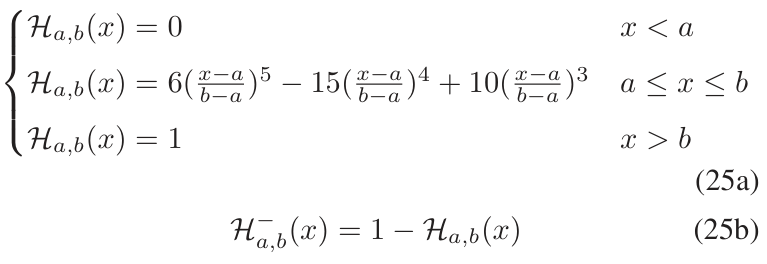
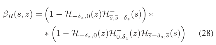
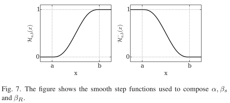
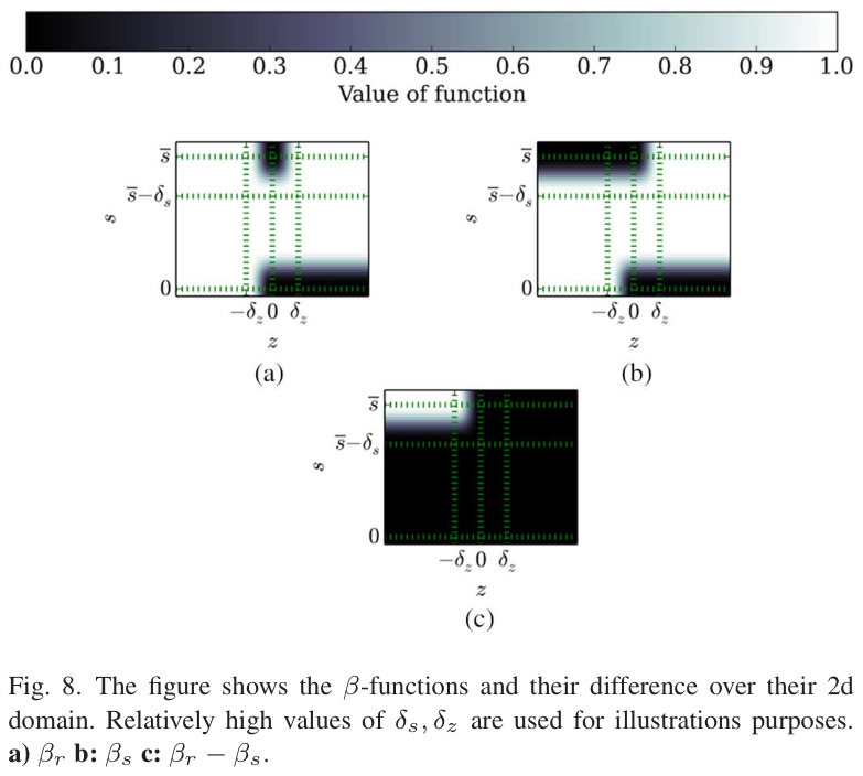
The appendix gives one construction satisfying the tank conditions. A fifth-order smooth step joins zero to one with vanishing first and second derivatives at both endpoints; its complement reverses that transition. These functions limit harvested damping energy near the tank cap and coordinate residual-energy transfer and control near depletion.
The experiments use a tank transition width equal to one tenth of the upper capacity and a residual-power transition width of 0.01. The exact coupling formulas and their plots are retained. Equations (27) and (28) also use an underlined lower-threshold symbol that the appendix does not explicitly define; no additional implementation value is inferred here.
Equations 25–28