At a glance
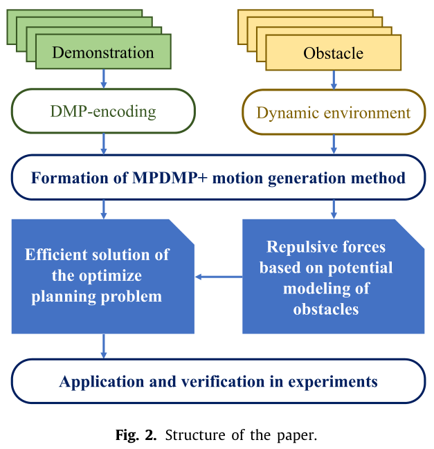
MPDMP+ generates new robot trajectories by combining several demonstrated movements with obstacle repulsion. Each demonstration is encoded as a DMP; MPC chooses its contribution over a short prediction horizon, and artificial potential fields supply separate avoidance forces. A proximal augmented Lagrangian method solves the resulting mixture-weight QP. Simulated paths and four Franka Emika setups illustrate the approach. The paper reports qualitative examples, without numerical runtime, error, or success-rate comparisons.
1. Introduction
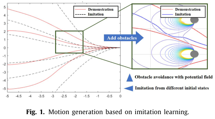
A movement primitive can reproduce a demonstrated path while adapting its start or goal. Learning from several demonstrations and avoiding moving obstacles requires additional structure. MPDMP uses predictive optimization to blend demonstrations during execution, so nearby reference trajectories can exert more influence. Earlier alternatives first fuse demonstrations and then plan around that combined reference. [11], [13], [21]
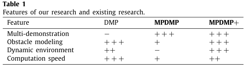
MPDMP+ separates two calculations: a constrained optimization chooses imitation weights, while obstacle potentials add repulsive forces. This avoids representing each obstacle as a nonlinear constraint in the mixture QP. The proximal solver is motivated by warm-startable optimization methods such as ProxQP. Table 1 is the authors’ qualitative feature comparison; its plus signs are not measured performance scores. [27], [36]
2. Problem formation
Human teaching supplies reference trajectories. The method fits a dynamical model to each demonstration, optimizes a combination of their forcing inputs, then adds independently computed obstacle forces. The formulation studied here is planar, with demonstrations directed toward a common stationary goal; extending it to three dimensions and several possible goals is future work.
2.1 Encoding demonstrations with DMP
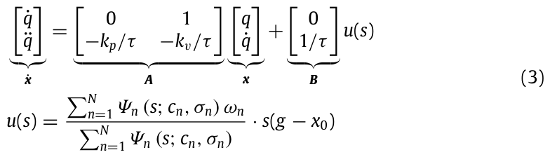
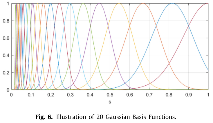
The DMP is a spring–damper system driven by a learned forcing term and a separate repulsive term. Translating the goal to the origin gives a linear state-space system in position and velocity, with nonlinear forcing controlled by a phase variable. Normalized Gaussian basis functions encode the forcing shape; their weights are learned through locally weighted regression. The displayed training objective fits acceleration residuals across demonstrations and can also optimize basis centers and widths. That joint fitting problem is nonlinear, unlike the subsequent mixture-weight QP. [37], [38]
The experiments use 20 basis functions. The stated canonical-system parameters are τ = 1 and αs = 0.1. Equation (4) describes exponential phase decay: it approaches zero asymptotically, although the surrounding source text says it reaches zero at t = τ. The original formulas are preserved for inspection.
Equations 1–6





2.2 Combining demonstrations
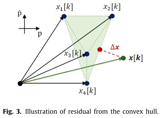
At each step the controller forms a weighted sum of the demonstrations’ forcing inputs. Weights are nonnegative and sum to one. The first loss measures the difference between the current state and a convex combination of reference states, using a symmetric positive-semidefinite weighting matrix. A small secondary term favors nearby demonstrations when several combinations give the same residual. These simplex constraints concern reference-state mixtures; they do not themselves constrain the executed robot to an obstacle-free region.
Equations 7–9





2.2 Prediction over a short horizon
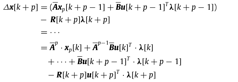
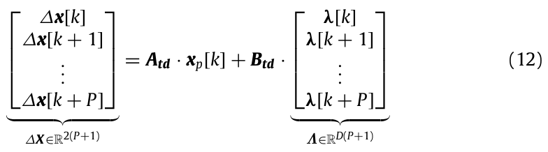
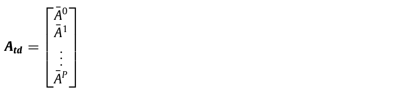
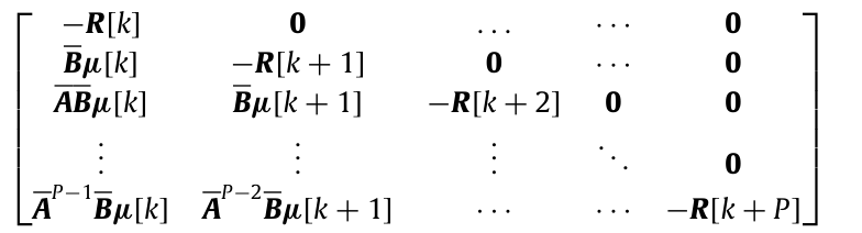
The continuous linear state model is discretized, then unrolled over the current step and a P-step future horizon. Stacking predicted residuals yields an affine function of the stacked demonstration weights. The optimization minimizes its weighted squared norm plus the proximity term, subject to one simplex constraint per step. The paper sets P = 3. Equations (10)–(13), the residual expansion, and both block matrices are retained.
Equations 10–13



3. Obstacle potentials
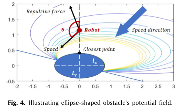
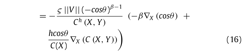
An elliptical obstacle is represented by its center, velocity, and axis lengths. Its potential grows with approach speed and proximity, and is switched off when the robot moves away. The repulsive term is the negative potential gradient. The chosen planar gains are h = 2, ς = 0.01, and β = 2. This construction builds on volumetric DMP obstacle potentials. [24], [27]
Equations 14–16 — first line



Equations 16 — continued–17

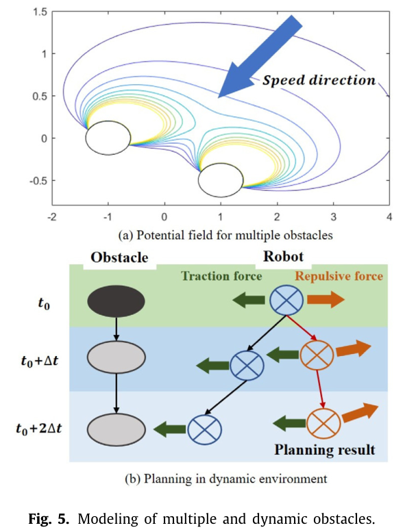
3. Multiple and moving obstacles
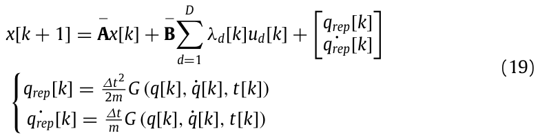
For several obstacles, the method assumes independent repulsive effects and sums their potential gradients. Moving obstacles are represented by a sequence of predicted future states aligned with the MPC horizon. During one state update, the repulsive force is held constant and converted to position and velocity offsets using a virtual mass. The paper discusses replacing the future-state sequence with a learned predictor, but its moving-obstacle experiment supplies the true trajectory. [39], [40]
Keeping avoidance outside the mixture QP simplifies that optimization. The paper does not establish a general collision-avoidance or closed-loop convergence guarantee for the combined dynamics with summed repulsive forces.
Equations 18–19

4. Optimization with a proximal method
The online planning problem becomes a linearly constrained QP in the stacked mixture weights. A proximal augmented Lagrangian solver updates primal weights and dual constraint multipliers. Its purpose is efficient repeated solution as the state changes; the paper does not report an independent solver benchmark.
4.1 Quadratic-program reformulation
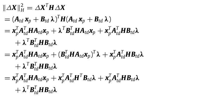
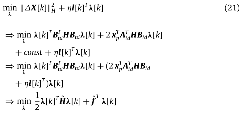
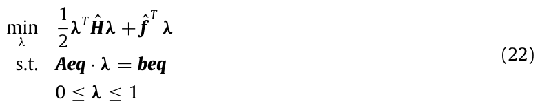
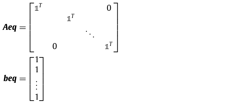
Expanding the residual loss removes terms that do not depend on the weights. The resulting Hessian is 2 BtdT H Btd, which is positive semidefinite when H is. Thus the runtime weight problem is convex. A block equality matrix enforces unit weight sums, and elementwise bounds keep weights between zero and one. This convexity statement concerns the mixture optimization, not learning basis locations or navigating the full obstacle field.
Equations Quadratic objective expansion–Equality-constraint matrix and vector


4.2 KKT and proximal updates
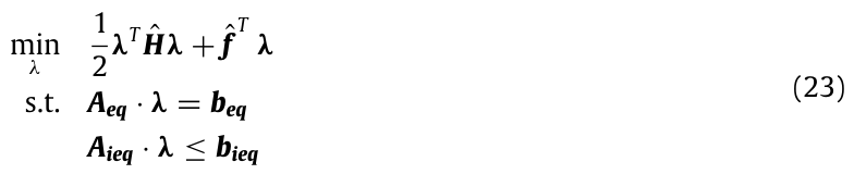
The solver starts from a QP with equality and inequality constraints and its Lagrangian. KKT stationarity, feasibility, and complementarity motivate a proximal saddle update. Positive regularization parameters stabilize the primal and dual subproblems, and inequality multipliers are projected onto the nonnegative orthant. Equation (25) does not explicitly print the usual nonnegativity condition on inequality multipliers; the update in Equation (27) imposes it. [36]
Equations 23–27



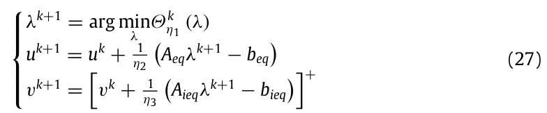
4.2 Augmented Lagrangians and stopping criterion
Eliminating dual updates gives a proximal augmented Lagrangian with quadratic equality penalties and a positive-part inequality penalty. A further primal–dual merit function supplies gradients and an optimality residual. The infinity norm of this residual sets the inexact inner stopping criterion. The retained derivation follows the cited proximal methods; printed notation and formulas are reproduced as published. [35], [41]
Equations 28–34
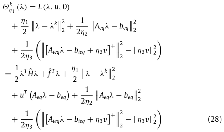

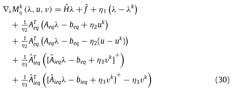




4.2 Newton step and line search
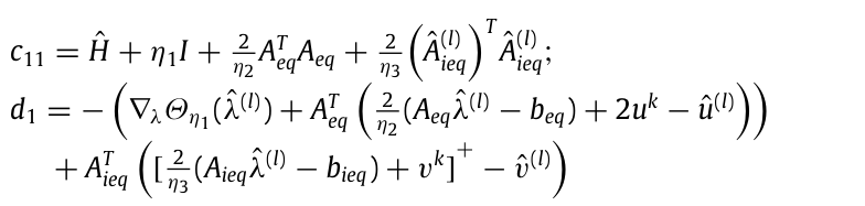
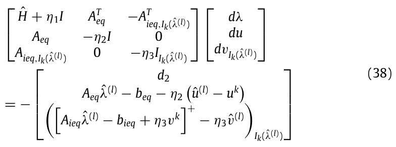
A semismooth Newton step solves a block system built from the current active inequality constraints. The positive-part map contributes only active rows to its generalized Jacobian. Eliminating intermediate terms produces a smaller system for the primal direction, equality multipliers, and active inequality multipliers; inactive multiplier directions are set separately. An exact line search on the primal–dual merit function selects the step length before updating all variables. Equations (35)–(40) and the intermediate coefficient definitions are retained.
Equations 35–40

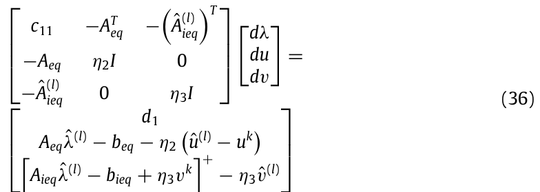




5. Experimental settings
The demonstration models use proportional gain Kp = 150 and damping Kv = 2√Kp ≈ 24.49. Evaluation consists of simulated trajectories and physical robot examples. There is no reported timing table, trial distribution, ablation, or quantitative comparison to the methods summarized in Table 1.
5.1 Simulation
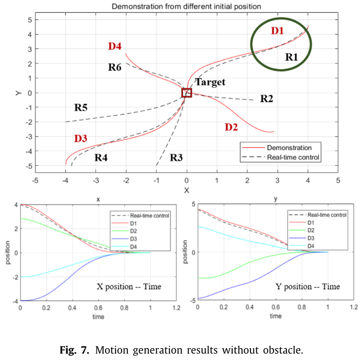
Four demonstrations start at different positions and reach (0, 0) with zero terminal speed. To prevent an initial detour toward the beginning of a reference trajectory, execution is initialized using its nearest demonstrated point. In obstacle-free examples, generated trajectories follow nearby demonstrations and reach the shared target; plotted position–time curves illustrate this resemblance.
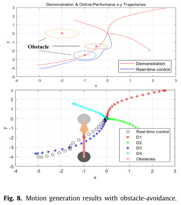
The avoidance examples contain three static obstacles or one moving obstacle. The moving-obstacle case changes the robot’s motion to yield to the obstacle. Its future trajectory is assumed known during planning, so the experiment does not measure robustness to prediction error. The claim that adding obstacles incurs little computational burden is qualitative here.
5.2 Robot experiments
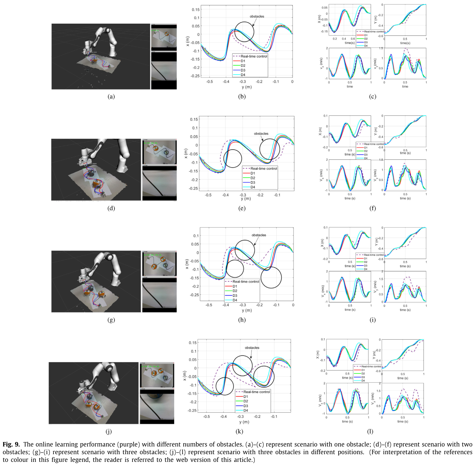
A Franka Emika arm is taught four trajectories for each of four obstacle arrangements. Camera detections approximate objects as ellipses or ellipsoids. The cases contain one obstacle, two obstacles, three obstacles, and three obstacles at different positions. Figure 9 shows the setup, generated paths, and position/velocity traces. The shown motions reach the goal while bending around obstacles and retaining aspects of the taught shape; the paper gives no aggregate success rate or physical moving-obstacle test.
6. Conclusion
The contribution is a combination of demonstration blending, short-horizon optimization, volumetric potential forces, and a proximal QP solver. The examples support its feasibility in the selected planar tasks. The authors propose extending the formulation to three-dimensional motion and multiple possible goals. Numerical solver comparisons, uncertainty in obstacle prediction, and broader empirical safety evidence are not supplied in this article.
Declarations and data availability
The authors declare no competing interests and state that they do not have permission to share the data. Funding includes the European Union’s Horizon 2020 Human Brain Project SGA3, the Hetao Shenzhen–Hong Kong cooperation-zone project, the Shanghai Rising Star Program, and the Tongji–Westwell joint laboratory.
Author information
The author information in the published article places Yingbai Hu, Wenjun Liu, Dianye Huang, and Alois Knoll at the Technical University of Munich; Mingyang Cui at Tsinghua University with a Munich affiliation; Jianghua Duan at the Hong Kong University of Science and Technology and its Shenzhen institute; and Guang Chen at Tongji University and Munich. Their stated research spans robot learning, control, intelligent vehicles, and perception. The original seven author portraits are retained below.