At a glance
Learned binary classifiers evaluate temporal task constraints directly on latent visual plans. Positive and negative image-sequence demonstrations train LSTMs; Boolean combinations of their outputs support more complex constraints. A simulated box-pushing study reports better classification than SVM and MLP baselines and accommodates human removal of boxes. These predictions are statistical and can accept invalid plans; the method does not provide formal verification guarantees.
1. Introduction
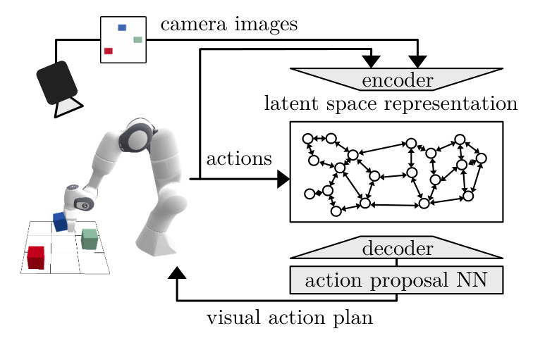
Visual-action planning learns a compact roadmap from image pairs and actions, avoiding a hand-built state model. Goal images specify desired configurations, but temporal requirements are difficult to impose on uninterpretable latent states. This work learns whether complete plans satisfy demonstrated requirements and filters candidate paths before action generation. [1]
1.2 Contributions
The contributions are latent-space constraint learning, empirical classifier evaluation, Boolean composition of learned constraints, and roadmap transitions after externally caused configuration changes.
2. Preliminaries
The approach combines a learned visual-action planner with finite-trace temporal logic.
2.1 Visual-action planning
A VAE with reconstruction and action losses groups nearby latent states into valid regions. The latent space roadmap connects regions when demonstrated actions link them. Graph search produces a latent plan, the decoder visualizes it, and the action proposal network predicts actions between consecutive states. Replanning can replace the initial state with the latest observation.
2.2 Linear temporal logic on finite traces
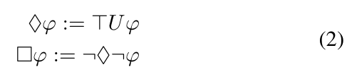
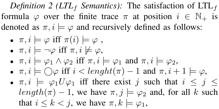
LTLf expresses Boolean and temporal requirements over finite sequences. Eventually requires a property before the trace ends; Always requires it through the end; Next requires a subsequent position. The original syntax, derived operators, and semantics are retained below. The source’s Until semantics contains a repeated-symbol typographical error; its explanatory clause uses the intended second formula. [16]
Equations 1–2

3. Constraints in visual planning
Given an image-derived execution and a temporal specification, the goal is to predict whether that execution satisfies the specification despite lacking an explicit symbolic model.
3.1 Learning constraints from demonstrations
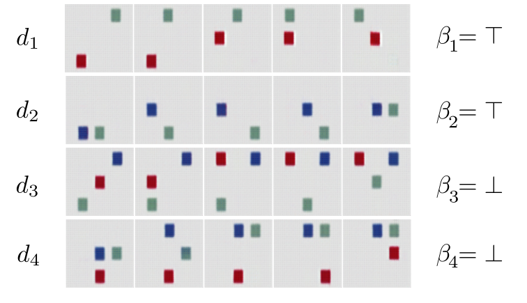
Humans label positive and negative image sequences for individual properties. The encoder maps each sequence to latent states while preserving its label, and an LSTM learns a binary decision from the sequence. Its recurrent memory is intended to capture temporal relations that flattened-image classifiers miss. [19]
3.2 Composition of constraints
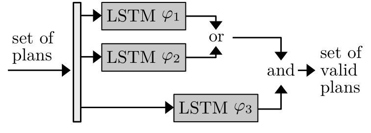
A Boolean expression tree combines independently trained classifiers. Each leaf evaluates a simple temporal property of the same plan, and internal conjunction, disjunction, or negation nodes combine those decisions. This reuses a library of learned properties, but classifier errors remain in the composed result.
3.3 Planning with task constraints
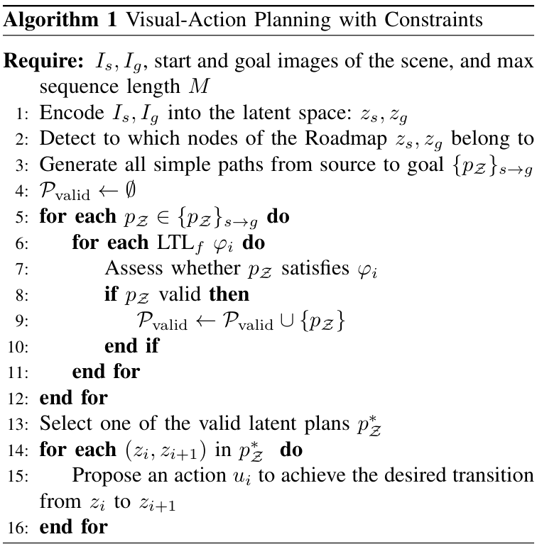
Encode start and goal images, locate their roadmap nodes, enumerate candidate simple paths, filter for the required constraints, and use the action network on a selected path. The prose requires satisfaction of all properties; the original pseudocode adds a path inside the per-property loop, an ambiguity worth resolving in an implementation. Exhaustive simple-path enumeration can also become costly on larger graphs.
4. Evaluation
PyBullet experiments model a warehouse-like box-pushing task. They compare classifier families, vary demonstration coverage and class balance, and test Boolean composition.
4.1 Task and visual-planning setup
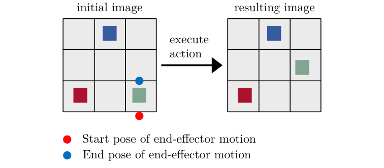
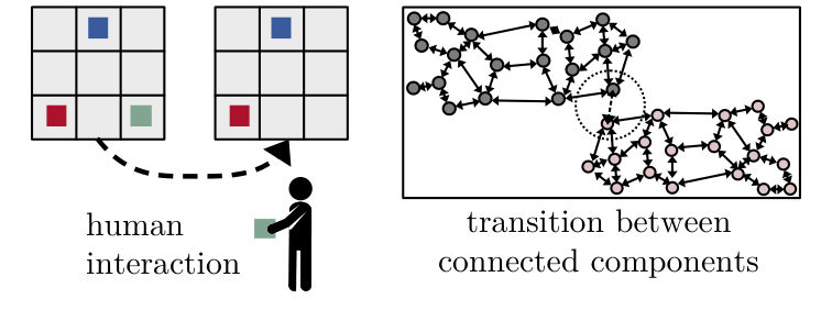
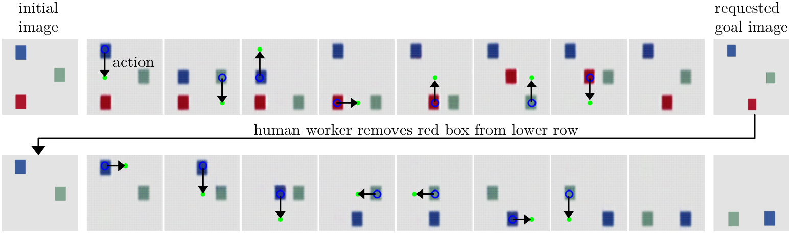
The simulated workspace is a 3×3 grid covering 0.45×0.45 m, with two or three boxes. Cardinal-direction pushes supply 5,000 image/action tuples, augmented by 2,000 contrastive pairs to separate configurations with different box counts. The learned roadmap has 831 nodes, six connected components, and 1,971 edges. Human box removal triggers re-encoding into a different component rather than a robot-executable edge.
4.2 Learning temporal constraints
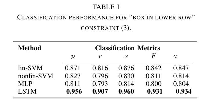
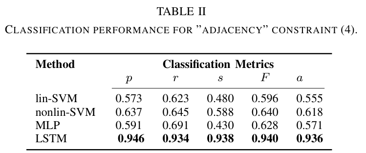
Two tests concern recurrent presence of a box in the lower row and restricted adjacency. The retained formulas define the exact finite-trace requirements; the adjacency formula forbids three consecutive states satisfying its adjacency observation. Synthetic labeled plans train separate four-layer LSTMs with 12 hidden features. Sequences are padded to eight 64-dimensional latent states. LSTM accuracy is 93.4% for the row constraint and 93.6% for adjacency, outperforming the reported SVM and MLP baselines. Precision is 95.6% and 94.6%, so invalid plans can still be accepted.
Equations 3–5



4.3 Demonstration size and balance
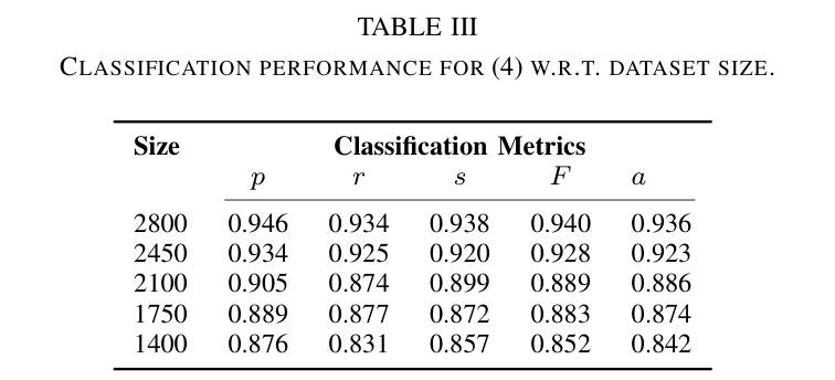
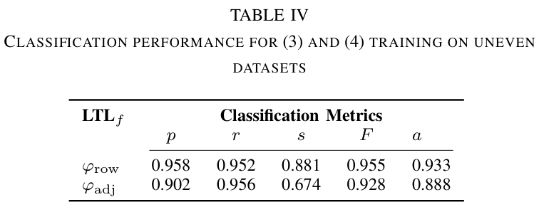
For adjacency, reducing training examples from 2,800 to 1,400 lowers accuracy from 93.6% to 84.2%. A 75%-positive dataset yields 88.8% accuracy but only 67.4% specificity for adjacency, showing that aggregate accuracy can hide a substantial false-positive problem. The authors recommend balanced examples.
4.4 Composing learned constraints
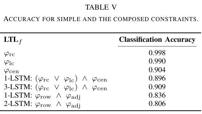
Three classifiers express eventual visits to either lower corner and avoidance of the center by the green box. Their Boolean composition reaches 90.9% accuracy versus 89.6% when learning that complete constraint directly. For the conjunction of row and adjacency constraints, composition scores 80.6% versus 83.6% directly. Thus reusable components can be competitive, but composition is not uniformly more accurate.

Equations 6–7


5. Conclusion
The study demonstrates reusable learned constraint filters in a small simulated visual-planning environment, including externally caused changes in box count. Reliability depends on labeled-data coverage, balanced examples, and classifier quality. The reported results support practical plan screening rather than guaranteed satisfaction on unseen executions.