At a glance
MDL treats learning as finding descriptions that compress observed data. This tutorial develops the connection from an informal two-part code to universal coding, normalized maximum likelihood and predictive model selection. It explains why model complexity is more than a parameter count, how Bayesian and sequential methods relate, and where approximation or model misspecification can make MDL perform poorly.
Chapter 1 Introducing the MDL Principle
1.1 Introduction and Overview
Model selection must balance fit against the ability to fit accidental noise. MDL measures that balance in bits: a useful regularity shortens the description of data after accounting for the model. The tutorial distinguishes this inference strategy from a belief that a simple model must be true.
1.2 The Fundamental Idea: Learning as Data Compression
Repeated patterns, biased frequencies and other regularities can all reduce description length, although they require different coding languages.
Regularity …
A repeated four-bit pattern is highly regular; a fair-coin string is usually incompressible; a string with four times as many zeros as ones has a weaker statistical regularity. These examples separate deterministic structure from distributional structure.
Equations 1.1–1.3
| (1.1) | |||
| (1.2) | |||
| (1.3) |
…and Compression
A loop compresses repetition; a literal print command usually cannot compress random data. A biased-coin code compresses skewed frequencies. Likewise, a short program can generate digits of π, a physical law can encode a table through coefficients and residuals, and grammar can compress language. Every saving depends on an agreed description method.
Equations
1.2.1 Kolmogorov Complexity and Ideal MDL
Kolmogorov complexity is the shortest program that prints the data and halts. Changing a universal language changes this length by at most a language-dependent constant, but that constant matters for small samples. The shortest-program problem is uncomputable, so ideal MDL is a conceptual foundation rather than a practical algorithm.
1.2.2 Practical MDL
Practical MDL restricts the description language so relevant code lengths can be computed. This sacrifices some detectable regularities but permits inference. Domain knowledge can guide the model class; no computable procedure can recover every possible regularity.
1.3 MDL and Model Selection
A high-degree polynomial can interpolate every training point while predicting poorly. Two-part MDL encodes both a hypothesis and the data conditional on it, selecting the smallest combined length. A point hypothesis is one distribution or function; a model is a family, such as all polynomials of one degree. The distinction matters when selecting parameters versus model structure.
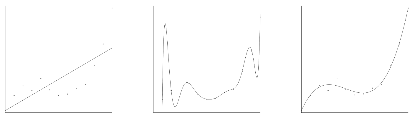
Crude4, Two-part Version of MDL Principle (Informally Stated) Let be a list of candidate models (e.g., is the set of -th degree polynomials), each containing a set of point hypotheses (e.g., individual polynomials). The best point hypothesis to explain the data is the one which minimizes the sum , where • is the length, in bits, of the description of the hypothesis; and • is the length, in bits, of the description of the data when encoded with the help of the hypothesis. The best model to explain is the smallest model containing the selected .
1.4 Crude and Refined MDL
The two-part objective becomes meaningful only after both coding rules are specified. Data codes have a principled probability interpretation; arbitrary hypothesis codes can distort inference.
Definition of L ( D | H )
For a probabilistic hypothesis, encode data with length equal to negative log likelihood. A regression function can be turned into such a distribution by specifying a noise model. The code then rewards high-probability observations.
Definition of L ( H ) : A Problem for Crude MDL
An arbitrary parameter code can make any chosen hypothesis cheap or expensive. Early minimax and discretization arguments constrain this freedom but can be cumbersome. Refined MDL replaces explicit parameter transmission with a universal code for the entire family.
Refined MDL
A universal code compresses nearly as well as the best family member chosen after observing the data. Refined MDL uses a minimax criterion to choose among such codes. The resulting one-part length is called stochastic complexity.
Parametric Complexity
Parametric complexity measures a family’s ability to fit possible datasets, including its geometry. Stochastic complexity decomposes into negative maximized log likelihood plus this complexity. Models with the same parameter count can therefore receive different penalties: the psychophysics example compares the greater flexibility of Stevens’ model with Fechner’s. The simplest NML formulation requires finite complexity and a restricted comparison setting.
Equation
1.5 The MDL Philosophy
Rissanen’s philosophy treats models as tools for discovering regularity, without requiring that a candidate distribution actually generated the observations.
1. Regularity as Compression
Learning separates compressible structure from residual information. Repetition is mostly structure; a fair-coin string mostly residual noise; biased frequencies supply structure while the precise order remains residual.
2. Models as Languages
A model is a language for expressing regularities. Noise is what remains expensive to encode relative to that language, rather than an intrinsic label on the data. Another model may expose structure previously treated as noise.
3. We Have Only the Data
Useful models can be known approximations: naive Bayes, speech models and linear economic models need not be literally true. MDL seeks an interpretation based on observed data and available models. This philosophical motivation does not itself guarantee robust behavior under misspecification.
4. MDL and Consistency
Consistency remains a sanity check: if a candidate distribution really does generate the data, the method should approach it with enough observations. Rates of convergence matter as well. MDL derives procedures from compression, then examines these statistical properties; exceptions and assumptions still require attention.
1.6 MDL and Occam’s Razor
Occam’s razor is an inference strategy: with limited evidence, a less flexible model can predict more reliably. The preferred complexity may grow as data accumulate.
‘1. Occam’s Razor (and MDL) is arbitrary’
Refined MDL constrains the code through minimax properties and can be invariant to parameterization. The claim that any encoding can arbitrarily determine its answer overlooks these restrictions; broader settings still require some modeling choices.
‘2. Occam’s Razor is false’
A complex underlying process can be best approximated by a simple model when samples are small. As evidence grows, richer polynomial families may improve the approximation. Minimizing training error over an unlimited family can overfit indefinitely. This is a justification for a fit–complexity trade-off, not a statement that nature is simple.
1.7 History
Rissanen developed MDL beginning in 1978, drawing on algorithmic complexity and information-theoretic model selection. Two-part codes evolved into predictive and mixture codes, then the connection to Shtarkov’s NML clarified parametric complexity. Wallace’s earlier MML shares coding ideas but uses a different Bayesian interpretation and optimization criterion.
1.8 Summary and Outlook
Practical MDL replaces an uncomputable shortest-program ideal with restricted, computable codes. Universal coding refines the crude model-plus-residual picture. The next chapter formalizes probability–length correspondence and the cost of selecting a model after seeing data.
Notes
“Crude MDL” is the tutorial’s pedagogical label, not a standard name for all early MDL work. Early theoretical papers already constrained coding schemes; some applications instead used ad hoc codes. The author also distinguishes Rissanen’s strong philosophical position from milder alternatives.
Chapter 2 Minimum Description Length Tutorial
2.1 Plan of the Tutorial
The technical route is prefix coding, statistical models, two-part MDL, universal codes, and four interpretations of refined MDL. Extensions address infinitely many models, undefined normalizers, regression and parameter estimation before discussing connections and failures.
2.2 Information Theory I: Probabilities and Codelengths
Two facts connect probability and coding: valid prefix lengths correspond to distributions through negative logarithms, and the code matching a generating distribution minimizes expected length.
Preliminaries and Notational Conventions - Codes
A code maps each datum to a distinct binary string so decoding is lossless. MDL compares code lengths, rather than needing to implement the actual bit strings. Logarithms are base two unless stated otherwise.
Preliminaries and Notational Conventions - Probability
A defective distribution assigns total mass below one. A probabilistic source has compatible distributions over successively longer sequences; an i.i.d. source factorizes into identical single-observation distributions.
2.2.1 Prefix Codes
No codeword in a prefix code begins another codeword, allowing concatenated messages to be decoded without separators. Every uniquely decodable code has an equivalent prefix code with the same lengths, so restricting attention to prefix lengths loses no relevant efficiency.
2.2.2 The Kraft Inequality - Codelengths and Probabilities, Part I
A fixed code can shorten only a small fraction of all strings: compressing a fair-coin sequence by many bits is exponentially unlikely. Designing a code after seeing the exact data is uninformative unless the code choice is itself charged.
Equations 2.1–2.3
| (2.1) | |||
| (2.2) | |||
| (2.3) |
A Most Important Observation
Kraft’s inequality links code lengths to probability masses. A uniform distribution gives fixed-length codes; nonuniform probabilities give shorter words to likelier outcomes. Ignoring a negligible rounding term permits ideal real-valued lengths. Prefix coding of arbitrary positive integers requires overhead beyond simply writing their binary value; the tutorial uses a simple approximately 2 log n code.
Probability Mass Functions correspond to Codelength Functions Let be a finite or countable set and let be a probability distribution on . Then there exists a prefix code for such that for all , . is called the code corresponding to . Similarly, let be a prefix code for . Then there exists a (possibly defective) probability distribution such that for all , . is called the probability distribution corresponding to . Moreover is a complete prefix code iff is proper (). Thus, large probability according to means small code length according to the code corresponding to and vice versa. We are typically concerned with cases where represents sequences of outcomes; that is, where is the sample space for one observation.
New Definition of Code Length Function
In MDL we are NEVER concerned with
actual encodings; we are only concerned with code length
functions. The set of all codelength functions for finite or countable
sample space
is defined as:
Equation
Equations 2.5
| (2.5) |
Continuous Sample Spaces
For continuous observations, densities correspond to code lengths at an agreed precision. Sums become integrals; comparisons must use a common precision so irrelevant discretization constants cancel.
2.2.3 The Information Inequality - Codelengths & Probabilities, II
If data follow P, coding with Q costs cross-entropy, minimized at Q=P. The information inequality formalizes the excess cost. With suitable independence or ergodicity assumptions, long-run average code lengths approach their expectations. A distribution can nevertheless be used as a code without claiming it is the true generator.
The that corresponds to minimizes expected
codelength
Let be a distribution on (finite, countable or continuous-valued)
and let be defined by
Equation
Equation
Summary and Outlook
Probability supplies both valid length assignments and an expected-efficiency criterion. The next step is to specify the candidate statistical models.
2.3 Statistical Preliminaries and Example Models
Markov chains provide a running example because model order controls flexibility while parameter estimates have a simple frequency interpretation.
Statistical Preliminaries
A parametric family is smoothly indexed by finitely many parameters. Maximum likelihood chooses the member assigning greatest probability to the observations. In binary Markov models, transition probabilities are empirical conditional frequencies; the number of parameters grows exponentially with order. Searching all orders using likelihood alone can memorize the sequence.
Equations 2.7–2.8
| (2.7) |
| (2.8) |
2.4 Crude MDL
Two-part MDL selects a hypothesis by adding its description length to negative log likelihood; model selection can then choose the smallest family containing that hypothesis.
2.4.1 Description Length of Data given Hypothesis
The conditional data length is negative log likelihood. This matches the optimal expected code when the hypothesis is correct and yields consistency in a finite family. Arbitrarily reassigning data codes to hypotheses can destroy even this elementary guarantee.
2.4.2 Description Length of Hypothesis
A hypothesis code must be fixed by a valid protocol. Uncharged dependence on sample size can reintroduce pure maximum-likelihood overfitting by making complex memorizing models artificially cheap.
Consistency of Two-part MDL
Fixed two-part codes give broad asymptotic consistency results, but finite-sample performance can remain poor. Encoding Markov order and empirical transition counts gives a concrete, initially crude parameter code.
Equations 2.9
| (2.9) |
Why (not) this code?
Encoding every possible empirical parameter value wastes precision. A coarser grid can reduce total length even if likelihood worsens slightly. The natural statistical resolution is often of order 1/√n rather than 1/n, motivating a principled regret criterion.
Equation 2.10
| (2.10) |
The Good News and the Bad News
Negative log likelihood is well motivated, but an arbitrary model code is not enough for good small-sample inference. Universal coding provides a broader framework in which coding choices can be compared and improved.
2.5 Information Theory II: Universal Codes and Models
A universal code competes with each code in a specified family. Two-part, Bayesian mixture and NML codes are different constructions with different guarantees.
Coding as Communication
Sender and receiver must agree on the decoding protocol before the message arrives. Choosing a convenient code after inspecting the data requires communicating that choice or integrating it into a shared universal code.
Universal Coding
Taking the shortest candidate length separately for every possible dataset generally fails Kraft’s inequality. A universal code must pay overhead to approximate that impossible hindsight oracle. The objective is small regret relative to the best candidate for each dataset.
Equations 2.11
| (2.11) |
2.5.1 Two-part Codes as simple Universal Codes
For a finite family, transmitting its best member’s index costs log of the family size, then the chosen code transmits the data. Countably infinite families need a nonuniform index code. Each fixed member can still be approached asymptotically, but there is no uniform constant overhead for all members.
Equations 2.12
| (2.12) |
2.5.2 From Universal Codes to Universal Models
A universal model is a single coding distribution representing a family; it need not belong to that family. A Bayesian mixture averages candidate distributions with fixed weights. For a discrete candidate with positive weight, mixture regret is bounded by the negative logarithm of that weight.
Equations 2.13–2.14
| (2.13) |
| (2.14) |
Bayes is Better than Two-part
For matching prior weights, a mixture code never uses more bits than selecting one weighted component and transmitting its index. This does not settle which prior or criterion is best; minimax regret supplies one answer.
Equations 2.15
| (2.15) |
2.5.3 NML as an Optimal Universal Model
Regret is extra code length relative to the best-fitting family member for the realized data. NML normalizes maximized likelihood across all possible datasets. If the normalizing sum/integral is finite, Shtarkov’s result makes it the unique distribution minimizing worst-case regret.
Equations 2.16–2.19
| (2.16) |
| (2.17) |
| (2.18) |
| (2.19) |
Proof
NML has the same regret for every dataset. Any different normalized distribution assigns less probability somewhere and therefore has larger worst-case regret. If the normalizer diverges, this construction is undefined and no finite constant-regret distribution exists.
Equations 2.20–2.21
| (2.20) |
| (2.21) |
Summary: Universal Codes and Models
Let be a family of
probabilistic sources. A universal
model in an individual sequence sense16 relative to , in this
text simply called a ‘universal model for ’, is a sequence
of distributions on respectively, such that for all ,
for all ,
Equation
2.6 Simple Refined MDL and its Four Interpretations
For finitely many models with finite complexity, choose the smallest NML code length: negative maximized likelihood plus the log normalizer. This stochastic complexity balances fit with a model’s ability to fit other possible data, rather than using training fit alone.
Equations 2.22
| (2.22) |
2.6.1 Compression Interpretation
NML shortens the description when the family fits better while imposing equal regret across datasets. This makes its coding criterion intrinsic to the model and sample space once those are specified.
Compression and Separating Structure from Noise
The fit term can be read as residual noise and the complexity term as the cost of distinguishable structure. This is relative to the chosen family, and the tutorial presents the interpretation more informally than the underlying minimax statement.
2.6.2 Counting Interpretation
Model complexity counts effectively distinguishable distributions. Nearly identical members do not contribute as much as clearly different ones. For a finite i.i.d. family, increasing data eventually distinguishes all members and complexity approaches log family size.
Equation 2.23
| (2.23) |
Asymptotic Expansion of P ¯ nml and COMP n
For regular k-dimensional families, complexity has a leading (k/2) log n term plus a Fisher-information volume term and a vanishing remainder. The geometric term matters for equal-dimensional or small-sample comparisons. The expansion requires regularity, interior estimates and suitable integrability; it can fail or converge slowly when dimension approaches sample size or the model is irregular.
Equations 2.24
| (2.24) |
Two-part codes and COMP n ( ℳ )
Optimally quantized two-part codes approach NML regret up to a bounded dimension-dependent overhead under regularity assumptions. This does not justify arbitrary parameter discretizations used in some applications.
Equation
2.6.3 Bayesian Interpretation
Bayes-factor selection compares marginal likelihoods. Its relation to MDL depends on the prior, family regularity and whether the data-generating process belongs to the family.
Equation 2.25
| (2.25) |
ℳ is Exponential Family
For regular exponential families, a Laplace approximation relates mixture-code regret to Fisher information and the prior density. Jeffreys’ prior cancels the parameter-dependent part, giving asymptotically minimax regret and agreement with NML under the stated conditions.
Equations 2.26–2.27
| (2.26) |
| (2.27) |
ℳ is not an Exponential Family
Outside exponential families, observed rather than expected Fisher information enters the approximation. With correct specification they converge under regularity conditions; under misspecification an order-one discrepancy can remain. Bayes and NML are therefore not universally identical.
Equation 2.28
| (2.28) |
2.6.4 Prequential Interpretation
Distributions as Prediction Strategies
The chain rule expresses a joint distribution as successive predictive distributions. Negative joint log likelihood equals cumulative one-step log loss. This gives every sequence code a predictive interpretation: predict the next outcome using only the preceding outcomes.
Equations 2.29–2.30
| (2.29) |
| (2.30) |
Log Loss for Universal Models
Predictive MDL evaluates a sequence of estimators on data they have not yet seen. Plug-in maximum likelihood can be near-optimal under conditions but can also assign zero probability disastrously: a first observed zero makes a later one impossible in naive Bernoulli estimation. Laplace or Jeffreys smoothing avoids that failure; Jeffreys’ half-count rule approaches NML for the Bernoulli model.
Equations 2.31–2.34
| (2.31) |
| (2.32) |
| (2.33) |
| (2.34) |
Summary
Compression, distinguishable-model counting, Bayesian mixture behavior and sequential log loss explain the same refined selection criterion under their respective assumptions.
2.7 General Refined MDL: Gluing it All Together
Two complications require extensions: infinitely many candidate families and models with divergent NML normalizers. Both can be addressed by constructing an additional valid universal code.
2.7.1 Model Selection with Infinitely Many Models
Comparing infinitely many family code lengths without charging a family index can recreate memorization. Add a prefix length for the model index, often a slowly growing integer code. For a finite family this index charge can be uniform and cancel in comparisons.
Equation 2.35
| (2.35) |
2.7.2 The Infinity Problem
Even the unrestricted Gaussian location family has infinite NML complexity. Restricting the range makes a conditional normalizer finite, but the restriction must be encoded or otherwise chosen through a valid protocol. A meta-code communicates the needed range with small overhead relative to hindsight, rather than selecting an arbitrary cutoff for free.
Equations 2.36–2.38
| (2.36) |
| (2.37) |
| (2.38) |
Renormalized Maximum Likelihood
Renormalized maximum likelihood attempts a more efficient one-part solution by normalizing a likelihood already optimized over a range parameter. It improves on duplicated descriptions in a meta two-part code, but its applicability still requires checking the resulting normalizer.
Equation 2.39
| (2.39) |
Region Indifference
Generalized schemes can prefer particular parameter regions. Changing an origin may change some code lengths. Conditioning an improper Jeffreys prior on initial observations offers another approach, though its integration into the tutorial’s MDL framework is not settled.
2.7.3 The General Picture
The common principle is to construct one valid code that competes as evenly as possible with the available candidate descriptions. Infinite settings force some nonuniform preference. When computation only finds local likelihood maxima, complexity should reflect that actual estimator’s ability to fit data rather than the unattainable global optimum.
GENERAL ‘REFINED’ MDL PRINCIPLE for Model Selection Suppose we plan to select between models for data . MDL tells us to design a universal code for , in which the index of is encoded explicitly. The resulting code has two parts, the two sub-codes being defined such that 1. All models are treated on the same footing, as far as possible: we assign a uniform prior to these models, or, if that is not a possible, a prior ‘close to’ uniform. 2. All distributions within each are treated on the same footing, as far as possible: we use the minimax regret universal model . If this model is undefined or too hard to compute, we instead use a different universal model that achieves regret ‘close to’ the minimax regret for each submodel of in the sense of (2.38). In the end, we encode data using a hybrid two-part/one-part universal model, explicitly encoding the models we want to select between and implicitly encoding any distributions contained in those models.
Equations 2.40
| (2.40) |
Summary
Refined MDL combines minimax universal codes with additional valid coding layers when a single finite normalizer is unavailable. The model-selection prescription then needs further adaptation for other inference tasks.
2.8 Beyond Parametric Model Selection
MDL extends to density estimation, parameter estimation, regression and classification. Extensions do not inherit every model-selection guarantee automatically.
Non-Parametric Inference
Nonparametric estimation can compare increasingly rich model classes that approximate an infinite-dimensional target. Complexity controls how quickly flexibility grows with available evidence.
MDL Parameter Estimation: Three Approaches
After selecting a family, one may use its maximum-likelihood estimate, an optimally quantized two-part estimate, or a predictive estimate. They can agree asymptotically in fixed-dimensional regular families while differing substantially on small samples.
Regression
With Gaussian residuals, conditional negative log likelihood is proportional to squared error plus noise-scale terms. Compare conditional universal codes for outputs given inputs and charge the model index. Input lengths can be ignored only when their coding rule is identical across candidates.
Equations 2.41–2.44
| (2.41) |
| (2.42) |
| (2.43) |
| (2.44) |
When the Codelength for Can Be Ignored If all models under consideration represent conditional densities or probability mass functions , then the codelength for can be ignored in model and parameter selection. Examples are applications of MDL in classification and regression.
‘Non-probabilistic’ Regression and Classification
Direct loss-based regression and classification aim to avoid explicit noise assumptions, but some MDL classifications can overfit persistently under misspecification. Proposed fixes need not retain a natural literal coding interpretation. The tutorial treats this as an unresolved limitation, not a universal robustness guarantee.
Summary
The general coding viewpoint is broader than one formula. Whether an extension predicts well must be checked for its model class, loss and approximation.
2.9 Relations to Other Approaches to Inductive Inference
MDL is related to Bayesian inference, MML, prequential validation, cross-validation and algorithmic complexity. Similar-looking criteria can have distinct objectives and assumptions.
2.9.1 What is ‘MDL’?
Here MDL means inductive inference using universal models, while refined MDL refers more specifically to the minimax model-selection construction. It is neither restricted to a BIC formula nor a label for every conceivable compression heuristic.
2.9.2 MDL and Bayesian Inference
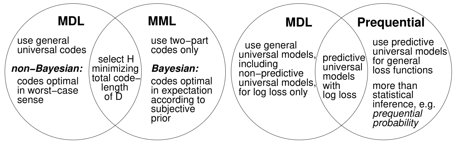
NML, predictive codes and estimator-dependent variants are not generally Bayesian mixtures. Bayesian methods remain important implementations within the broader MDL viewpoint.
MDL as a Maximum Probability Principle
MDL interprets distributions primarily as predictive/coding devices and need not update every construction through a prior and posterior. When it uses a prior, coding regret guides its choice. This offers an interpretation for useful but known-imperfect models, while the tutorial acknowledges Bayesian philosophies that also accommodate such use.
MDL and BIC
BIC keeps negative maximized log likelihood plus (k/2) log n and drops order-one terms. That is a fixed-dimensional asymptotic approximation, not the full MDL principle. It can lose important geometric effects and behave differently when the candidate dimension grows with sample size.
Equation 2.45
| (2.45) |
MDL and MML
MML chooses a two-part description minimizing expected absolute length under a subjective prior; refined MDL emphasizes worst-case relative length. MML naturally selects both family and parameters and can provide an invariant, interpretable point summary when a full posterior mixture is unwieldy.
2.9.3 MDL, Prequential Analysis and Cross-Validation
Prequential validation scores forecasts made before each observation. Log-loss versions correspond to code lengths, while Dawid’s framework also permits other losses. Compared with ordinary cross-validation, the sequential protocol never uses future data to predict past data and predicts each outcome once.
2.9.4 Kolmogorov Complexity and Structure Function; Ideal MDL
Ideal MDL uses universal programs to describe computable distributions, but cannot generally find the optimizing description. Kolmogorov’s structure-function viewpoint instead isolates a model capturing all compressible structure, leaving typical residual noise. Sending only that structure suggests lossy compression and links practical MDL to the theoretical separation of structure and randomness.
Equation 2.46
| (2.46) |
Summary and Outlook
These connections supply useful interpretations without making the methods identical. Their practical performance depends on the detailed procedure.
2.10 Problems for MDL?
Conceptual objections about simplicity must be separated from concrete failures caused by approximation, computational constraints or misspecified models.
2.10.1 Conceptual Problems: Occam’s Razor
The relevant question is whether a coding prescription is justified and predicts well, not whether the world is intrinsically simple.
1. ‘Occam’s Razor (and MDL) is arbitrary’ (page 1.6 )
Finite, well-defined NML comparisons are invariant to smooth reparameterization. Infinite families, divergent normalizers and the choice of submodel hierarchy introduce unavoidable preferences. Such choices should be explicit rather than disguised as universally intrinsic simplicity.
2. ‘Occam’s razor is false’ (page 1.6 )
A complexity penalty can yield consistency where unrestricted maximum likelihood overfits. That supports the strategy of starting simple at small samples, but does not prove MDL optimal for every loss, setting or finite dataset.
2.10.2 Practical Problems with MDL
Poor results can follow from using asymptotic expansions too early or cutting off parameter ranges arbitrarily. Prefer the actual NML or an appropriate mixture when defined and computable; otherwise use a carefully designed predictive or two-part code. The validity of approximations remains a practical research question.
MDL and Misspecification
A deeper problem arises when no candidate distribution approximates the data well: MDL and Bayes can choose poor predictive approximations, including persistent classification overfitting. This matters precisely because MDL’s philosophical motivation sought to avoid reliance on a true model.
2.11 Conclusion
Universal coding unifies several sensible inference strategies and often gives strong consistency and convergence results. It remains fallible under some practical approximations and misspecification. Further refinement is needed; compression alone is not a blanket guarantee of predictive success.
Further Reading
The bibliography includes the foundational Rissanen work and surveys by Barron, Rissanen, Yu and others. Earlier monographs remain useful for the philosophy even where their technical prescriptions have been superseded.
Acknowledgments
The author thanks Jay Myung, Mark Pitt, Steven de Rooij and Teemu Roos for comments on the tutorial.
Notes
The notes qualify technical conventions: code lengths can be idealized, finite-sample codes must charge any data-dependent choice, and individual-sequence universality differs from expected universality. Not every universal distribution forms a compatible probabilistic source across sample sizes. Claims about consistency, Bayesian equivalence and empirical success depend on the cited conditions.