At a glance
A neural network can be regularized by charging for the information in its weights. Hinton and van Camp learn independent Gaussian weight distributions and minimize expected prediction error plus a description-length penalty. Bits-back coding makes that penalty a KL divergence. Exact moment propagation is available for one nonlinear hidden layer with linear outputs. The small empirical study is promising but explicitly preliminary, and a lower-cost trivial solution exposes a weakness of the tested objective.
1 Introduction
With scarce training data, many adjustable weights can memorize outputs. Restricting connections, sharing weights or quantizing values reduces capacity, but each controls information only indirectly or complicates optimization. The paper instead learns how precisely each weight must be specified.
2 Applying the Minimum Description Length principle
A sender transmits a network’s weights and the residuals needed to reconstruct every training output. MDL trades the length of these two messages: added model complexity is worthwhile only when it reduces residual coding cost. The architecture is assumed agreed in advance [7].
3 Coding the data misfits
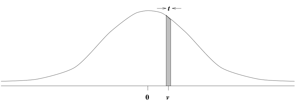
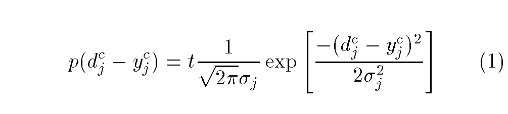
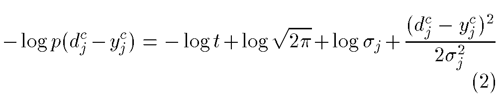
Assume finely quantized, Gaussian residuals for each output. Negative log probability yields a squared-error term. Optimizing residual variance gives a log mean-squared-error cost plus constants. The cost of transmitting the fitted variance is acknowledged but ignored in the implementation.
Equations 1–3

4 A simple method of coding the weights
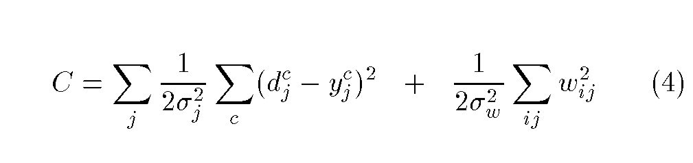
A fixed zero-mean Gaussian weight code gives the familiar squared-weight penalty. An adaptive Gaussian mixture can exploit weight clusters [6], but fixed precision still wastes bits on weights whose exact values barely affect predictions. The next construction learns this precision during training.
Equation 4
5 Noisy weights
Replace one weight vector by a factorized Gaussian distribution, learning a mean and variance for every weight. More variance makes a weight cheaper to communicate but raises expected prediction error. The objective jointly balances these effects.
5.1 Expected description length of the weights
Given an agreed Gaussian coding prior P and a learned Gaussian posterior Q, the effective cost of communicating a weight is KL(Q‖P). The direction is fixed by averaging under the learned distribution Q.
Equation 5

5.2 The bits-back argument
Sample a precise weight from Q using random bits, encode it under P, then transmit the resulting output residuals. Once the receiver reconstructs the training outputs, the shared learning procedure recovers Q and the random bits used to select the sample. Subtracting those recovered bits leaves the KL cost rather than the full precision cost.
Equations 6–9




5.3 Expected description length of the data misfits
Independent Gaussian weights make each hidden preactivation Gaussian. A precomputed table maps its mean and variance through the nonlinearity. Independence across hidden units and linear output units then allow exact output moments and expected squared error. A second derivative table supports backpropagation through these moments. This exact argument applies to the stated one-hidden-layer architecture, not arbitrary deep networks.
Equations 10–14





6 Letting the data determine the prior
The coding prior’s mean and variance are learned jointly with the weight distributions. A complete Bayesian treatment could charge for transmitting these parameters using hyperpriors; the experiments ignore that cost. This makes the coding prior data-dependent and limits a literal full-description interpretation.
6.1 A more flexible prior distribution
An adaptive Gaussian mixture encodes clusters of weights more economically than one broad Gaussian. The exact KL from a Gaussian posterior to a mixture has an intractable log-sum expectation. A tractable upper bound uses componentwise Gaussian KL values inside a weighted log-sum-exp. The mixture parameters’ own coding cost is again omitted.
Equations 15–17



7 Coding with a Gaussian mixture
The four-step protocol below transmits a component choice and sampled weight, then recovers both sources of randomness. Choosing component probabilities exponentially in their KL costs produces the tractable upper bound. The steps and equations are retained in full.
Mixture coding procedure
- Randomly pick one of the Gaussians in the mixture with probability rᵢ given by Equation 18.
- Communicate the choice of Gaussian to the receiver. If we use the mixing proportions as a prior for communicating the choice, the expected code cost is Equation 19.
- Communicate the sample value to the receiver using the chosen Gaussian. Taking into account the random bits recovered when the receiver reconstructs the posterior, the expected sample cost is Equation 20. The combined component-choice and sample cost is Equation 21.
- After receiving samples from all posterior weight distributions and the training errors, the receiver runs the learning algorithm to reconstruct those posteriors and all component divergences. This recovers the random bits used to choose a Gaussian. The bits-back quantity to subtract is the component-choice entropy in Equation 22.
Equations 18–22





7.1 A statistical-mechanics lemma
At unit temperature, expected energy minus entropy is minimized by Boltzmann probabilities. Identifying each mixture component’s effective energy with its KL cost minus log mixture weight turns the optimized free energy into the negative log partition sum used in the bound.
Equations 23–25



8 Implementation
Finite-difference checks compare each predicted gradient with the actual change in the objective. A 300×300 lookup table with linear interpolation gave reasonably accurate derivatives in this implementation. The check tests derivatives; it does not establish that the objective has a useful global optimum.
9 Preliminary results
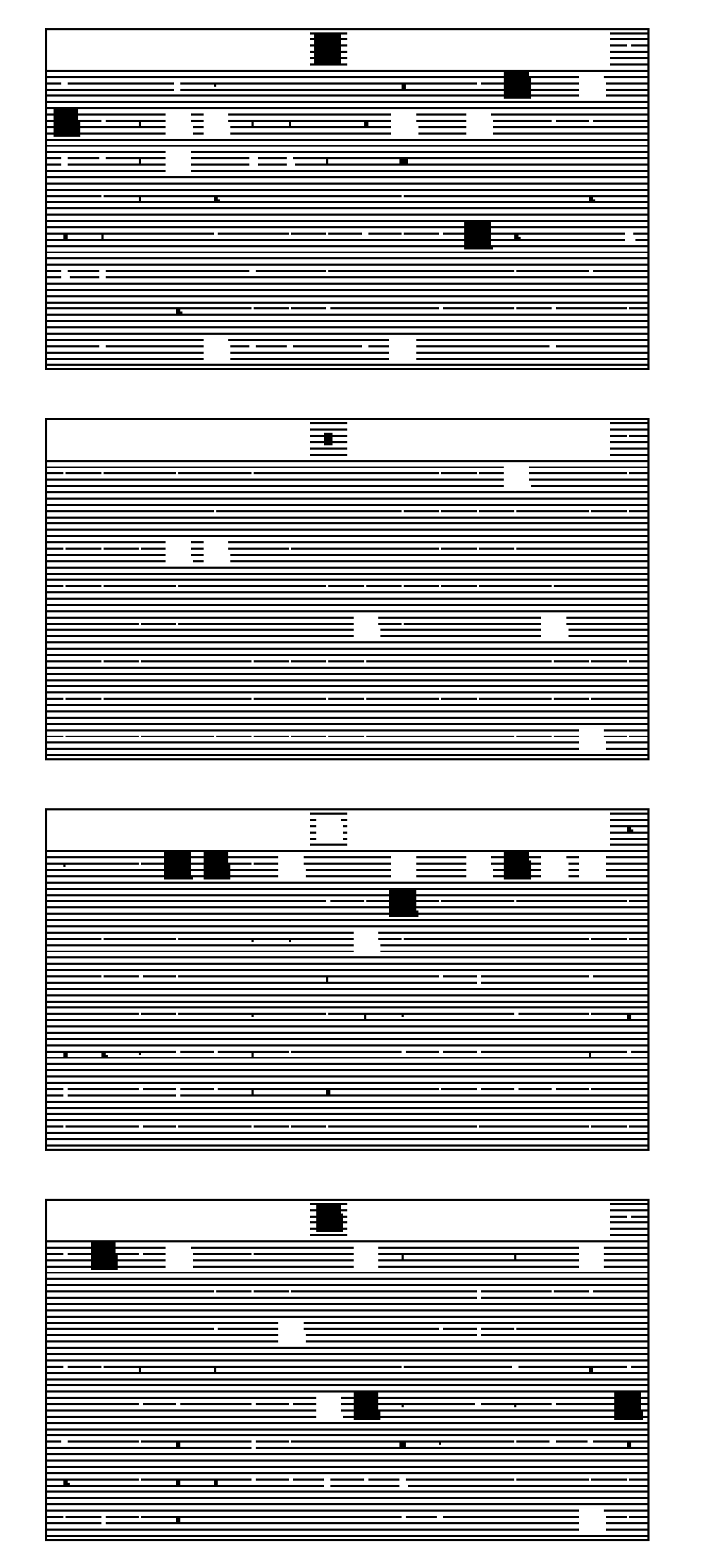
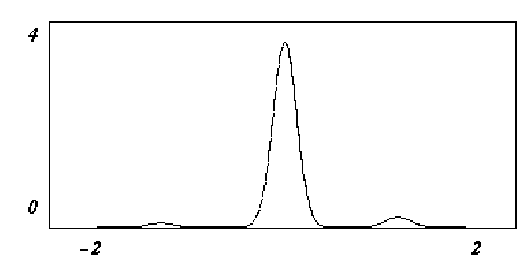
One peptide-effectiveness task uses 128 inputs, four hidden units and 521 weights, trained on 105 examples and tested on 420. Five Gaussian prior components and all weight distributions are optimized jointly. Starting the weight penalty at full strength collapses predictions to the mean, so the authors gradually raise its coefficient from 0.05 to 1. Across five starts, the selected useful solution has relative test squared error 0.286, versus 0.967 without information regularization and 0.317 for validation-tuned weight decay. Test-tuned 0.291 comparisons are explicitly acknowledged as invalid model selection.
The evidence is a single small task, not a broad benchmark. More seriously, the constant predictor still attains a lower total description length than the useful solution and has relative error near one. The paper calls this a failure of the MDL principle or of the chosen coding scheme; it must not be hidden by the favorable result.
Equations 26–27


10 Discussion
Exact Bayesian prediction averages over the full posterior but is generally intractable. Monte Carlo [5] preserves complex posterior shape; Laplace methods [4] approximate a local optimum. This method instead optimizes a diagonal Gaussian throughout learning. Ignoring weight correlations may matter, and suppression of those correlations is only a proposed mechanism. Weight noise also smooths activation probabilities, potentially permitting threshold hidden units.
11 Acknowledgments
The work acknowledges NSERC support and discussions with David MacKay, Radford Neal, Chris Williams and Richard Zemel. Hinton was a fellow of the Canadian Institute for Advanced Research.