At a glance
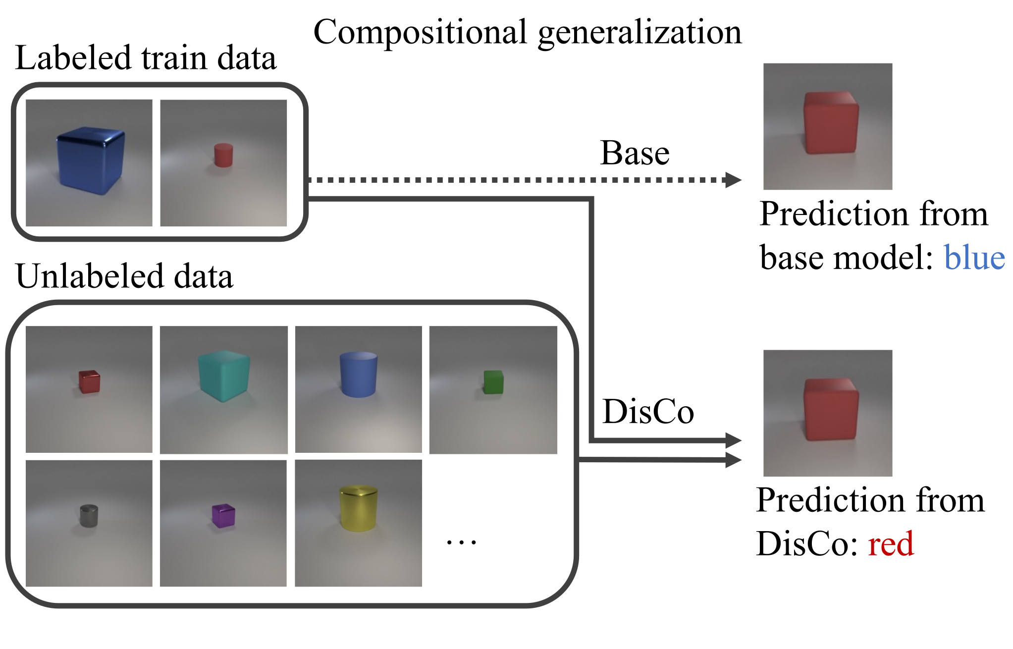
DisCo improves compositional visual question answering (VQA) by adapting a pretrained model to unlabeled images containing new or rare attribute combinations. It pairs these images with training questions, accepts low-entropy answer predictions as pseudo-labels, and trains on accepted examples together with labeled examples.
A confidence-based distribution-coverage score selects model checkpoints without target answer labels. Experiments use synthetic CLEVR datasets and three VQA backbones. The main setting exposes target-distribution images during adaptation and selection; a separate evaluation tests genuinely unseen images from that distribution.
1. Introduction
A model trained mostly on blue cubes and red cylinders may fail on red cubes even though it has learned the individual colors and shapes. DisCo uses unlabeled images of such combinations to extend a model’s learned associations.
The approach does not require additional human answers for those images, but does require suitable unlabeled visual data and a base model with enough correct, confident predictions to start self-training.
3. Method
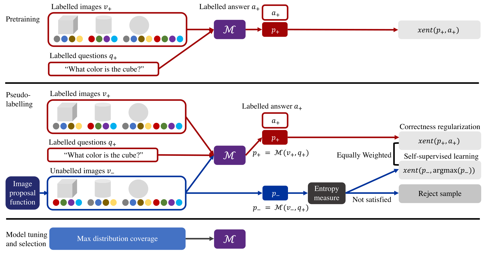
The framework has three stages: train a base VQA model, iteratively add confident image/question/answer pseudo-labels from an unlabeled pool, and choose a checkpoint using the fraction of candidate pairs accepted by the confidence rule.
3.1. Problem formulation
Labeled examples are image/question/answer triplets from a biased color–shape distribution. The unlabeled pool primarily supplies a different distribution of combinations. The target is object-level compositional generalization: recognizing familiar attributes when they occur in different combinations.
The experiments distinguish no labeled examples of the reversed combinations from settings with small proportions of those combinations. Thus some reported gains address rare combinations rather than entirely unseen labeled combinations.
3.2. Iterative pseudo-labeling
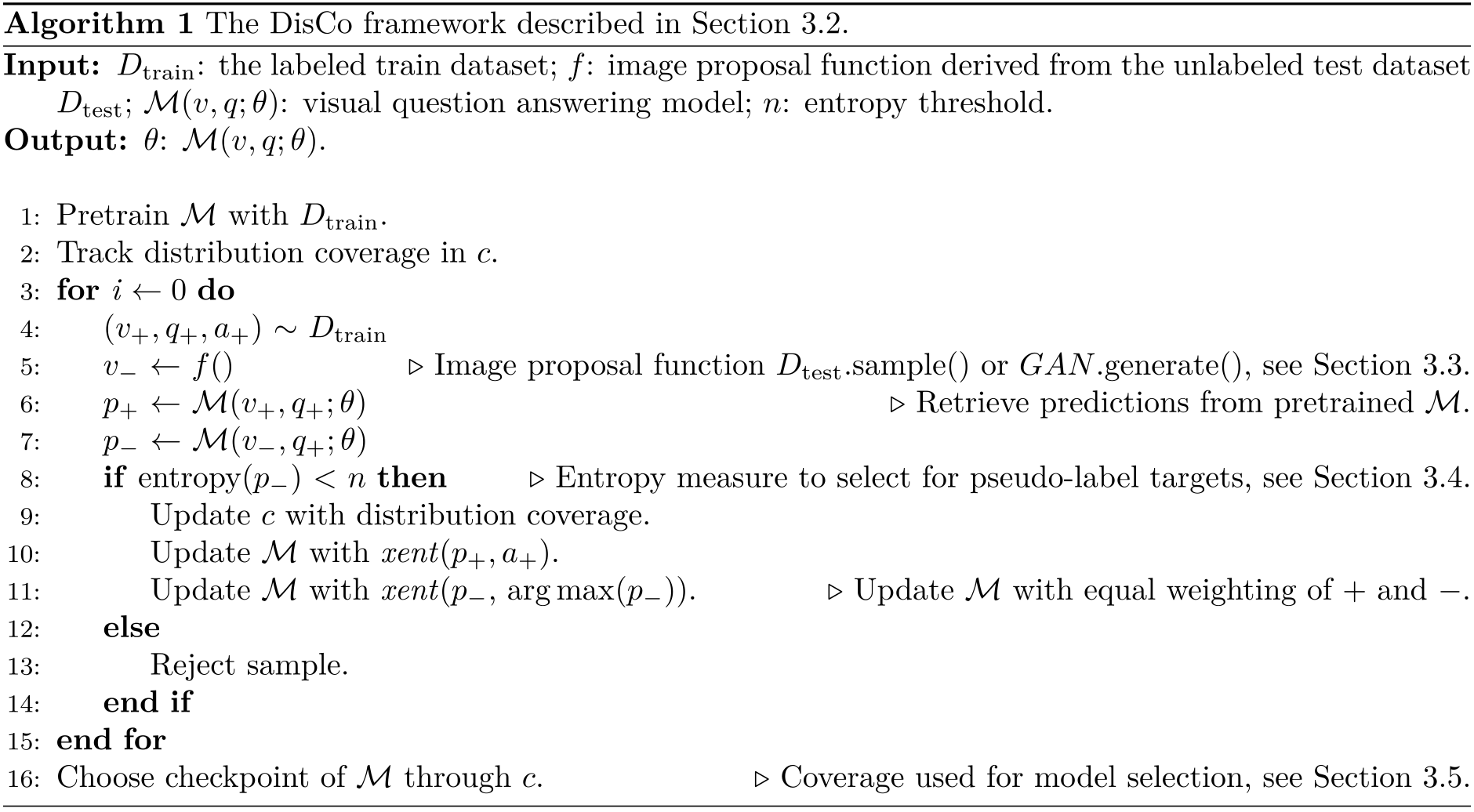
Algorithm 1 and Figure 2 preserve the complete procedure. A question sampled from labeled training data is paired with an unlabeled proposed image. The current model supplies an answer distribution; if its entropy is below the threshold, its highest-probability answer becomes a pseudo-label.
An accepted pseudo-labeled example and a labeled example receive equally weighted cross-entropy training. The labeled term is intended to anchor correctness while learning from the new distribution. Rejected candidate pairs do not supply pseudo-label updates. The original sixteen-step algorithm is retained without altering its printed loop notation.
3.3. Image proposals
DisCo-S directly samples unlabeled target images. DisCo-G trains an unconditional StyleGAN2 on the same unlabeled pool and uses generated images as proposals [14]. The generator can vary scenes beyond the finite pool but introduces its own image-quality and coverage limitations.
Both routes use information from the unlabeled distribution. Generated proposals do not make the method independent of access to target-like images.
3.4. Entropy filtering
Random pairing creates two error sources: the question’s referred object may not exist, or the model may answer incorrectly despite a valid referent. Entropy, H(p) = −∑ pᵢ log pᵢ, is used as an empirical filter for both.
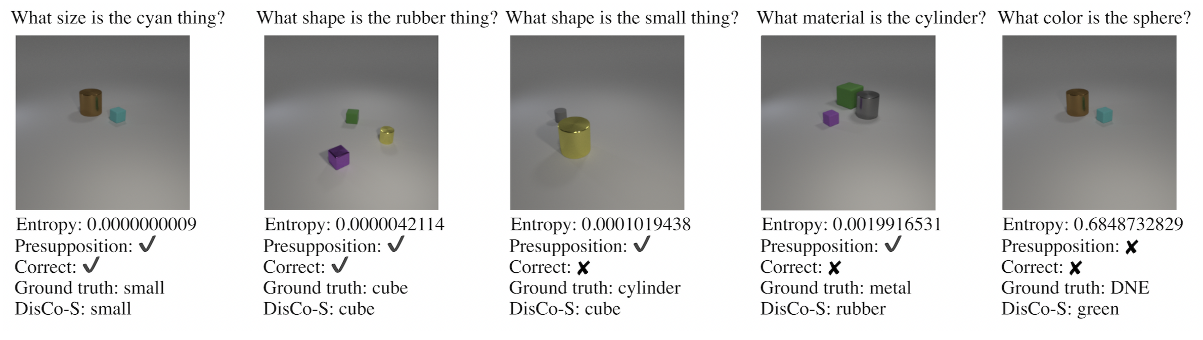
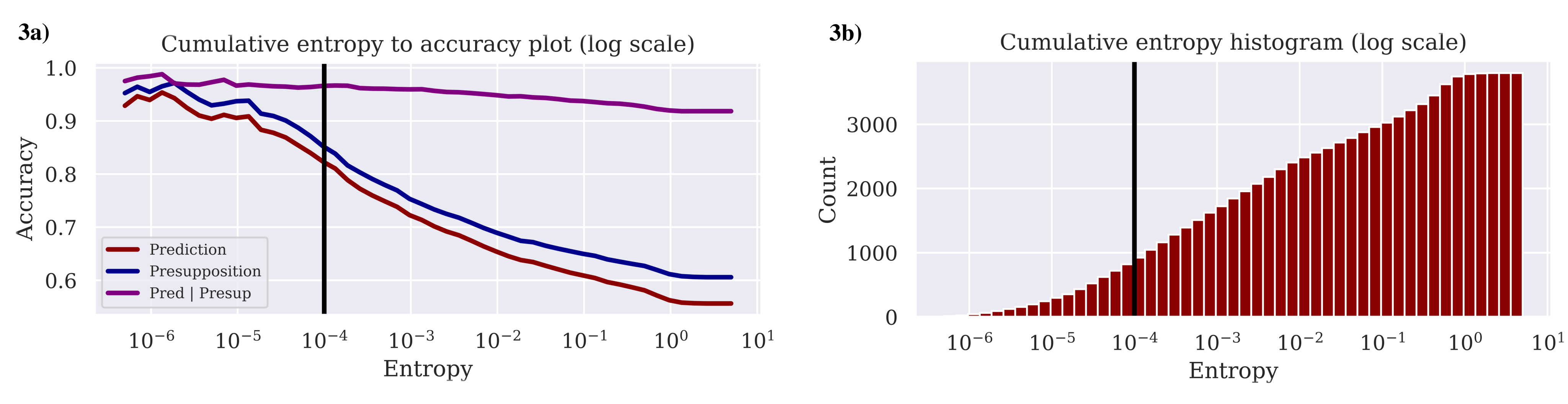
At the illustrated threshold near the thirtieth percentile, 85.06% of accepted pairs satisfy the question’s presupposition, and 82.07% both satisfy it and have the correct answer. Conditional accuracy among valid pairs is 96.48%. These are different denominators; low entropy does not eliminate erroneous pseudo-labels.
Figure 3 shows the largest change in presupposition adherence as the entropy threshold expands, while accuracy conditional on adherence changes less. This supports the filter’s usefulness in this dataset without establishing universal confidence calibration.
3.5. Model selection
Coverage is the fraction of proposed image/question pairs that pass entropy filtering. The checkpoint with greatest coverage is selected. This is confidence coverage under the sampling and threshold rule, not a direct measurement of all distinct semantic combinations covered.
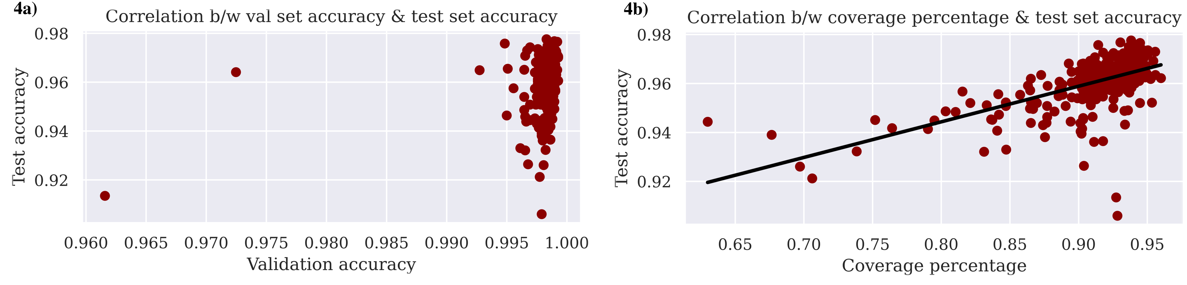
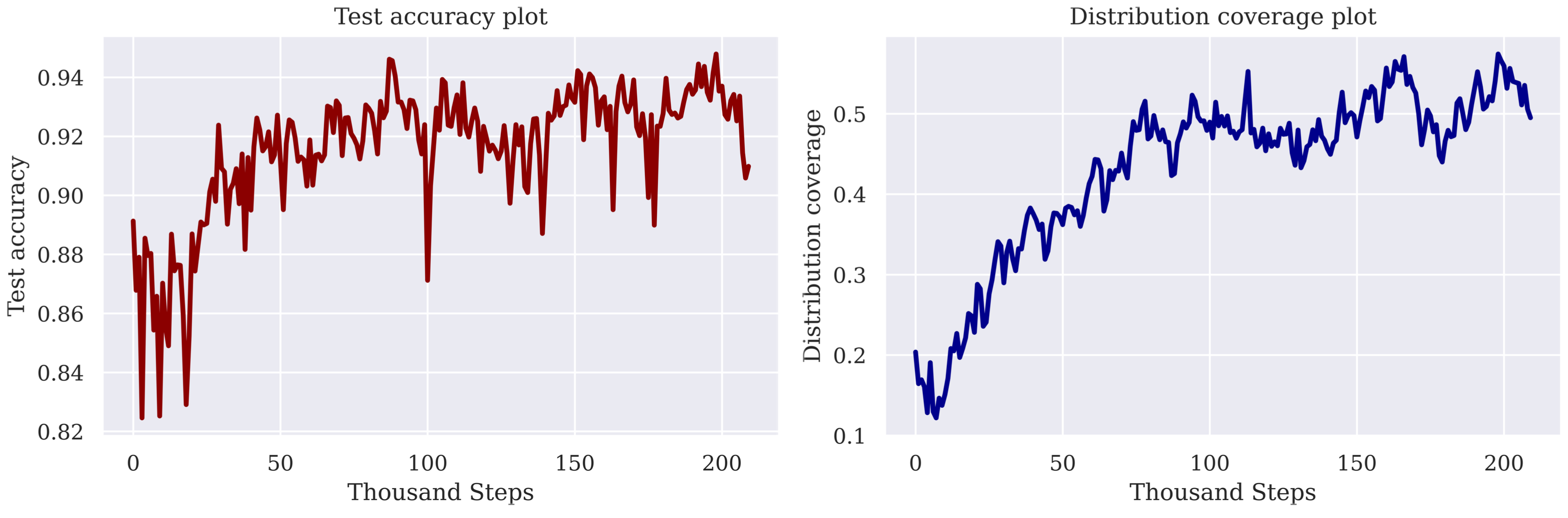
In Figure 4, Pearson correlation with target accuracy is 0.6066 for coverage versus 0.2565 for ordinary validation accuracy. The validation set shares the biased training distribution and is close to saturation. Coverage is a stronger empirical selection signal here, but remains an imperfect proxy.
4. Experiments
The method is tested with FiLM, Transparency by Design (TbD-net), and the Neuro-Symbolic Concept Learner (NS-CL) [30] [25] [24]. Baselines pretrain representations with a variational autoencoder (VAE) or SimCLR on exactly the same unlabeled images.
The comparison therefore evaluates different ways of using a shared unlabeled pool. It is not a comparison between DisCo with target data and baselines denied that data.
4.1. Datasets and implementation
CLEVR split A pairs cubes with gray/blue/brown/yellow and cylinders with red/green/purple/cyan; split B reverses these assignments. Spheres use all eight colors. Training includes either 0%, 0.1%, or 0.5% of objects from the reversed distribution.
The Ref dataset asks about attributes of referred objects, while OneHop adds relational questions. The original CLEVR compositional-generalization benchmark, CoGenT, contains more complex scenes and questions [13].
Backbones use their published implementations and hyperparameters. StyleGAN2 uses Adam at learning rate 0.002. The entropy threshold is chosen around the thirtieth percentile for the simpler datasets and the tenth percentile for CoGenT, where fewer random pairings satisfy presuppositions. Training uses one Titan RTX GPU.
4.2. Main results
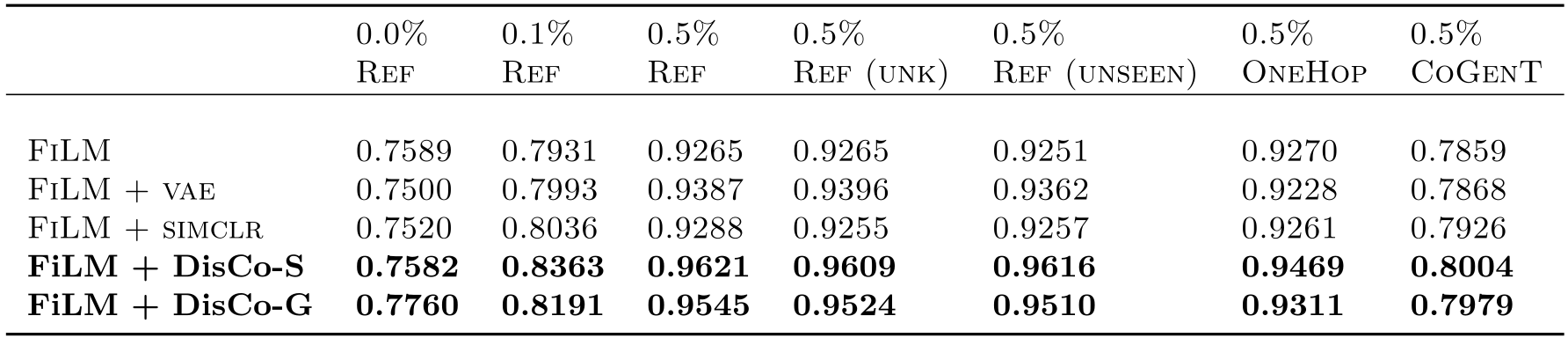
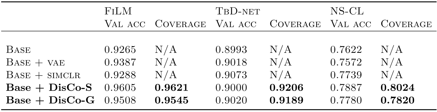
On 0.5% Ref, FiLM improves from 0.9265 to 0.9621 with direct sampling and 0.9545 with generated proposals. On the separately held-out image set, scores are 0.9251, 0.9616, and 0.9510 respectively. These unseen-image results support gains beyond reusing the exact adapted image pool.
Direct sampling also improves OneHop from 0.9270 to 0.9469 and CoGenT from 0.7859 to 0.8004. However, the fully biased 0% Ref case is an exception to universal improvement: DisCo-S scores 0.7582 versus the 0.7589 base, while DisCo-G reaches 0.7760.
The “unknown” condition uses a mixed unlabeled pool containing both split A and split B while testing on B. It relaxes exact target-distribution matching but still includes target combinations; it is not an arbitrary unrelated unlabeled distribution.
Other VQA backbones
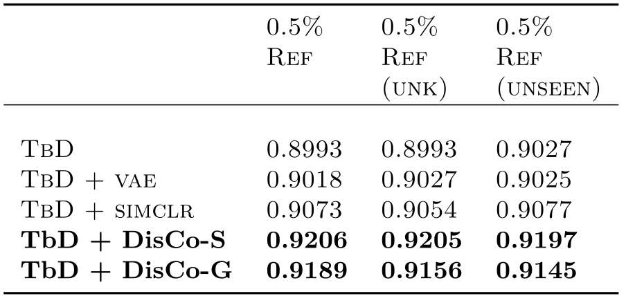
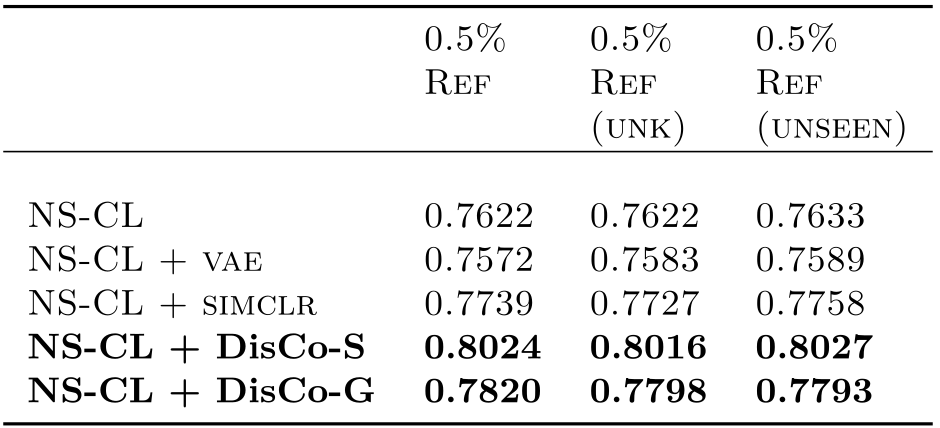
Tables 2 and 3 preserve all original, unknown-distribution, and unseen-image results. On 0.5% Ref, direct-sampling DisCo raises TbD-net from 0.8993 to 0.9206 and NS-CL from 0.7622 to 0.8024. Generated proposals also improve both, with smaller gains in these comparisons.
4.3. Component ablations
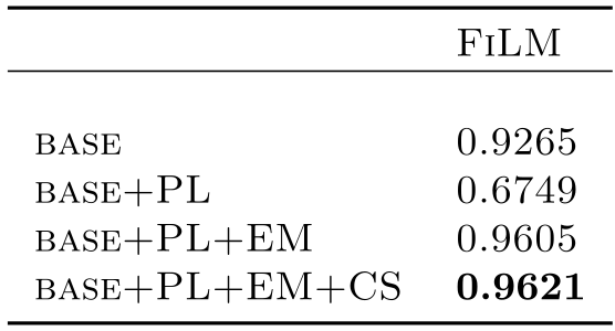
Unfiltered pseudo-labeling lowers FiLM accuracy from 0.9265 to 0.6749. Adding entropy filtering raises it to 0.9605, and coverage-based selection gives 0.9621. The large failure without filtering is central evidence that adding unlabeled pairs alone is insufficient.
Selection-strategy comparison
Table 5 isolates checkpoint selection within each DisCo run. For direct sampling, replacing validation-accuracy selection with coverage changes FiLM from 0.9605 to 0.9621, TbD-net from 0.9000 to 0.9206, and NS-CL from 0.7887 to 0.8024.
The authors do not apply this metric to VAE or SimCLR pretraining because those baselines do not construct pseudo-labels. Selection gains vary substantially across backbones.
4.4. Qualitative analysis
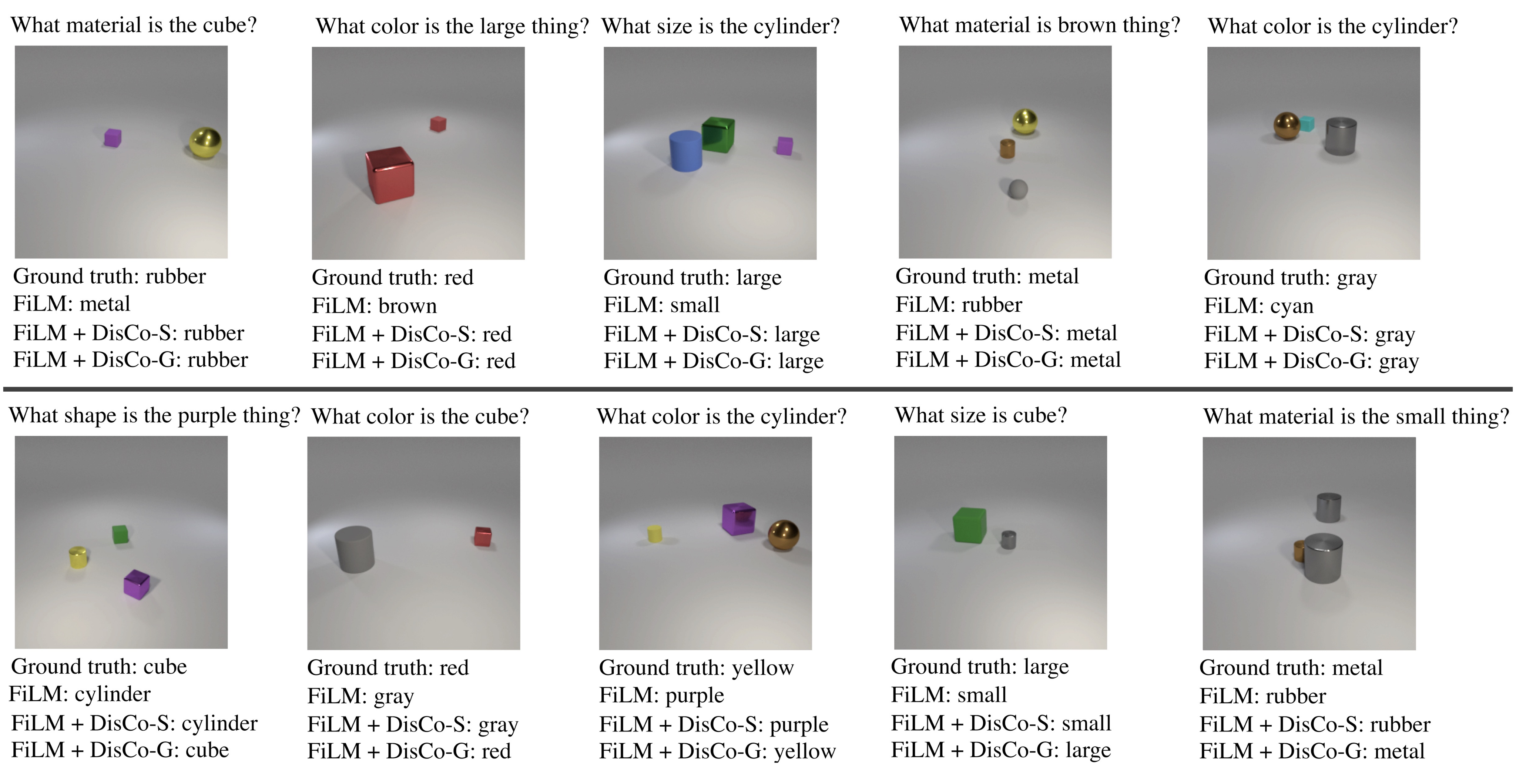
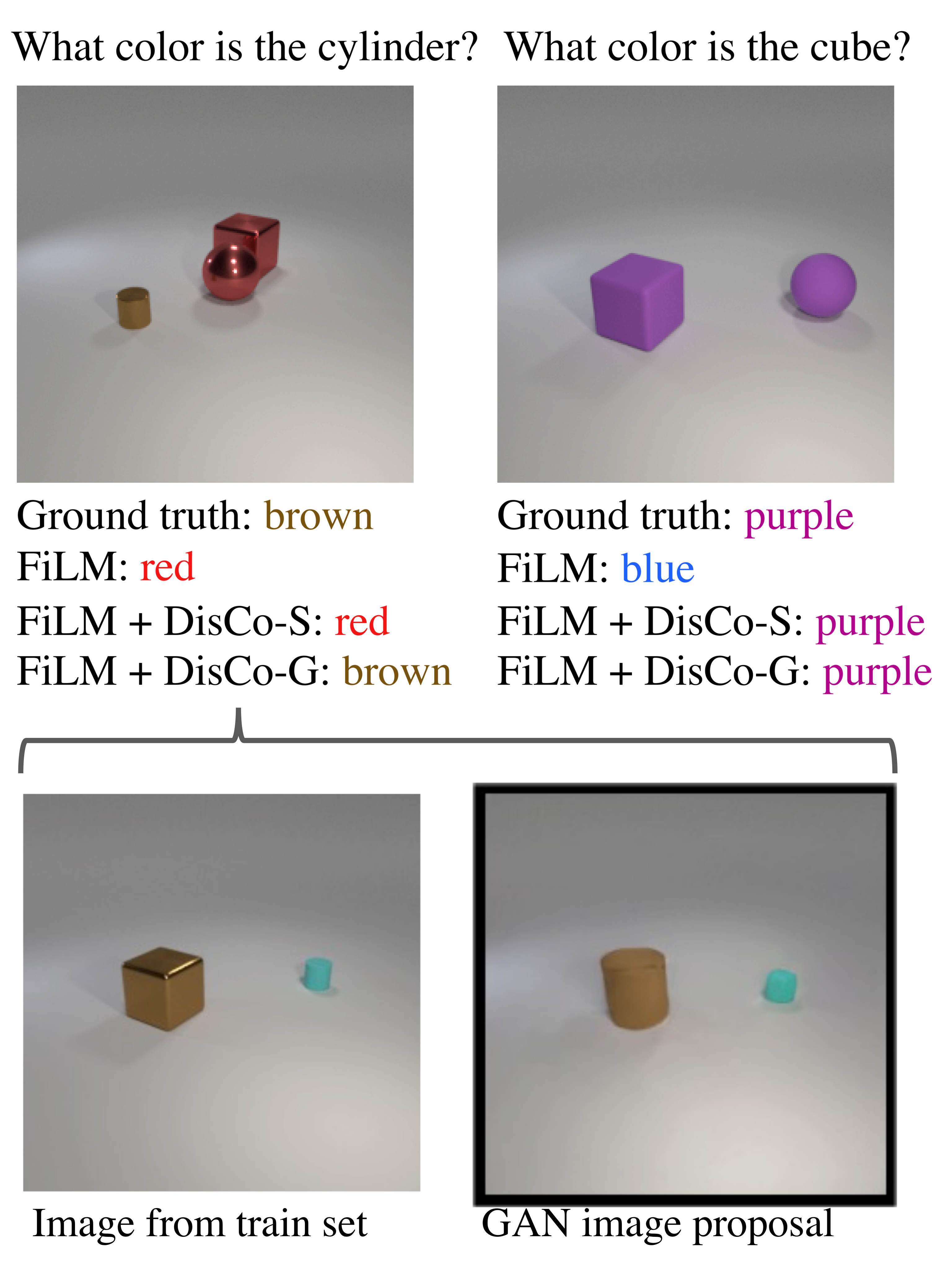
Figure 5 preserves successful and unsuccessful answers. In a brown-cylinder example, the base model and DisCo-S answer incorrectly, while DisCo-G answers correctly. A related generated scene motivates the hypothesis that generator diversity helps connect attribute combinations.
These examples illustrate a possible explanation, not an isolated causal test of why generated proposals improve the fully biased case.
Limitations
Bootstrapping relies on useful visual inductive biases and sufficiently correct initial predictions. Confidence can otherwise reinforce incorrect associations. The experiments use synthetic CLEVR scenes and do not establish performance on natural images, robot tasks, or much weaker initial models.
Coverage depends on the unlabeled pool itself. Missing relevant combinations cannot be repaired simply by maximizing confidence over a narrow pool, and the empirical correlation does not guarantee safe model selection under every shift.
5. Conclusion
The strongest result is a practical adaptation recipe: filter pseudo-labels for answerability and confidence, retain labeled supervision, and select using target-pool coverage. Across the evaluated backbones this improves several compositional benchmarks, while the fully biased direct-sampling exception and attribute-level regressions delimit the claim.
Broader impact
The paper emphasizes that an unlabeled dataset must itself cover relevant variation. Otherwise, self-training may inherit or amplify its biases despite requiring fewer labels.
Acknowledgments
The authors thank Eric Chan and acknowledge support from Stanford’s Institute for Human-Centered AI, Toyota Research Institute, the National Science Foundation, Office of Naval Research, and industrial sponsors. Joy Hsu acknowledges Knight-Hennessy and NSF graduate fellowship support.
Appendix A
All nine supplementary subsections are retained, with complete proposal examples, threshold tests, coverage stress tests, unknown-distribution comparisons, and per-attribute results.
A.1. Code
The released DisCo implementation builds on the FiLM codebase. The authors again caution that adequate unlabeled-data coverage is necessary.
A.2. Dataset construction
The generated Ref and OneHop data use two or three objects per scene. Split A has 8,000 training images and 2,000 validation images; split B has 2,000 target images. A further 8,000-image set evaluates unseen images from the same target distribution.
A.3. Proposal examples
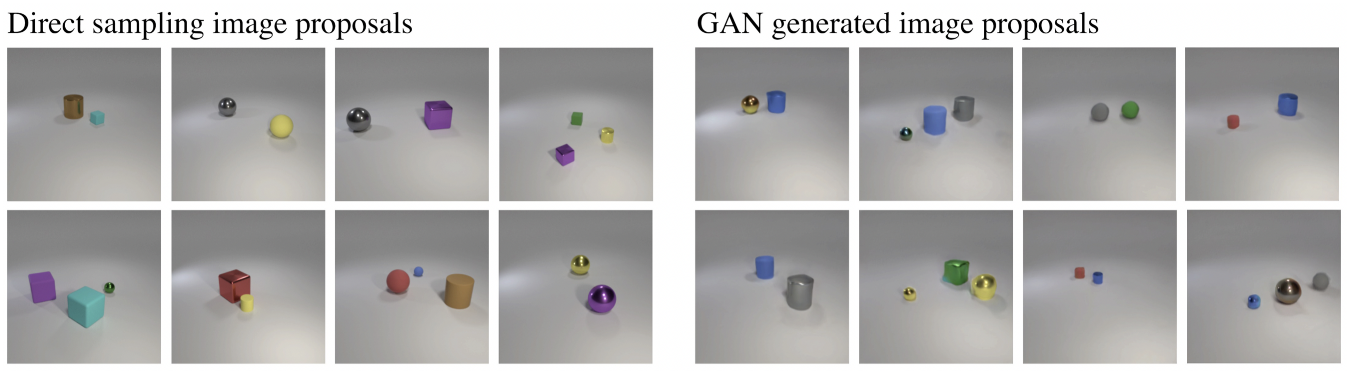
Figure 6 retains sixteen example images from direct sampling and GAN generation, showing the range of proposed attribute combinations. Their visual diversity is illustrative rather than a quantitative guarantee of complete distribution coverage.
A.4. Entropy thresholds
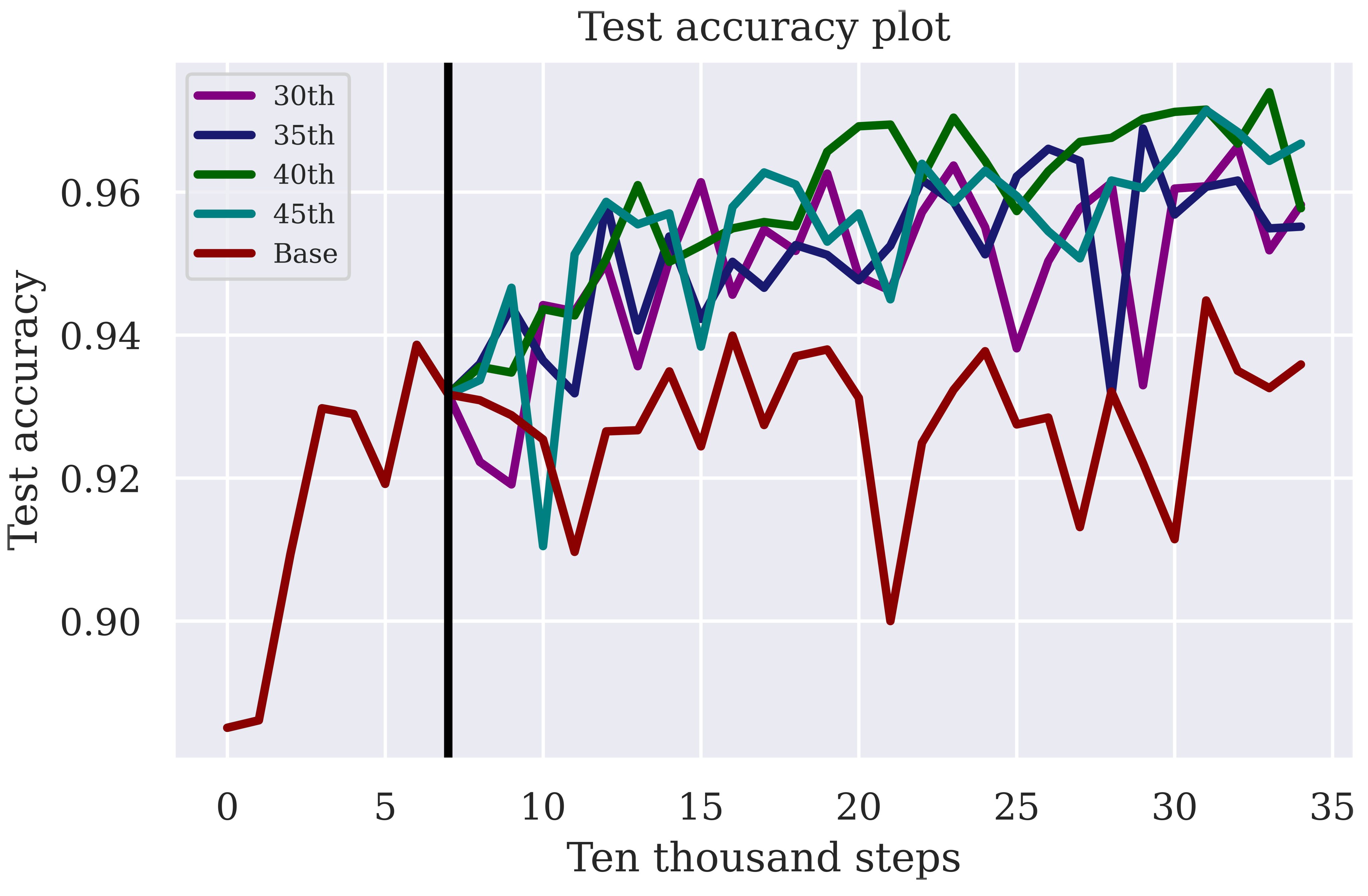
Table 6 reports 0.9612, 0.9616, 0.9667, and 0.9643 for entropy percentiles 30, 35, 40, and 45 on 0.5% Ref. Figure 7 retains the full accuracy trajectories and pseudo-labeling onset marker.
Runs vary both random seed and threshold. Their consistent improvements indicate some robustness, but the table does not isolate threshold effects from seed variability or provide repeated-run uncertainty for each threshold.

A.5. Coverage under degradation
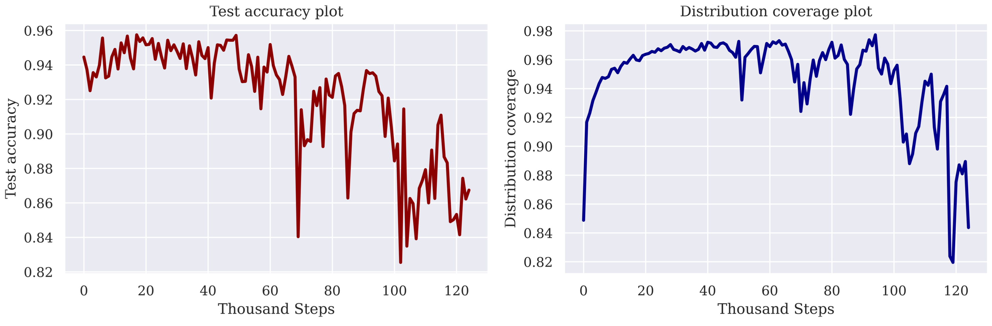
Figures 8 and 9 preserve cases where performance degrades. Coverage tracks accuracy with reported correlations 0.6585 and 0.7987, including a high-threshold run that fails substantially.
The proposed explanation is that conflicting labeled and pseudo-labeled supervision reduces confidence, thereby rejecting more candidate pairs. This is an empirical observation in the examples, not proof that erroneous labels cannot propagate.
A.6. Unknown distributions
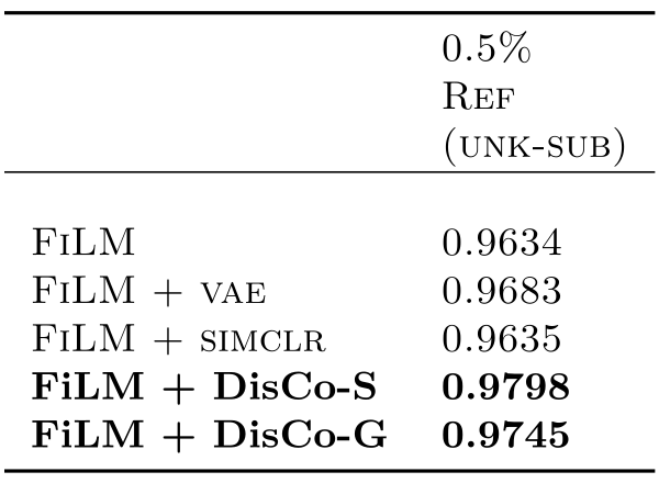
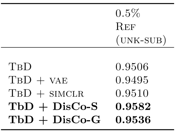
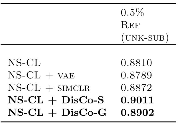
The supplementary “unknown-subset” setting trains on labeled A, adapts with unlabeled B, and evaluates on the full A+B distribution. Tables 7–9 retain all comparisons. Direct sampling improves FiLM from 0.9634 to 0.9798, TbD-net from 0.9506 to 0.9582, and NS-CL from 0.8810 to 0.9011.
This tests an unlabeled pool narrower than the evaluation distribution, complementing the main unknown condition’s broader pool.
A.7. Baseline implementation
VAE and SimCLR baselines start from ResNet101 image features, add convolution, batch normalization, and LeakyReLU layers, and train with feature reconstruction or contrastive objectives. Their trained encoders then initialize additional visual encoding for the VQA models.
A.8. Attribute-level results
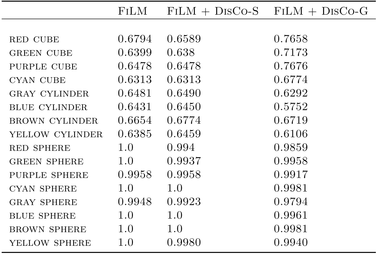
Table 10 retains every color–shape row. GAN proposals improve unseen cubes but lower several cylinder accuracies: blue cylinders fall from 0.6431 to 0.5752, and yellow cylinders from 0.6385 to 0.6106. Several sphere results also decrease slightly.
Thus aggregate improvement is not uniform compositional mastery. Different combinations benefit or regress, even in the best overall fully biased model.
A.9. Additional examples
Figure 10 retains five examples spanning low-entropy correct answers, valid but incorrectly answered questions, and a missing-referent failure. Figure 11 retains ten additional comparisons among the base model and both proposal variants, including successes unique to generated proposals.