At a glance
RoboKit combines GPU-parallel numerical optimization, geometry queries, differentiable rendering, physics rollouts, and policy training in one robotics toolkit. Multi-seed solvers and task-specific optimizers provide the numerical core; learned policies can amortize repeated optimization.
The reported gains span seven solver tasks, four distilled-policy tasks, and six reinforcement-learning tasks. Speedups depend on the workload and protocol. The complete figures, tables, residual definitions, algorithms, and appendix results are retained below.
1. Introduction
Optimization remains useful inside teleoperation, data generation, model-based control, and learned policies [1] [7] [12]. RoboKit aims to make these uses faster while allowing costs and solvers to be recombined.
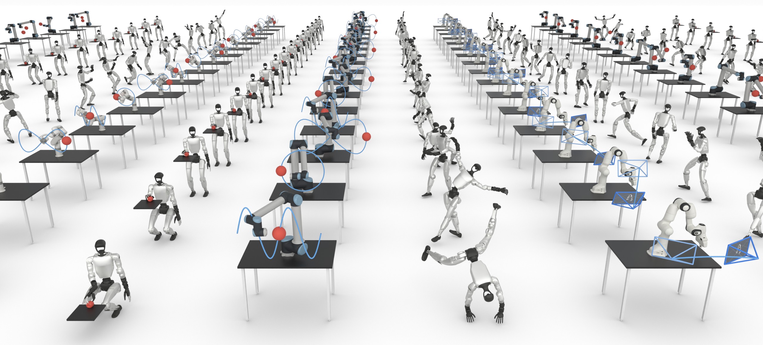
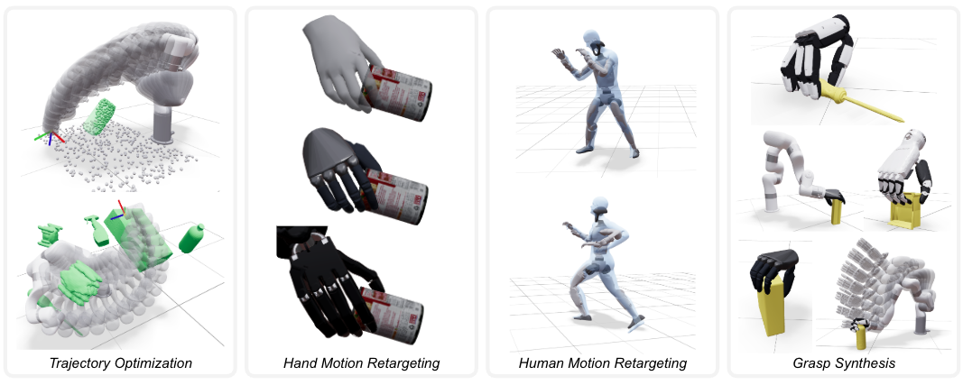
Its three design choices are parallel sampling plus multiple numerical solvers; accelerated geometry/rendering/physics; and differentiable costs usable as policy-training losses. Figure 1 illustrates the task range.
Optimization libraries
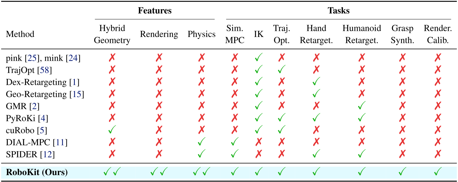
Table 1 preserves the authors’ feature comparison. The distinction is coverage of contact-oriented geometry, rendering, physics, and learning in one toolkit, beyond collision-free motion generation or kinematics alone. This is the paper’s comparison of the evaluated software, not a timeless feature inventory.
3. Method
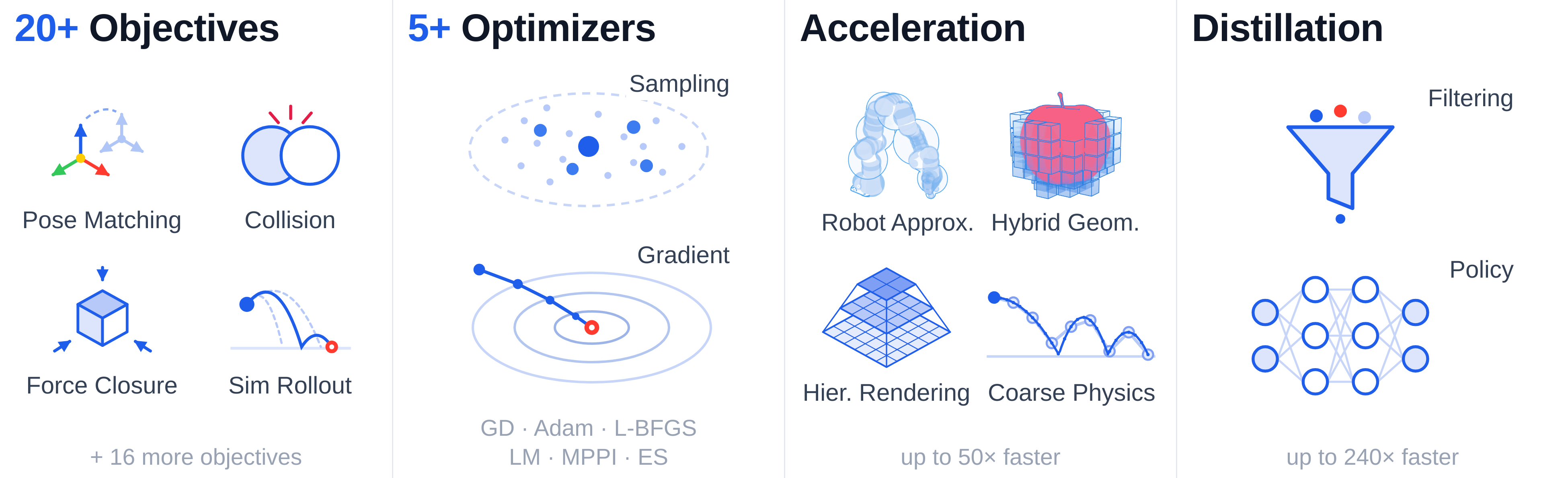
The pipeline first samples and refines candidate solutions, accelerates expensive geometric or simulation evaluations, and optionally trains a policy from solved examples or direct cost gradients. Figure 2 retains the complete architecture.
3.1 Parallel solver
Variables include joint configurations, trajectories, rigid poses, and auxiliary scales. Supported joints are fixed, revolute, prismatic, and mimic; differentiable forward kinematics supplies poses and Jacobians.
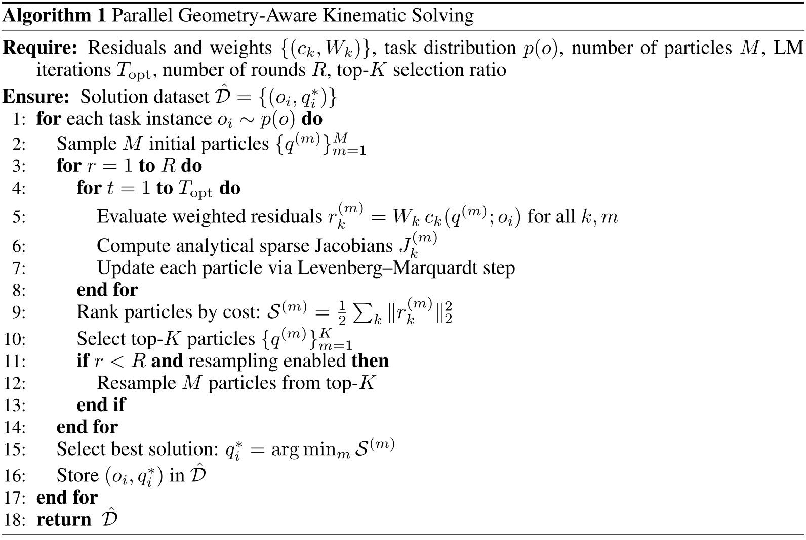
Warp implements particle sampling, selection, distribution fitting, and resampling, combined with gradient descent, Adam, L-BFGS, Gauss–Newton, Levenberg–Marquardt, or MPPI. Sparse coordinate-format Jacobians support larger problems. Costs are weighted squared residuals with analytic derivatives where available. Physics rollouts can instead be scored by gradient-free sampling [17] [19].
3.2 Acceleration structures
The expensive operations are collision geometry, rendered-image comparison, and simulator stepping. RoboKit uses spatial pruning and stages computation from coarse to fine.
Hybrid geometry
A precomputed voxel SDF supplies cheap distances away from an object; queries within a threshold switch to its mesh. The threshold is four voxel widths by default. This improves near-contact geometric detail without paying for a mesh query everywhere. The grasp-speed ablation below specifically uses voxel-only optimization, which must be distinguished from this hybrid option.
Equation

Coarse-to-fine collision queries
One bounding sphere encloses each link’s collision spheres. When that sphere lies beyond the safety margin, one broad query prunes the entire link; otherwise the individual spheres are checked. The retained piecewise formula specifies the effective distance used by the collision residual.
Equation

Coarse-to-fine rendering
Calibration begins with many seeds, low-resolution masks, and strong blur. Later stages keep promising seeds, increase image resolution, and remove blur. The schedule makes early exploration cheaper and smoother, then refines the silhouette fit.
Coarse-to-fine physics
Early optimization stages can use larger simulator timesteps, fewer solver iterations, and fewer collision pairs, then switch to full physics. This describes the toolkit’s coarse-to-fine capability; the benchmark comparisons must still be read under their individual matched-task protocols.
3.3 Policy learning
Distillation either imitates optimized configurations or directly minimizes the original task costs through the policy output. These are complementary training routes.
Offline distillation
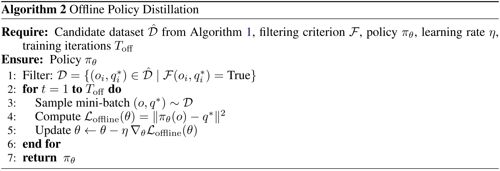
Solve sampled task instances, optionally reject poor or physically unsuccessful solutions, then regress policy outputs onto retained configurations. The exact squared-error objective is preserved. Filtering is especially important when grasp optimization produces many failures.
Equation

Online distillation
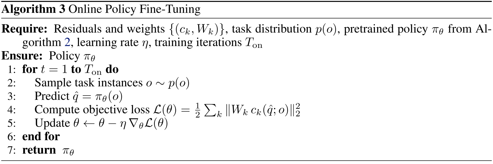
Sample fresh task inputs and backpropagate the weighted residual loss through the policy. This differentiates the cost evaluated at the predicted configuration; it does not unroll or differentiate the numerical solver. “Online” here describes fresh training instances and current-policy outputs, not necessarily interaction with physical hardware.
Equation

Hybrid distillation
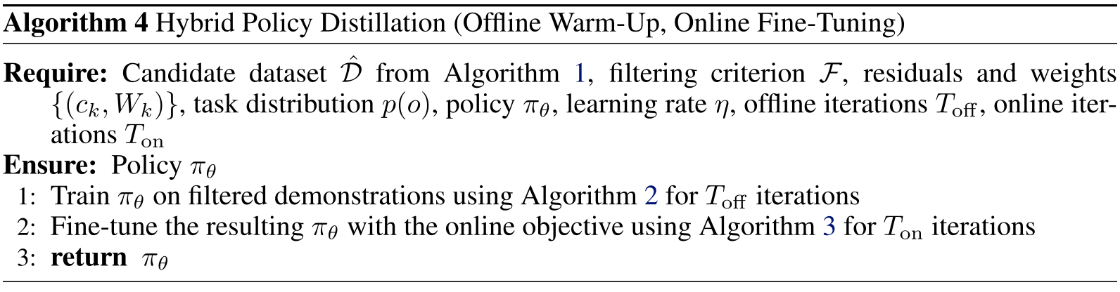
Direct objective training works well on simpler retargeting but can converge poorly or diverge on nonconvex grasp tasks. The hybrid procedure first learns filtered demonstrations, then fine-tunes with direct objective gradients.
4. Experiments
The evaluation separates solver speed/quality, distilled-policy performance, reinforcement-learning training time, and component ablations. Appendix A gives success definitions and hardware; Appendix B includes batch scaling and additional baselines.
4.1 Experimental settings
The main solver benchmark runs on one RTX 4090. Most times average five warmed-up runs; human retargeting uses three runs and hand retargeting one pass over all frames. Tasks cover Panda kinematics/planning/calibration, Shadow Hand retargeting, G1 retargeting, MANO grasp synthesis, and physics-based retargeting across five hands.
Policy-distillation comparisons use an RTX A5000 and their own evaluation workloads. Their optimizer rows must not be combined with the main table to infer additional speedups.
4.2 Solver performance
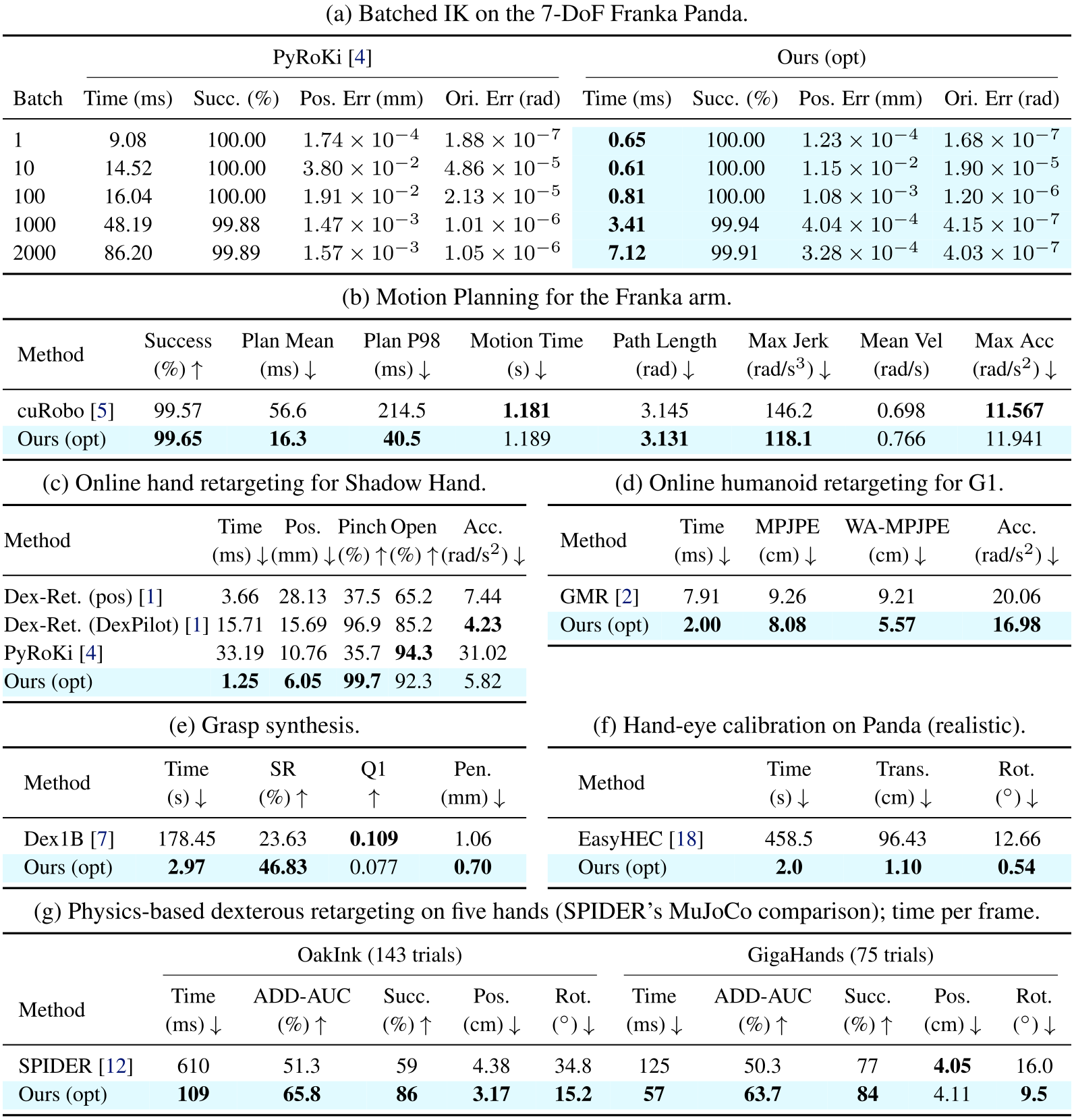
Table 2 retains all seven comparisons. At IK batch 2,000, RoboKit takes 7.12 ms versus PyRoKi’s 86.20 ms with approximately 99.9% success. Both use LM with 64 seeds reduced to four and sixteen iterations; the comparison reflects implementation and solver settings.
For motion planning, mean time falls from cuRobo’s 56.6 to 16.3 ms, with similar success. Path length and jerk improve, while motion duration and maximum acceleration are slightly higher. Obstacles are primitive boxes, so this test does not exercise hybrid mesh geometry.
Hand retargeting improves position and pinch metrics at 1.25 ms, but does not lead every smoothness/open-hand metric. Human retargeting takes 2.00 versus GMR’s 7.91 ms with lower reported position errors.
For 4,096 grasps, voxel optimization takes 2.97 versus Dex1B’s 178.45 s and raises simulated success from 23.63% to 46.83%; Dex1B has higher Q1. On noisy calibration with 35 cm/45° initial error, RoboKit reaches 1.10 cm/0.54° in 2 s while EasyHEC fails to converge. The separate easy split yields the reported 57× speedup.
Physics-based retargeting improves object ADD-AUC on OakInk and GigaHands while reducing time 5.6× and 2.2×. GigaHands position error is slightly worse. Appendix A explains the excluded trials and use of released baseline rollouts.
4.3 Policy learning performance
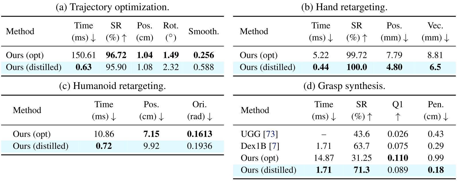
Table 3 reports offline-trained policies under separate RTX A5000 protocols. Trajectory inference falls from 150.61 to 0.63 ms per frame, but success changes from 96.72% to 95.90%, orientation error increases, and the smoothness metric worsens. Human retargeting is about fifteen times faster with larger position/orientation errors.
The hand policy improves its reported errors as well as latency. The grasp policy reaches 71.3% success versus 63.7% for learned Dex1B and 31.25% for this table’s optimizer, with lower penetration. These are different workloads and units from Table 2; Table 3 grasp penetration is in centimeters. Figure 3 preserves all qualitative examples.
Reinforcement learning
On the same MuJoCo Warp physics, RoboKit trains PPO on six mjlab tasks with 4,096 environments. Table 4 reports minutes to 95% and 100% of mjlab’s final score, using medians over five seeds. The 100% targets are reached about 1.3–2.1 times sooner. This measures time to a chosen score, not an improvement in final task score.

4.4 Distillation ablations
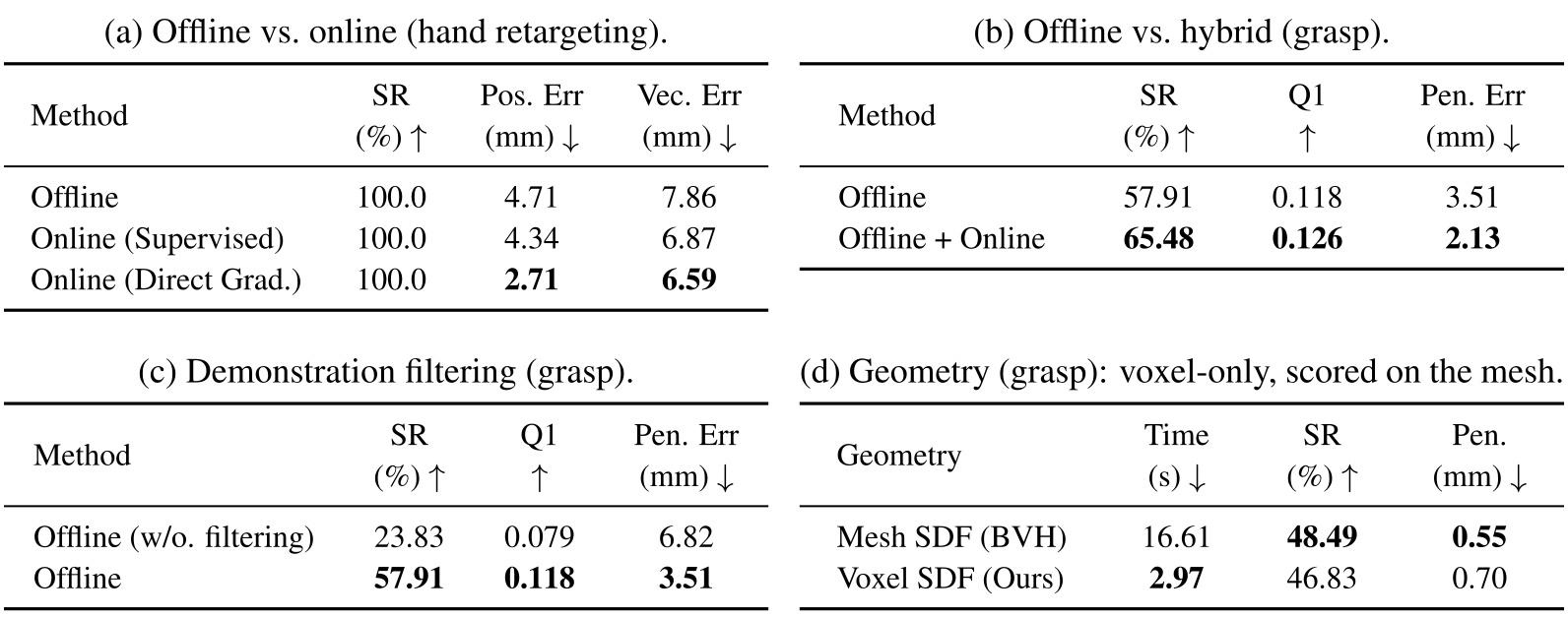
For random-configuration hand retargeting, direct objective training lowers position error from offline learning’s 4.71 to 2.71 mm. Fresh solver-supervised targets achieve 4.34 mm. These ablation inputs differ from the DexYCB motion evaluation.
For grasping, offline initialization plus online refinement raises success from 57.91% to 65.48% and reduces penetration. Removing demonstration filtering lowers offline success to 23.83%. The evidence favors high-quality initialization on the harder nonconvex task, not direct-gradient training universally.
Geometry representation
Replacing mesh queries with voxel-only queries reduces grasp solve time from 16.61 to 2.97 s. Success drops from 48.49% to 46.83% and penetration increases from 0.55 to 0.70 mm. All grasps are evaluated against the mesh. These are measured speed–quality tradeoffs.
Solver components
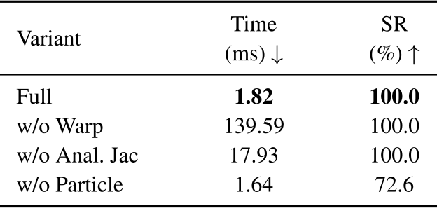
Table 6 isolates implementation choices on one Panda IK setting. Replacing Warp with PyTorch kernels increases latency from 1.82 to 139.59 ms; numerical Jacobians increase it to 17.93 ms. Removing multi-seed sampling saves little time but reduces success from 100% to 72.6%.
5. Conclusion
The paper demonstrates a reusable optimization toolkit that combines efficient numerical kernels, geometric representations, and policy training across several robot tasks. Its strongest evidence is workload-specific throughput with explicit quality measures, rather than a claim that every task or metric improves.
6. Limitations
RoboKit targets GPU-parallel workloads. The authors expect a C++ CPU solver to be preferable for single-instance CPU kinematics. There is no trajectory graph-search stage, the evaluated benchmarks do not strongly stress that omission, and inverse dynamics is unsupported.
Differentiable costs and good simulation scores do not establish global optimality, physical grasp guarantees, or general safety. The appendix also notes derivative discontinuities at geometric representation switches.
Acknowledgment
The authors acknowledge NSF CAREER IIS-2240014 and NSF CCF-2112665/TILOS support.
Appendix
The complete supplement covers experimental protocols, additional results, all mathematical residual definitions, four algorithms, and the final qualitative montage. The project page links further video demonstrations.
A. Experimental details
Appendix A defines workloads, metrics, hardware, and baselines needed to interpret the reported timings.
A.1 Hardware and profiling
The default system pairs an RTX 4090 with an Intel Xeon Gold 5120 at 2.20 GHz. Warmup compiles and caches kernels. Unless stated otherwise, timing is total wall-clock solve time for the full batch, with five runs.
A.2 Task definitions
IK succeeds below 5 mm position error and 0.05 rad orientation error; its tabulated errors are 98th percentiles over successful instances. Planning additionally checks world/self collision, dynamics, and joint limits on 25 ms interpolation, with the original 0.2 rad joint-limit tolerance. Planning statistics condition on successful plans.
Hand retargeting uses 501 right-hand DexYCB captures. Humanoid retargeting uses 44 AMASS/SFU sequences; its world-aligned error applies one similarity alignment per 100-frame segment. Grasp synthesis uses 128 scenes, 32 grasps each, and 24 seeds per grasp. Success requires penetration at most 5 mm and passing ManiSkill’s external-force test.
Physics retargeting scores 218 of 248 released trials: thirty fail SPIDER’s own export check. It uses released scenes/retargets across five hands, seven OakInk tasks, three GigaHands clips, and five seeds. Baseline accuracy comes from released rollouts.
RL tasks reuse mjlab rewards, commands, observations, randomization, terminations, and curricula, checked on identical states. One evaluator scores both methods. These protocol details constrain interpretation of the reported speedups.
A.3 Baselines
PyRoKi and cuRobo provide GPU kinematics/planning baselines; Dex-Retargeting and GMR are single-instance retargeting comparisons. Dex1B supplies grasp protocols and a learned comparator; UGG and GeoRT supply learned grasp/hand baselines. EasyHEC handles calibration, SPIDER and DIAL-MPC physics-based optimization, and mjlab policy training. Pinocchio and Pink are the CPU Python-example comparisons.
B. Additional experiments
Appendix B extends the solver and learned-policy comparisons and reports means with population standard deviations where specified.
B.1 Batch scaling: inverse kinematics
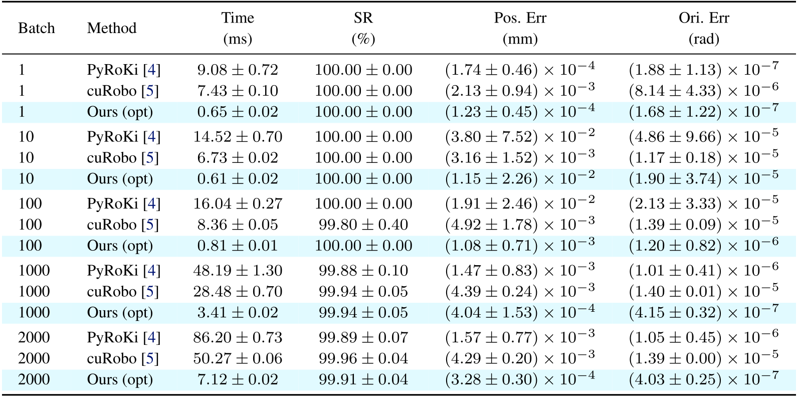
Table 7 includes cuRobo and PyRoKi at batches one through 2,000. RoboKit is 7.1–11.5 times faster than cuRobo in these runs, with similar success and generally smaller errors. Timing covers the full batch; error statistics include only successful instances.
Other batched tasks
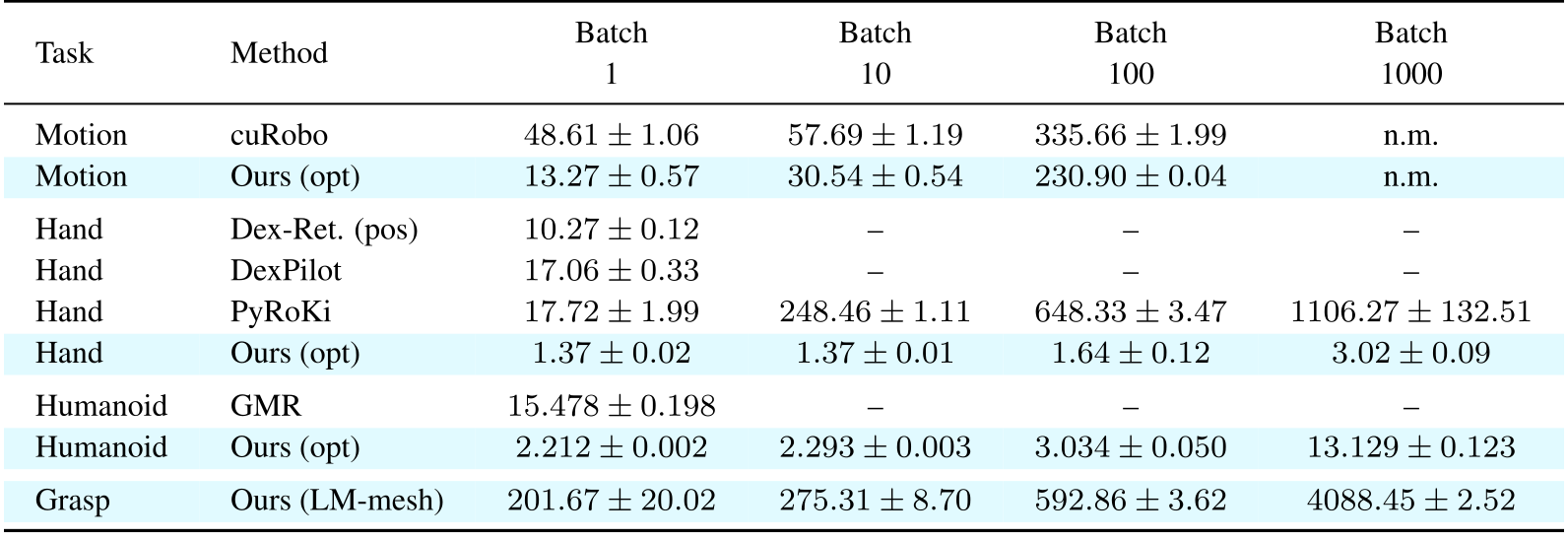
Hand retargeting grows from 1.37 to 3.02 ms as batch size increases from one to 1,000; humanoid retargeting grows from 2.21 to 13.13 ms. These are simultaneous-stream frame latencies. Motion and grasp timings instead cover complete batches.
The sweep differs from Table 2. Motion planning uses four candidates per query and disables cuRobo’s graph search. Dashes mean no batched API; “n.m.” means unmeasured, not failure.
B.2 Learned policy comparison
On DexYCB, the distilled hand policy lowers unaligned fingertip error from GeoRT’s 37.4 to 23.0 mm and 95th-percentile error from 58.5 to 29.9 mm. Procrustes-aligned error also improves. The retained table preserves all three definitions.

B.3 Locomotion comparison
On Go2 trotting, ten sequential random jumps, and twenty crate-climbing trials, RoboKit uses the released DIAL-MPC models/rewards/settings but 0.6 times as many samples. Table 10 reports 2.1×, 2.3×, and 8.3× faster control steps with matched or better task scores. Crate success is 80% versus 75%, on ten heights and two seeds each.

B.4 Grasp synthesis ablation
Table 11 crosses LM/gradient descent with mesh/voxel geometry for 4,096 grasps. LM uses 64 iterations, while annealed gradient descent uses 6,000. Reported times cover optimizer iterations; all success evaluations use the full physical grasp test.
The appendix’s LM-SDF Q1 is 0.0666, whereas Table 2 lists 0.077 for its voxel result. The paper does not explain that difference; both original tables are retained without silently reconciling the values.

B.5 CPU inverse-kinematics baselines
The single-instance comparison uses official Pinocchio and Pink Python examples. RoboKit still runs sampling and LM on the GPU. Joint-limit enforcement also differs: the default Pinocchio example lacks it. The result supports this implementation-level comparison, not superiority over optimized CPU solvers in general.

C. Implementation details
Appendix C retains the exact original residuals, inline derivative definitions, boundary conventions, and complete algorithms.
C.1 Analytic objectives
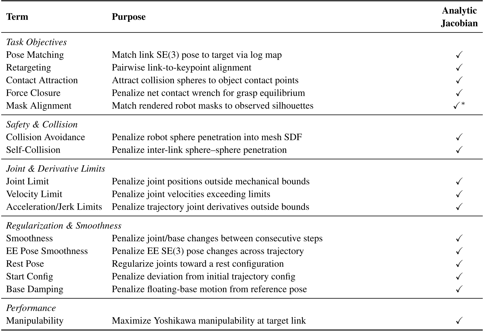
Table 13 lists all built-in objective families. Mask alignment combines analytic projection derivatives with central-difference image gradients; the other listed terms use analytic Jacobians. Batched evaluation is available throughout.
Weighted residual objective
The solver minimizes weighted squared residuals. Each diagonal weight combines a task gain in (0,1] with per-dimension weights. The original mathematical definition is retained.
Equation

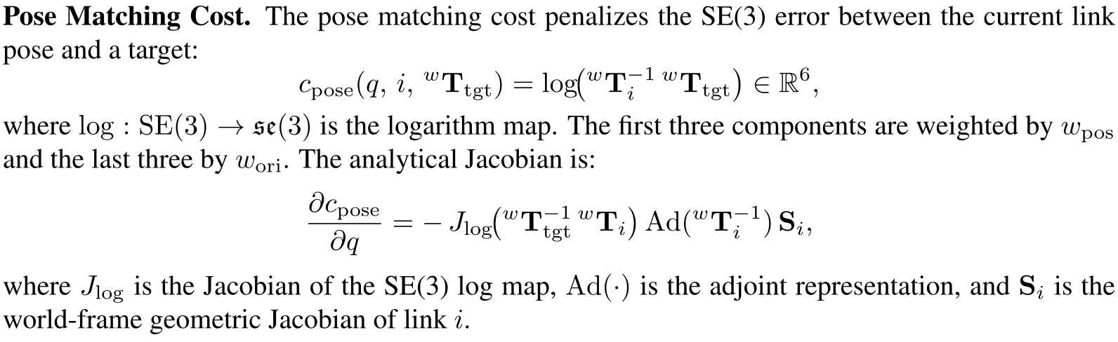
Pose matching
Pose matching uses a six-dimensional rigid-pose logarithm and separate position/orientation weights. The retained definition includes the exact logarithm Jacobian, adjoint, and world-frame geometric Jacobian.
Equation
Retargeting
Relative keypoint displacement is compared across embodiments with scale factor s. An optional angular term compares vector directions. The complete displacement residual is preserved below.
Equation

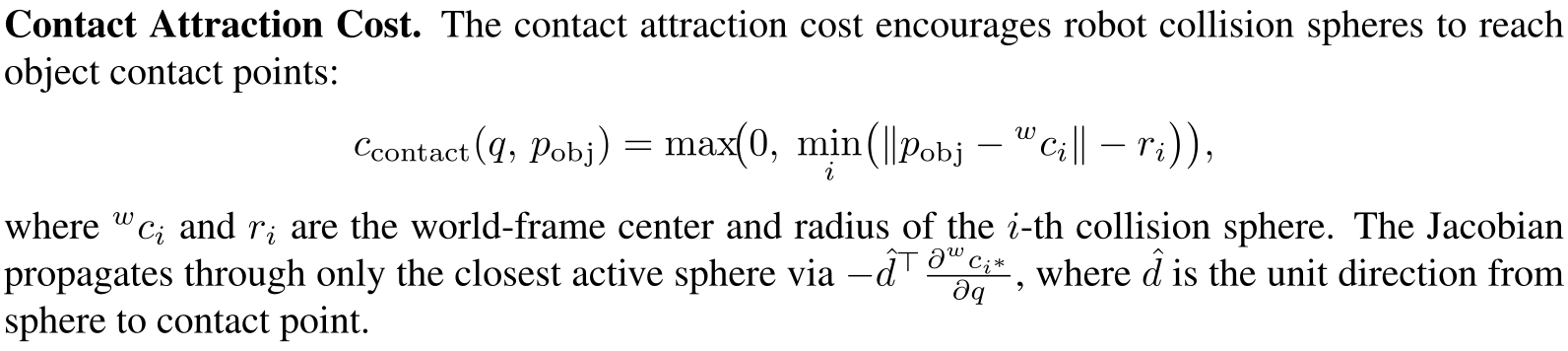
Contact attraction
A contact point is attracted to its closest active collision sphere. Only that sphere contributes the local Jacobian. The original residual and derivative definition are retained together.
Equation
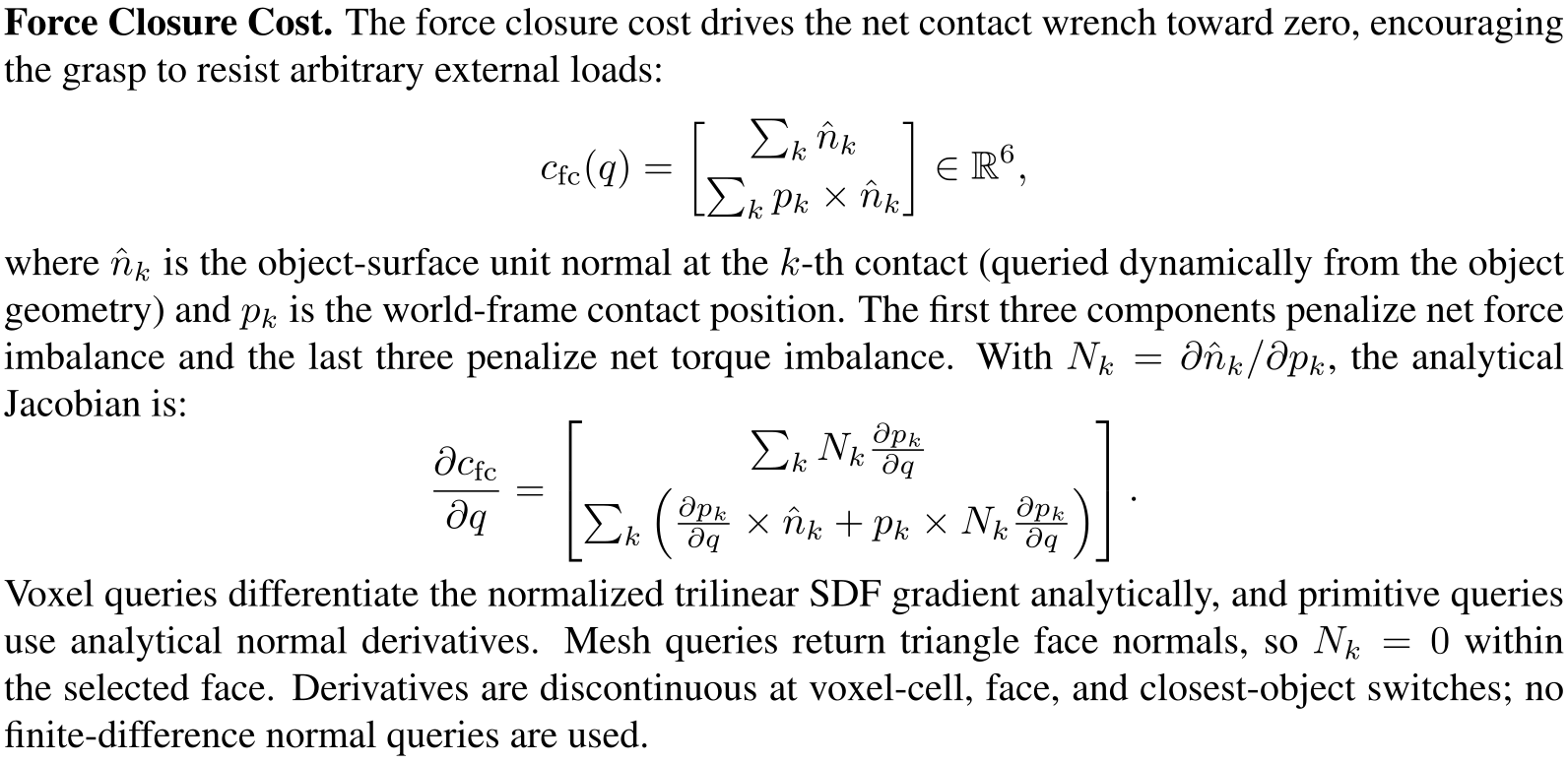
Force closure
The residual penalizes summed contact normals and their moments. Voxel normals use differentiated normalized trilinear gradients; mesh normals are constant within a selected triangle. Cell, face, and closest-object switches create derivative discontinuities. A low net-wrench residual alone is not a proof of force closure.
Equation
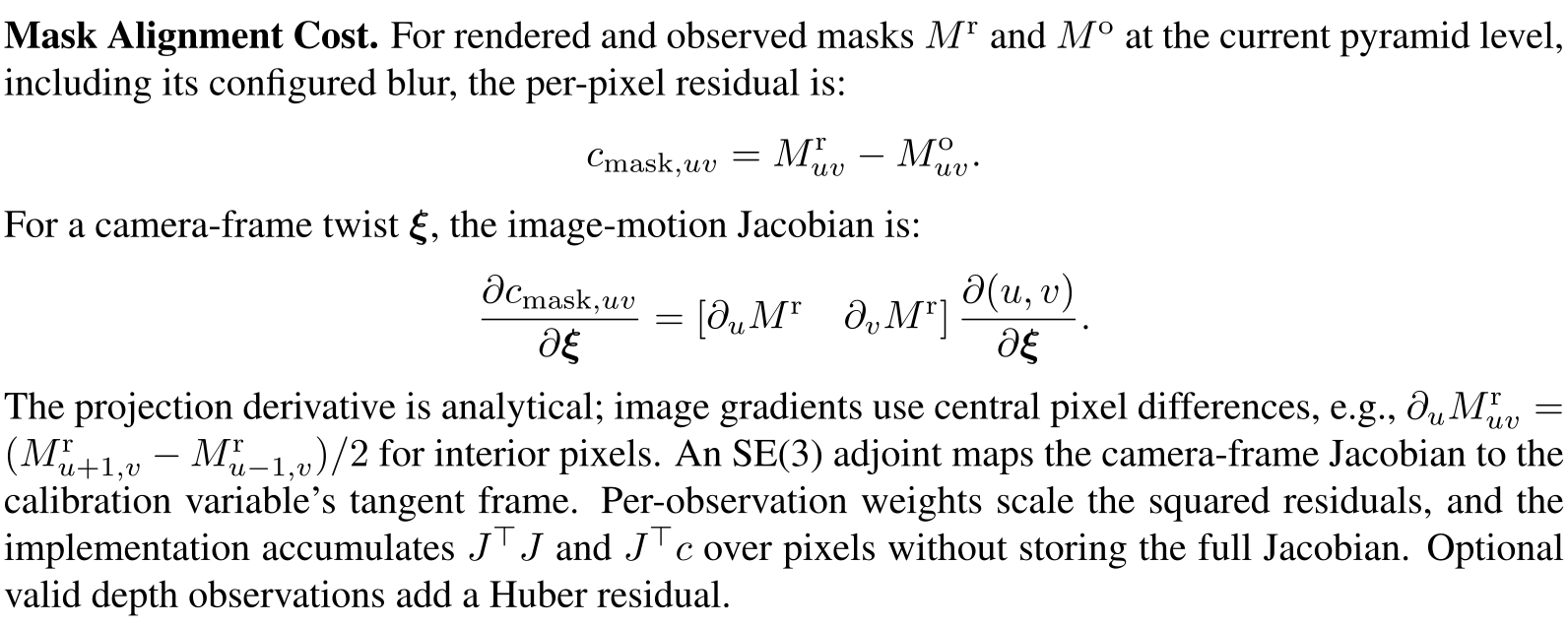
Mask alignment
Mask residuals compare rendered and observed silhouettes at the current blur/resolution level. Projection derivatives are analytic, image derivatives use central pixel differences, and the system accumulates normal equations without storing the full pixel Jacobian. Optional depth measurements add a Huber residual.
Equation
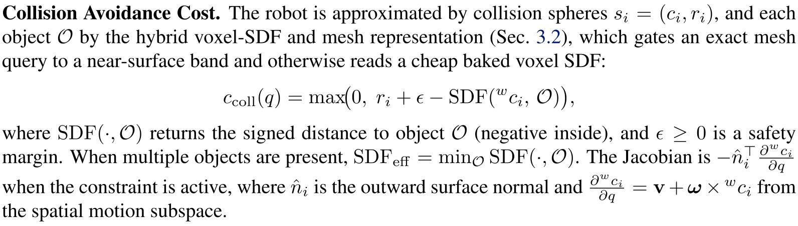
Collision avoidance
Sphere penetration is measured against the nearest object’s signed distance, including a safety margin. The original active-residual Jacobian and spatial-motion definition are preserved.
Equation
Self-collision
For selected non-adjacent links, sphere overlap generates a penalty. Its Jacobian uses the direction between centers and their relative kinematic derivatives.
Equation

Joint limits
Soft residuals penalize positions outside mechanical bounds. The original definition also gives the available hard quadratic-program constraints on a step.
Equation

Velocity limits
A finite-difference velocity residual penalizes excess speed, with the sign-dependent derivative active only outside the limit.
Equation

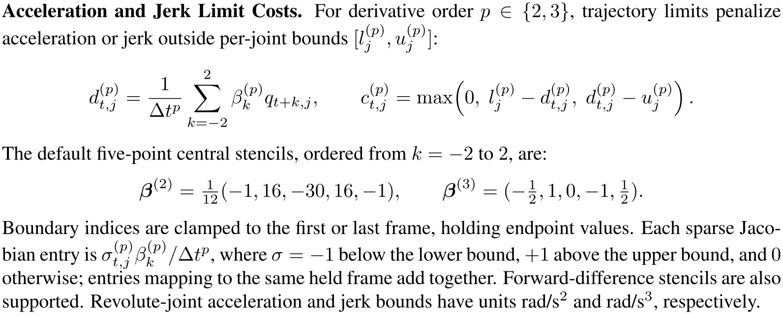
Acceleration and jerk limits
Acceleration and jerk use five-point central stencils by default. Endpoint indices clamp to the first/last frame, and repeated sparse entries add. The retained definition includes both stencil coefficient vectors, bound residuals, Jacobian signs, and the supported forward-difference alternative.
Equation
Joint and base smoothness
Adjacent joint differences provide regularization. Floating bases add a pose-logarithm term with its adjoint-based Jacobian.
Equation

End-effector pose smoothness
An end-effector pose-logarithm residual penalizes changes between successive trajectory frames.
Equation

Rest pose
Joint configurations are regularized toward a preferred pose; floating bases additionally receive a rigid-transform residual.
Equation

Start configuration
The first trajectory configuration is penalized for departing from the specified initial configuration.
Equation

Base damping
Floating-base damping penalizes rigid-pose displacement from a reference.
Equation

Manipulability
The reciprocal of a regularized Yoshikawa translational manipulability measure becomes a cost. The exact determinant expression and analytic-gradient construction are retained.
Equation

C.2 Algorithms
Algorithm 1 shows sampled multi-round LM refinement and top-particle selection. Algorithm 2 filters solved examples before supervised training. Algorithm 3 trains from fresh task samples through differentiable residuals. Algorithm 4 sequences the offline warmup and online refinement. All requirements, loops, indices, and update formulas are preserved.
D. Additional visualization
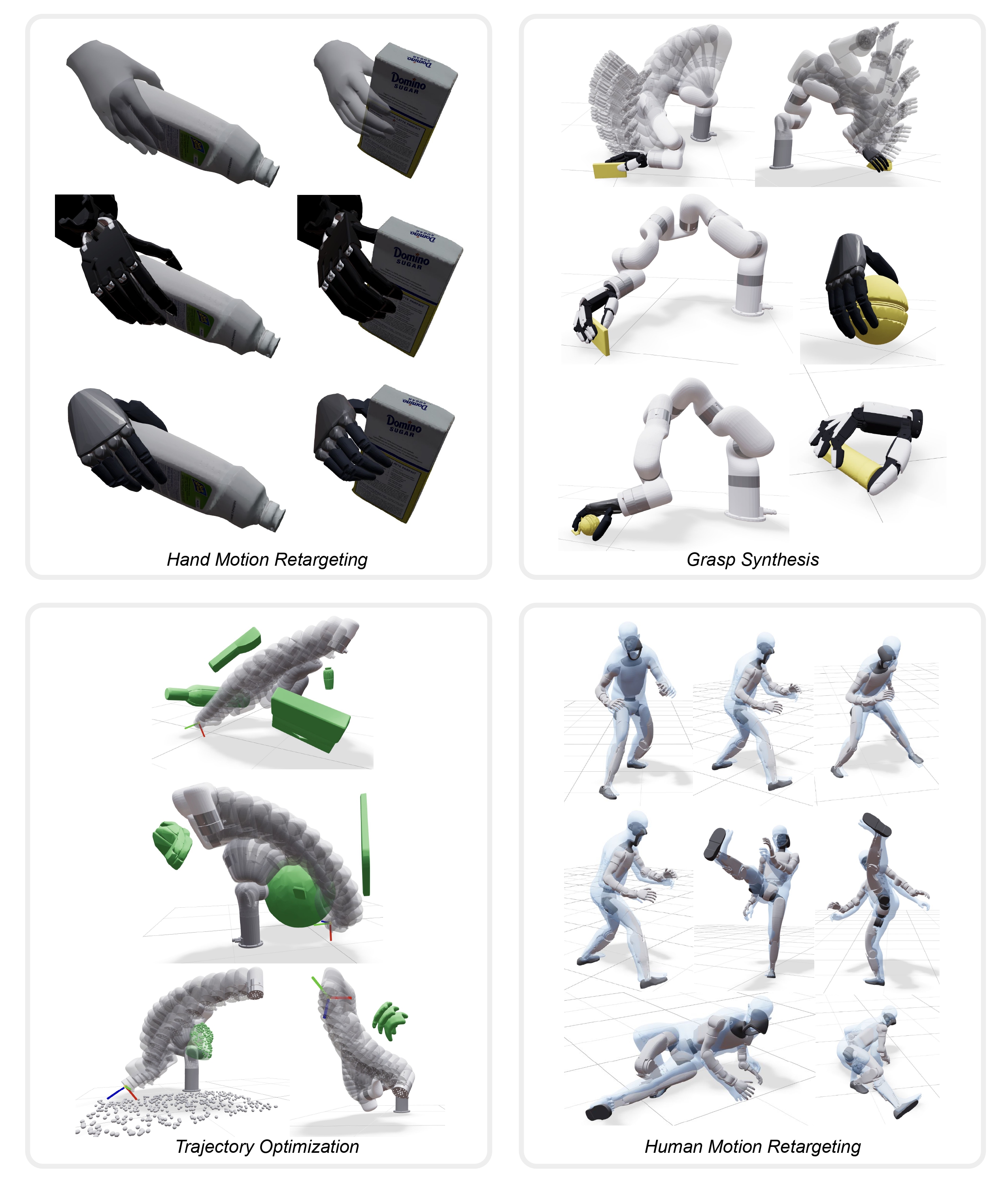
Figure 4 preserves the full montage for hand retargeting, grasp synthesis, trajectory optimization, and human retargeting. These examples illustrate behavior; the tables above supply the quantitative evidence.