Reading guide
This edition covers the complete 37-page paper and supplement, preserving ten figures, three tables with their symbol legends, all numbered equations, the dataset command and original project media. Read the architecture first, then sensor models and calibration. The evidence concerns open-loop measurements and selected perception pipelines; closed-loop robot-control gains are future work.
At a glance
VisionSIM separates scene rendering from sensor emulation, exposing physical measurement parameters for conventional, single-photon, event, time-of-flight, thermal and inertial sensors. It reproduces selected saturation, pileup, wrapping, refractory and thermal-history effects from common reference scenes. A commercial LiDAR twin and several small fidelity studies support this modeling approach. The released indoor instantiation has 100 scenes and 480,000 stereo ground-truth views; scripts regenerate sensor streams. It is not a broad cross-device or closed-loop validation.
1 Introduction
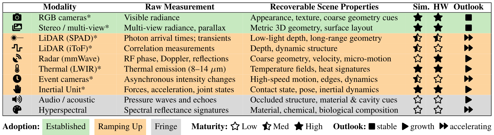
Ideal scene truth can conceal the sensor failures a robot actually encounters. VisionSIM makes raw measurement formation configurable, allowing candidate sensors to share scene geometry and trajectories. Existing physics/rendering engines remain the substrate; the contribution combines sensor breadth, parameter control and selected failure models. The taxonomy is the authors’ qualitative assessment of maturity/adoption, not a measured market survey.
Accessible table, original values and symbol meanings
| Modality | Raw Measurement | Recoverable Scene Properties | Sim. | HW | Outlook | |
|---|---|---|---|---|---|---|
| camera | RGB cameras* | Visible radiance | Appearance, texture, coarse geometry cues | high | high | stable |
| multi-view | Stereo / multi-view* | Multi-view radiance, parallax | Metric 3D geometry, surface layout | high | high | stable |
| ✹— | LiDAR (SPAD)* | Photon arrival times; transients | Low-light depth, long-range geometry | medium | medium | accelerating |
| waveform | LiDAR (iToF)* | Correlation measurements | Depth, dynamic structure | medium | low | accelerating |
| radar | Radar (mmWave) | RF phase, Doppler, reflections | Coarse geometry, velocity, micro-motion | low | high | growth |
| thermal | Thermal (LWIR)* | Thermal emission (8–14 m) | Temperature fields, heat signatures | high | high | growth |
| clock | Event cameras* | Asynchronous intensity changes | High-speed motion, edges, dynamics | medium | low | accelerating |
| hand | Inertial Unit* | Forces, acceleration, joint states | Contact state, pose, inertial dynamics | high | high | growth |
| audio | Audio / acoustic | Pressure waves and echoes | Occluded structure, material & cavity cues | low | low | growth |
| color | Hyperspectral | Spectral reflectance signatures | Material, chemical, biological composition | low | low | accelerating |
Adoption: Established Ramping Up Fringe Maturity: low Low medium Med high High Outlook: stable stable growth growth accelerating accelerating
2 Related Works
Task datasets, general-purpose simulation and specialist sensor emulators supply complementary pieces. VisionSIM combines shared rendered truth with modality-specific forward models, reusing earlier sensor/interpolation methods rather than replacing all of them. Thermal history and photon timing extend beyond adding generic image noise. Coverage comparisons alone do not prove uniform superiority over every specialist simulator.
3 Architecture Overview
The world layer renders clean radiance and dense truth; the sensor layer converts these into raw measurements. Replaying fixed truth avoids new rendering when sensor parameters change, although emulation still costs computation. Distributed Blender jobs, keyframe remapping and interpolation reduce rendering expense. Heat transport belongs in world simulation because thermal radiation depends on past energy exchange, not only current visible appearance.
Original mathematical definitions and modeling assumptions
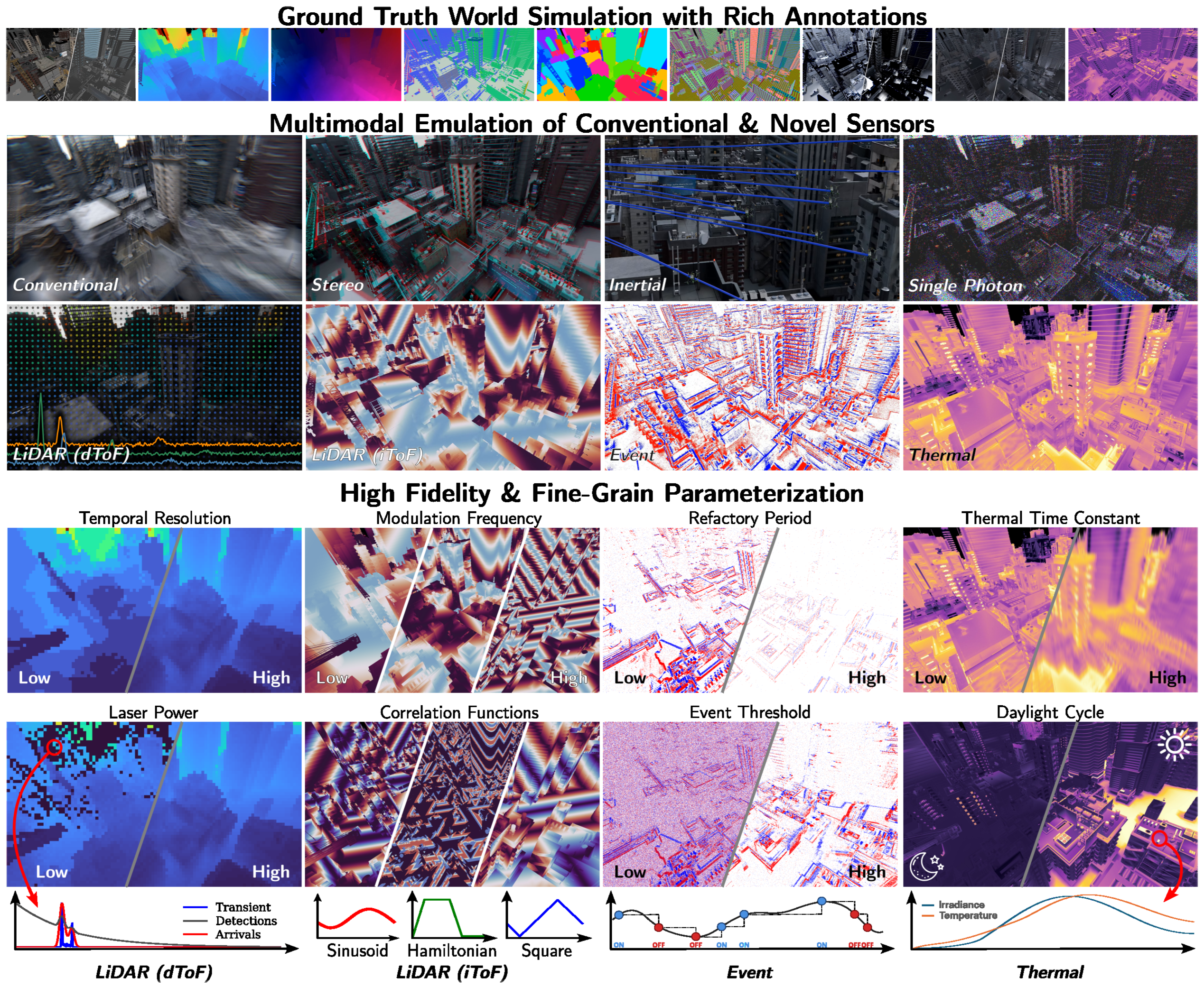
Sensor Emulation Layer. This layer ingests the noise-free, high-frame-rate data and transforms them into realistic sensor measurements. Rather than applying generic additive Gaussian noise to idealized outputs, it implements physically constrained, per-modality measurement models from which noise, distortions, and failure modes naturally emerge as physical consequences. The layer supports conventional and high-speed cameras, stereo and multi-camera rigs, passive single-photon cameras, single-photon (dToF) LiDAR, indirect time-of-flight (iToF) LiDAR, event cameras, thermal cameras, and inertial measurement units. Since it operates on shared reference frames, any subset can be co-simulated on identical scenes and trajectories. The resulting multi-modal measurements are saved in a compressed, sensor-aware format compatible with downstream learning frameworks [90, 8]; stochastic binary single-photon frames, in particular, are stored in a bit-packed manner that achieves lossless compression with on-the-fly random access (Appendix S.4).
4 Physically-Grounded Sensor Models and Failure Modes
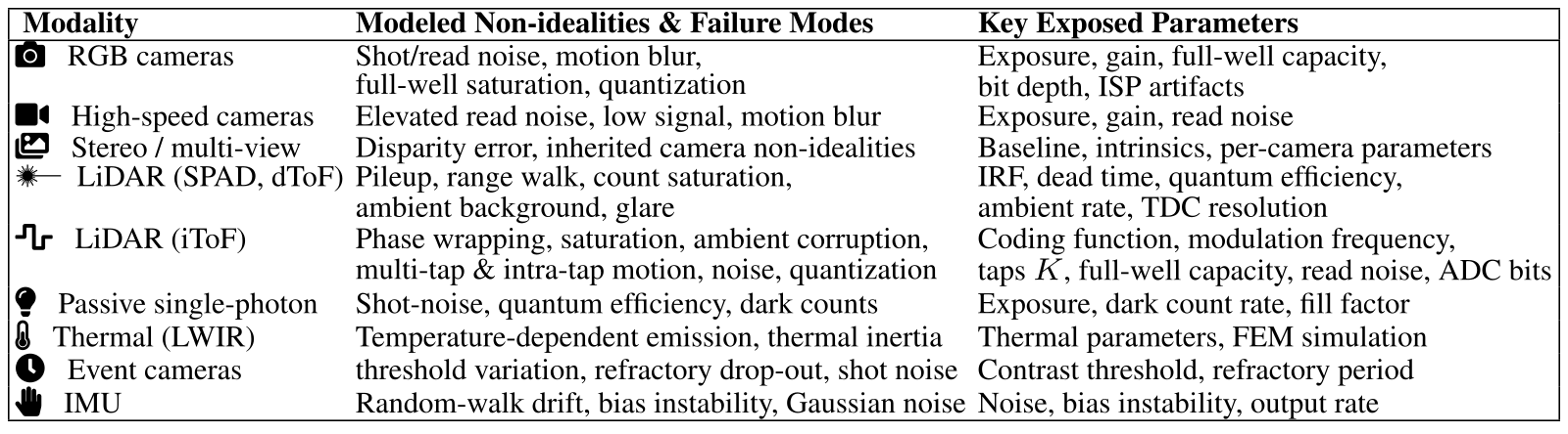
Three detailed models illustrate the approach: active photon timing, modulated-light correlation and thermal emission/detector inertia. Their failure modes follow specific approximations and available reference data. Table 2 lists modeled effects and exposed parameters; it does not claim every real optical/electronic effect is present.
Accessible table, original values and symbol meanings
| Modality | Modeled Non-idealities & Failure Modes | Key Exposed Parameters |
|---|---|---|
| camera RGB cameras |
Shot/read noise, motion blur,
full-well saturation, quantization |
Exposure, gain, full-well capacity,
bit depth, ISP artifacts |
| video High-speed cameras | Elevated read noise, low signal, motion blur | Exposure, gain, read noise |
| multi-view Stereo / multi-view | Disparity error, inherited camera non-idealities | Baseline, intrinsics, per-camera parameters |
| ✹— LiDAR (SPAD, dToF) |
Pileup, range walk, count saturation,
ambient background, glare |
IRF, dead time, quantum efficiency,
ambient rate, TDC resolution |
| waveform LiDAR (iToF) | Phase wrapping, saturation, ambient corruption, multi-tap & intra-tap motion, noise, quantization |
Coding function, modulation frequency,
taps , full-well capacity, read noise, ADC bits |
| lighting Passive single-photon | Shot-noise, quantum efficiency, dark counts | Exposure, dark count rate, fill factor |
| thermal Thermal (LWIR) | Temperature-dependent emission, thermal inertia | Thermal parameters, FEM simulation |
| clock Event cameras | threshold variation, refractory drop-out, shot noise | Contrast threshold, refractory period |
| hand IMU | Random-walk drift, bias instability, Gaussian noise | Noise, bias instability, output rate |
4.1 Single-Photon (dToF) LiDAR
A per-pixel field-of-view mask aggregates albedo/depth contributions into a temporal response; convolution with an impulse response and ambient photon rate precedes stochastic arrival/detection modeling. Non-paralyzable dead time discards detections during recovery and can bias high-flux histograms toward earlier ranges. Spatial optical effects use the mask/PSF abstraction. SPAD crosstalk is explicitly not yet modeled, and full volumetric transport is outside this abstraction.
Original mathematical definitions and modeling assumptions
Commercial solid-state LiDAR is rapidly adopting single-photon avalanche diode (SPAD) arrays [38, 91] to capture photon-arrival histograms for depth estimation. VisionSIM physically models the histogram acquisition pipeline. For each pixel, the discrete scene response at bin index aggregates the radiometric contributions of scene points within a field-of-view mask as

Original selectable equation (1)
Equation 1
| (1) |
Original mathematical definitions and modeling assumptions
where is the temporal bin width, is albedo, the inverse-square falloff, the mask weight, and the quantum efficiency. The spatially-resolved mask models common optical effects like vignetting and blooming from retroreflective returns (Section 5). SPAD crosstalk is not yet modeled; it can be added as a per-pixel spatial kernel applied to the transient, which would capture optical and electrical coupling between neighbouring detectors. The total photon-arrival rate is then modeled as , where is a constant background rate, and is the system’s impulse response function (IRF), a calibrated or parametric laser pulse. Finally, incident photon counts are drawn from an inhomogeneous Poisson process governed by .
4.2 Indirect Time-of-Flight (iToF) LiDAR
An iToF sensor integrates phase-shifted correlation taps before decoding depth. Modulation frequency limits unambiguous range; clipping, ambient photons, read noise, quantization and sequential/intra-tap motion corrupt the taps. Figures retain each isolated failure example. Multiple taps acquired at different times can disagree on moving boundaries; these are measurement artifacts rather than changes to geometric ground truth.
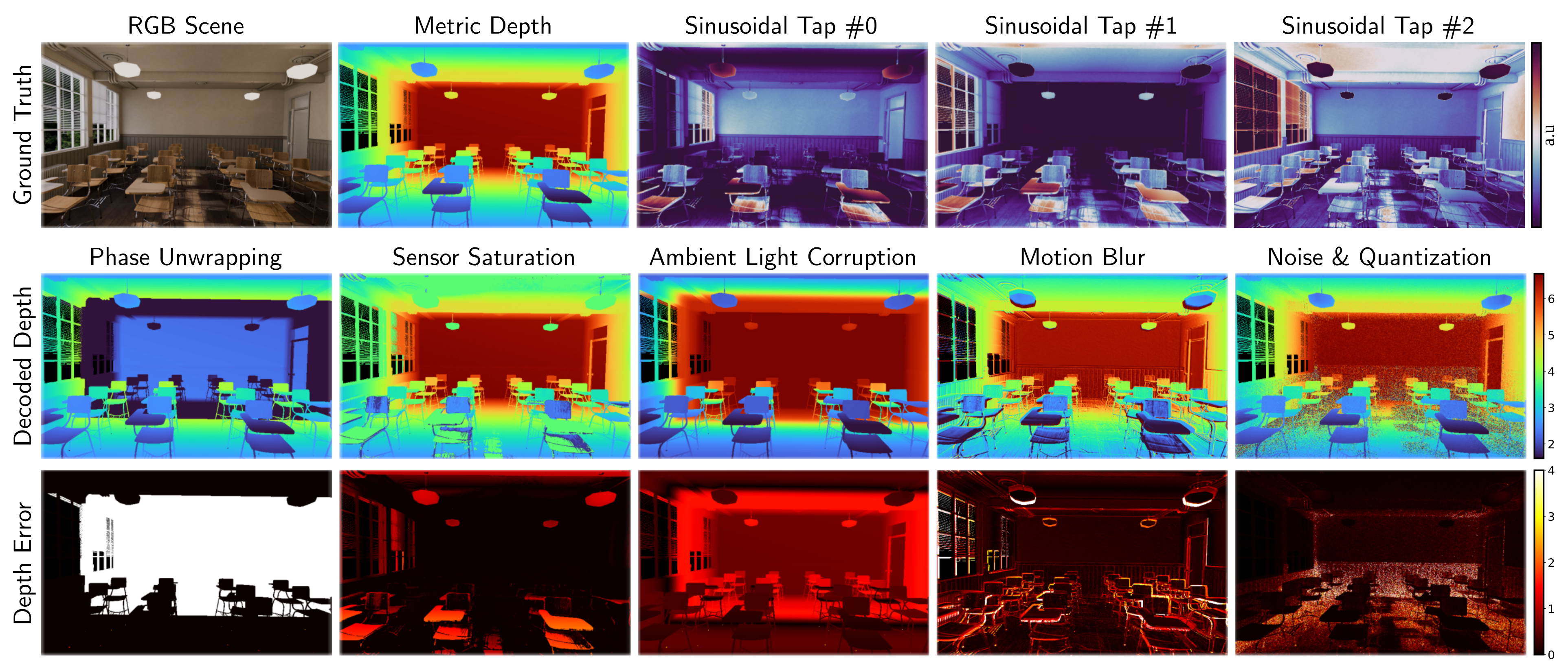
Original mathematical definitions and modeling assumptions
Indirect, or continuous-wave, time-of-flight cameras are similarly widespread, shipping in consumer and industrial depth sensors from major manufacturers [39, 86]. Rather than timing individual photons, they recover depth from the phase of amplitude-modulated light [48]: the scene is illuminated with a periodically modulated source, and the sensor correlates the returning light against phase-shifted demodulation functions, producing correlation taps from which depth is decoded. Following the continuous-wave image-formation model [32], the -th measured tap at a pixel is:

Original selectable equation (2)
Equation 2
| (2) |
Original mathematical definitions and modeling assumptions
where is the scene depth, the normalized correlation function for tap (set by the coding scheme), includes albedo and distance-squared falloff, is the ambient component, is shot and read noise, and models sensing non-idealities (e.g., ADC quantization, saturation).
Original mathematical definitions and modeling assumptions
Equation 2 captures physical failure modes explicitly (Figure 2): (i) Phase wrapping: depth wraps beyond the unambiguous range, , set by the modulation frequency , rendering distant objects close; (ii) Saturation: measurements clip when signal exceeds full-well capacity; (iii) Ambient corruption: large reduces modulation contrast, corrupting depth particularly for distant, dimly-lit points; (iv) Motion artifacts: intra- and inter-tap motion (for sequential taps) cause spatial tearing and boundary ghosting, which we model by integrating temporally offset interpolated frames; (v) Noise & quantization: and cause high-frequency depth errors and banding.
4.3 Thermal Cameras
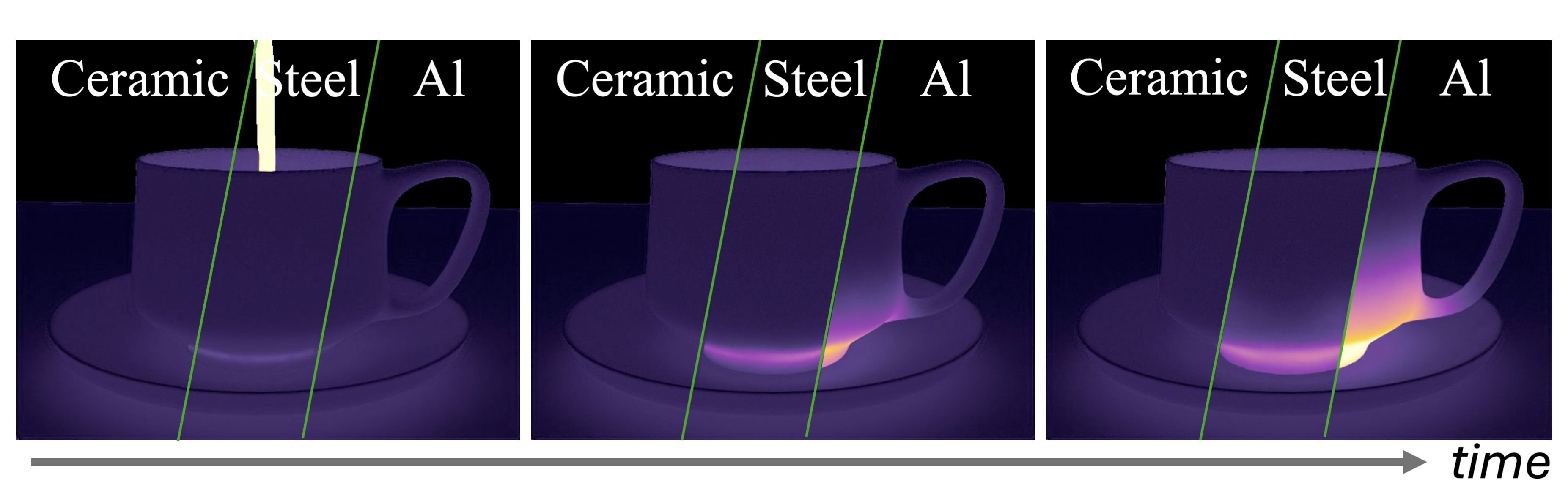
Thermal image formation requires a temperature field with material- and history-dependent dynamics. The world heat solver supplies that field; graybody emission/reflection and microbolometer lag then form the image. The cup sequence illustrates differing diffusivities over four seconds. Surface emissivity, heat-transfer assumptions and omitted detector noise limit fidelity beyond that example.
5 Case Studies: Design and Analysis of Robot Perception Systems
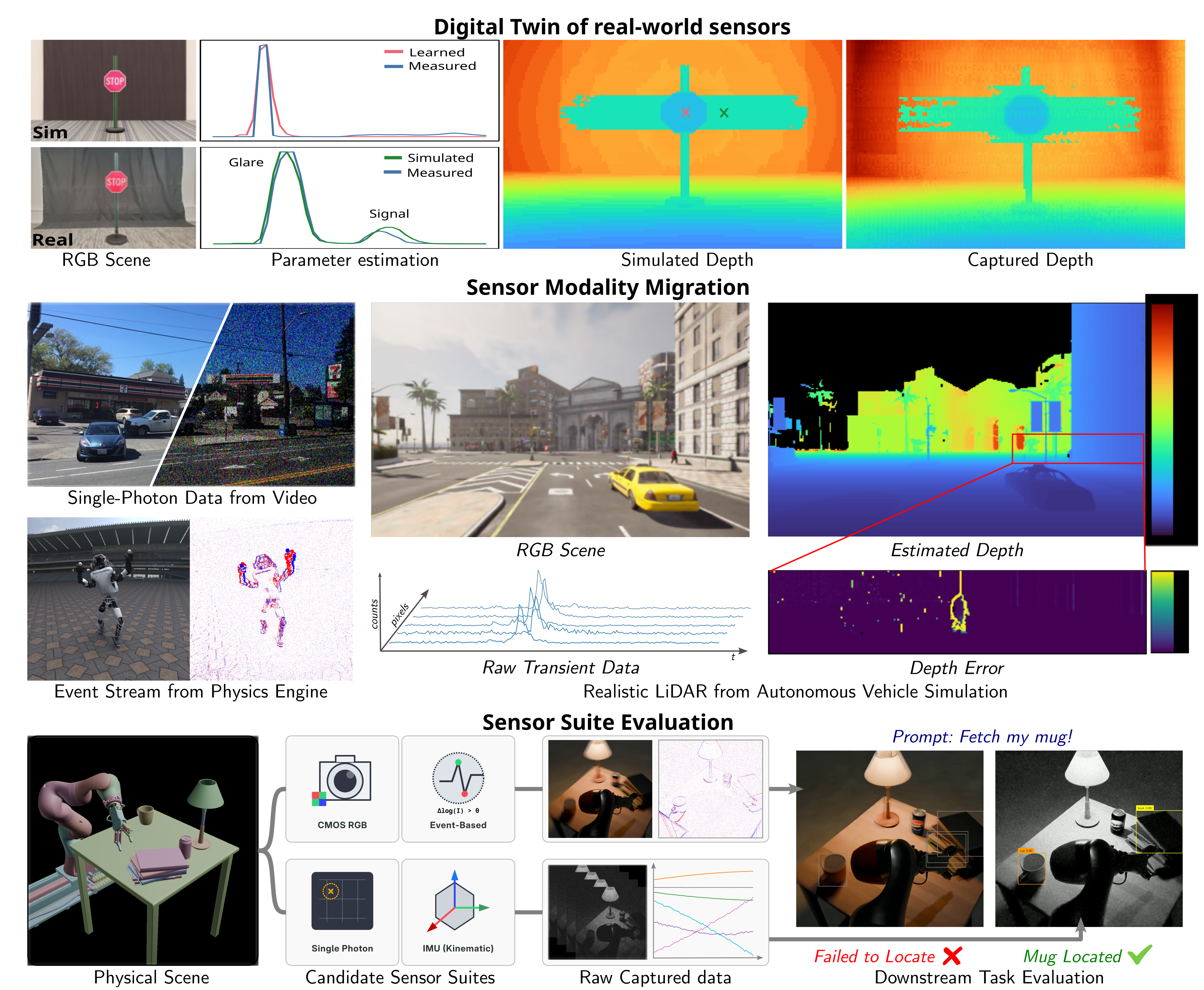
Three proof-of-concept applications use the shared measurement interface: a calibrated LiDAR twin, migration of existing data to additional modalities, and one low-light sensor-suite comparison. All are open-loop. The suite comparison includes reconstruction and detection networks used zero-shot, so its single example evaluates the whole pipeline rather than isolating a sensor’s inherent advantage.
Original mathematical definitions and modeling assumptions
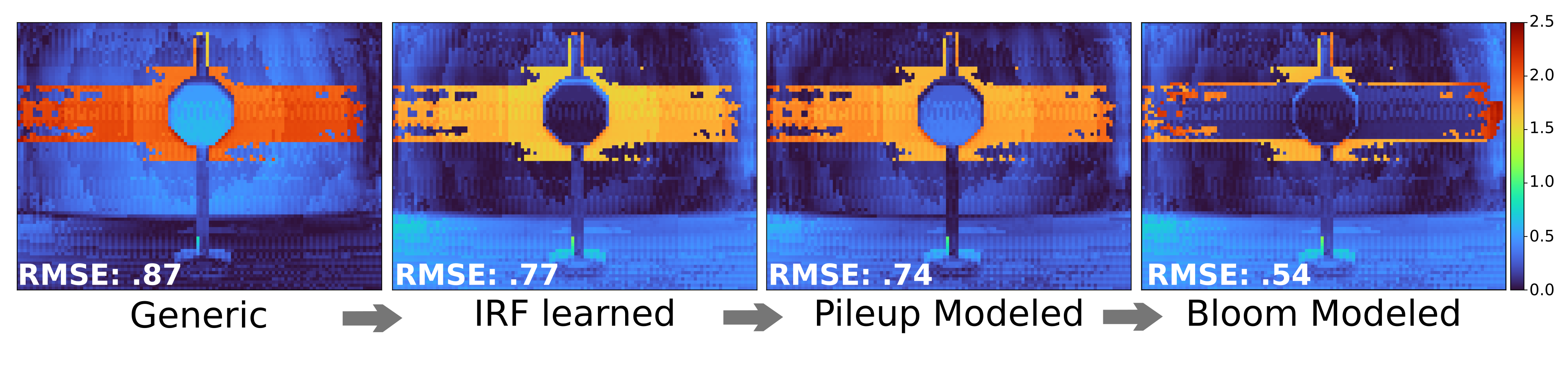
We build a digital twin of a commercial single-photon LiDAR (Adaps Photonics ADS6311 [1]; details in Appendix S.6). Because VisionSIM’s dToF model is differentiable, we recover the device’s parameters directly from real captures via gradient-based fitting of a measurement-matching loss, which we demonstrate with the sensor’s impulse response function (IRF). We validate the twin on a scene captured in the lab and modeled in Blender (Figure 4, top), chosen because it exercises two failure modes at once. The retroreflective sign produces an intense return that saturates the detector; the recovered IRF and dead time reproduce the resulting pileup and range-walk error. That same intense return induces glare through internal multipath between the sensor optics and the detector array, which the spatially-varying PSF captures, reproducing the characteristic point-cloud ghosting. The resulting reconstructed depth closely tracks the device’s measured depth. Faithfully modeling the IRF, pileup, and glare lowers the RMSE of the digital twin by meters.
Original mathematical definitions and modeling assumptions
Migrating existing datasets to new sensing modalities. The decoupled architecture also enables migrating existing datasets to modalities they were never captured with, by bypassing world simulation and feeding pre-existing data directly to the sensor emulation layer. We show three examples (Figure 4, middle): emulating a passive single-photon camera from the XVFI high-speed video dataset [84]; generating an event stream from a Genesis render of a dancing humanoid [3, 100]; and producing raw single-photon LiDAR transients from a CARLA driving sequence [20]. Uplifting a conventional autonomous-driving dataset into time-resolved single-photon measurements lets sensor-specific failure modes be exposed: here, the pedestrian might not be detected at the sensor level as their lateral motion induces motion blur within the transient histograms, causing depth errors in excess of meters. This lets researchers obtain data for emerging sensors by reusing existing assets, rather than recapturing scenes with specialized and often unavailable hardware. Dataset migration is bounded by what the source data contains: the frame rate caps the temporal resolution of the emulated sensor, and each modality needs its own annotations, so a dataset without depth cannot be uplifted to iToF or dToF.
Original mathematical definitions and modeling assumptions
Evaluating & benchmarking sensor suites. Sensor emulation decoupling enables a single rendered scene to be replayed through many sensor configurations at no additional rendering cost, allowing comparisons of candidate suites before any hardware is built. We demonstrate this through a robot perception case study, where a system architect selects between two sensor suites for low-light, dynamic environments: a conventional camera paired with an event camera, or a passive single-photon camera and IMU. Both are emulated on identical high-speed trajectories; each suite’s raw measurements are reconstructed into image-like representations using existing methods [88, 53], and passed to an off-the-shelf detection and tracking model [73] to compare downstream task performance (Figure 4, bottom). Detection fails in the first case, while the second sensor suite yields confidence. Both reconstruction models and the detector are used zero-shot, so the result characterizes the full pipeline rather than the sensor suite alone; retraining on raw measurements would remove the reconstruction bias. Sweeping sensor parameters (exposure, event threshold, fill factor, etc.) within the same framework lets the architect map the trade-off across operating regimes, a comparison that is prohibitively expensive to perform with real hardware.
6 Sim-to-Real Validation
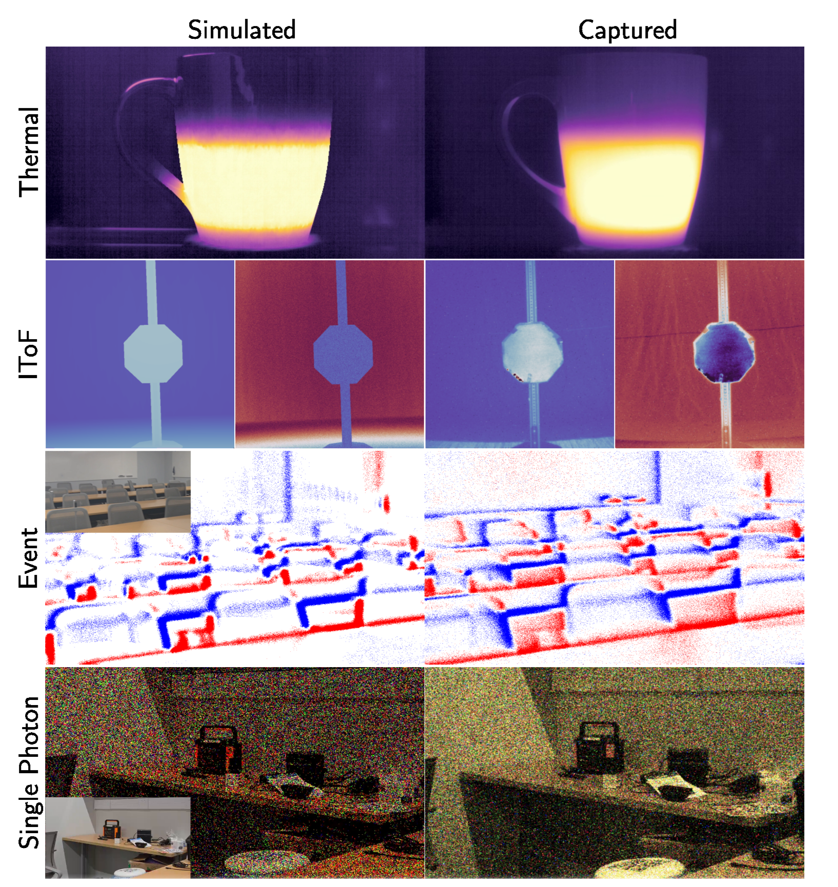
Small modality-specific checks compare simulated and captured data: thermal heating error is 7.6% of the observed dynamic range; iToF phase error is 0.13 rad; positive/negative event counts differ by 1.5%/5.8%; photon detection statistics are 0.221 versus 0.229. These aggregate similarities do not establish matching event timing, spatial errors or broad device coverage. The stated conversion of 0.13 rad at 40 MHz to 5.3 cm is inconsistent with the usual two-way phase formula, which gives about 7.8 cm. End-to-end scene twins and emulation from co-located RGB are different protocols; unknown source-camera photometry limits the latter.
Original mathematical definitions and modeling assumptions
For a mug filling with hot tea, the simulated heating profile tracks a real-world capture from a FLIR Boson to within a mean absolute error of of the real mug’s heating dynamic range over the 4 seconds following the fill. Against a real capture of a STOP sign taken with a Chronoptics iToF camera, our emulated iToF sensor achieves a mean phase error of radians across a range. At a 40 MHz modulation frequency, this translates to a mean depth error of about cm. Event counts emulated on RGB video of an auditorium differ from a real recording taken with a Prophesee EVK4 sensor by for positive events and for negative events. The photon detection statistics of our emulated Pi-Imaging SPAD sensor, likewise driven by RGB video, reach against a measured .
7 The VisionSIM Multi-Modal Sensor Dataset
One hundred indoor scenes each have a 24-second stereo trajectory at 100 fps and 1000×1000 HDR, giving 100×24×100×2 = 480,000 views. Shared truth drives 16 kHz photon and 4 kHz event emulation, a 25 fps conventional camera and other modalities. Interpolated temporal sampling is not independently rendered truth at those higher rates. The release supplies ground truth, assets/configurations and regeneration scripts rather than claiming every large raw sensor stream is bundled.
Original mathematical definitions and modeling assumptions
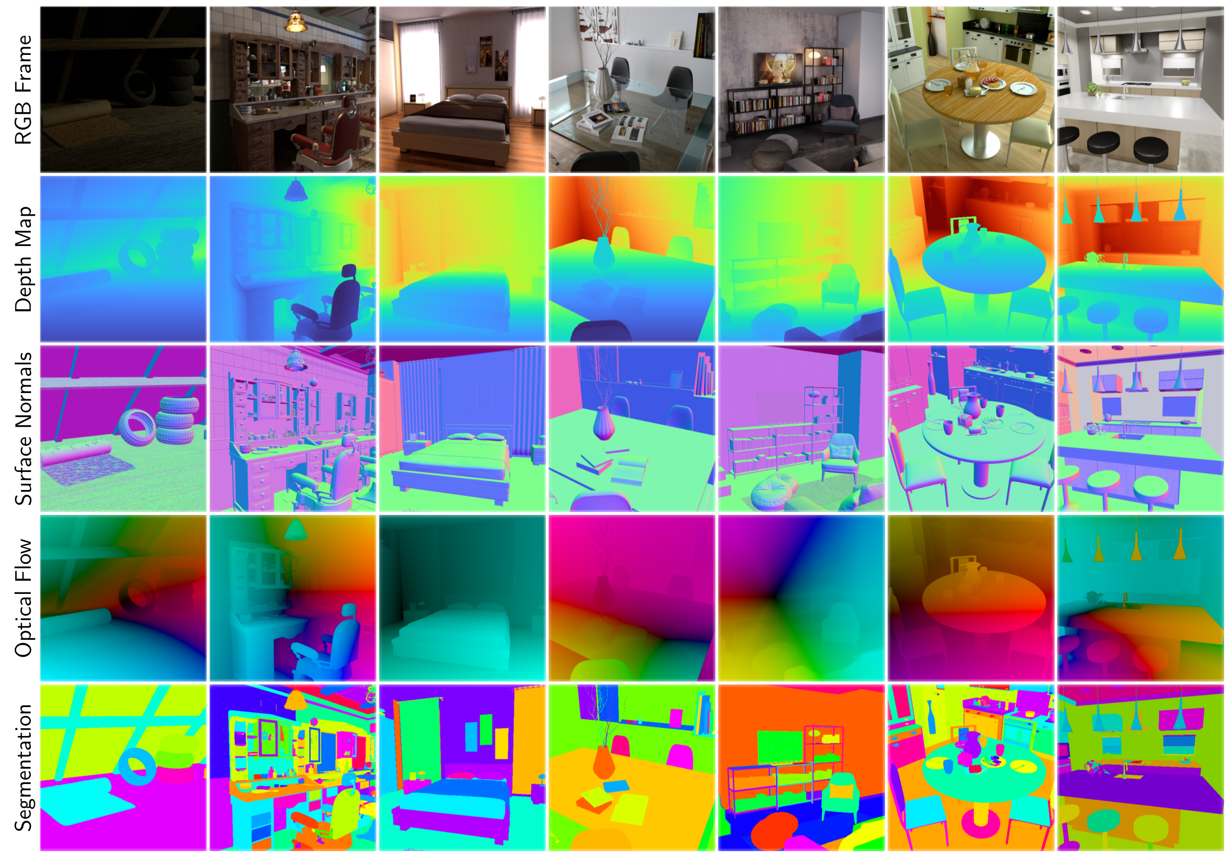
An indoor instantiation. We curate unique indoor scenes spanning offices, kitchens, bathrooms, etc., each with a predefined -second camera trajectory. Each scene is rendered at fps in HDR at as a stereo pair, with ground-truth poses, intrinsics, depth, surface normals, optical and scene flow, segmentation, temperature, and direct/indirect illumination components, yielding synchronized ground-truth views. From these, we emulate the full sensor suite: a single-photon camera at kHz (via interpolation), a kHz event camera (), a fps conventional camera, dToF and iToF LiDAR, a thermal sensor, an IMU at Hz, and a stereo rig, using representative noise parameters drawn from the literature [21, 65, 51, 35, 29, 6, 49, 56, 31, 32, 37].
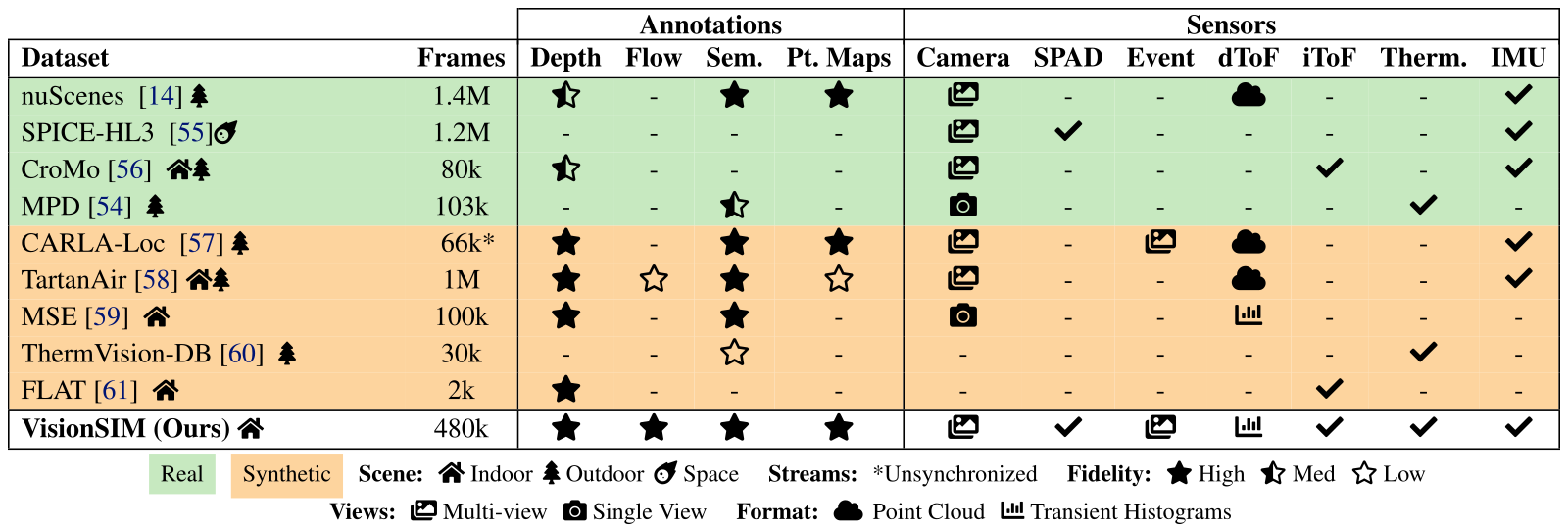
Accessible table, original values and symbol meanings
| Annotations | Sensors | |||||||||||
|---|---|---|---|---|---|---|---|---|---|---|---|---|
| Dataset | Frames | Depth | Flow | Sem. | Pt. Maps | Camera | SPAD | Event | dToF | iToF | Therm. | IMU |
| nuScenes [10] outdoor | 1.4M | medium | - | high | high | multi-view | - | - | point cloud | - | - | yes |
| SPICE-HL3 [74] space | 1.2M | - | - | - | - | multi-view | yes | - | - | - | - | yes |
| CroMo [97] indoor outdoor | 80k | medium | - | - | - | multi-view | - | - | - | yes | - | yes |
| MPD [37] outdoor | 103k | - | - | medium | - | single view | - | - | - | - | yes | - |
| CARLA-Loc [33] outdoor | 66k* | high | - | high | high | multi-view | - | multi-view | point cloud | - | - | yes |
| TartanAir [99] indoor outdoor | 1M | high | low | high | low | multi-view | - | - | point cloud | - | - | yes |
| MSE [47] indoor | 100k | high | - | high | - | single view | - | - | transient histograms | - | - | - |
| ThermVision-DB [23] outdoor | 30k | - | - | low | - | - | - | - | - | - | yes | - |
| FLAT [30] indoor | 2k | high | - | - | - | - | - | - | - | yes | - | - |
| VisionSIM (Ours) indoor | 480k | high | high | high | high | multi-view | yes | multi-view | transient histograms | yes | yes | yes |
Real Synthetic Scene:
indoor Indoor
outdoor Outdoor
space Space Streams:
*Unsynchronized Fidelity:
high High
medium Med
low Low
Views:
multi-view Multi-view
single view Single View Format:
point cloud Point Cloud
transient histograms Transient Histograms
8 Limitations and Outlook
Validation uses one commercial LiDAR and a few scenes/measurements; no physical or simulated perception–control loop is closed. Indoor coverage, simplified optical transport and interpolation constrain transfer. Radar, wave effects, weather, real-time closed-loop simulation and broader calibrated device presets remain outlook items. Fine-grained parameters enable investigation but do not themselves certify sim-to-real reliability.
Acknowledgments
The authors acknowledge the listed funding programs, data-collection help and discussions about thermal simulation.
Original sensor and rendering demonstrations
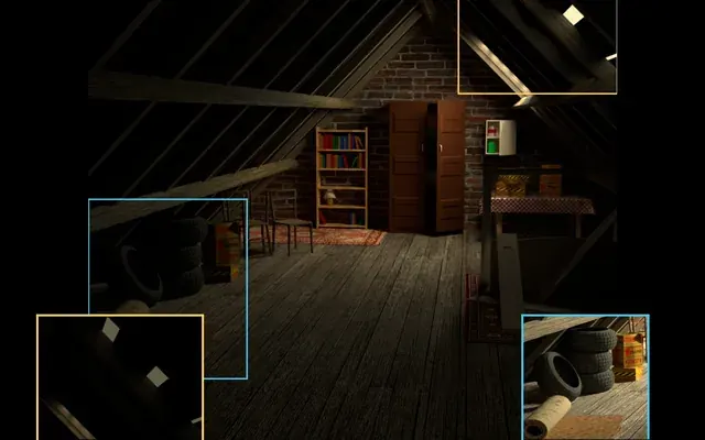
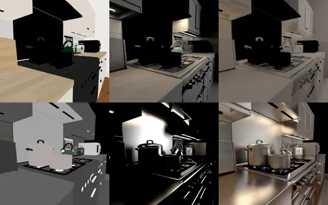
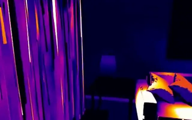
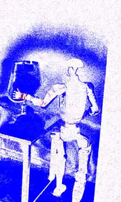
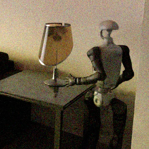
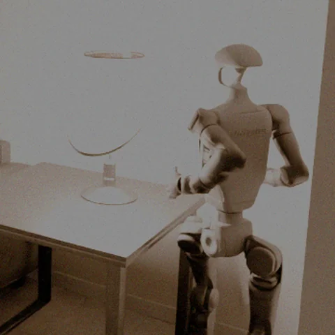
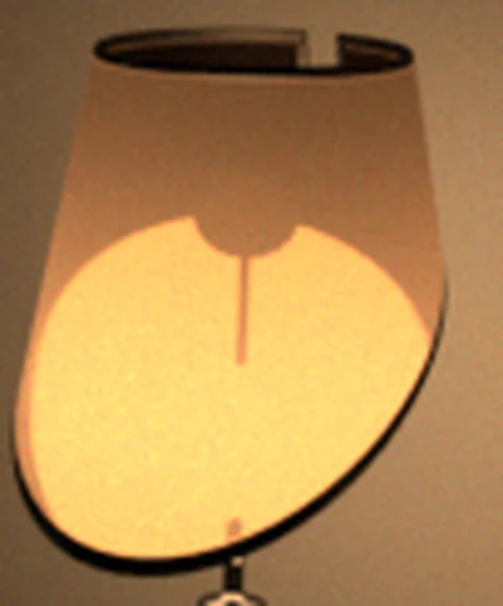
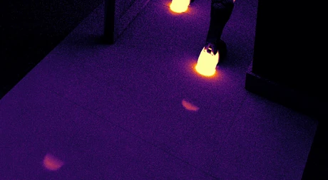
The original project page provides sensor, shared-scene-layer and rendering examples. All 30 published movies, their original posters and additional example stills are retained byte-for-byte. These explanatory clips add no independent robot trials. Source code and documentation remain linked through the primary repository and documentation; large scene/dataset downloads remain external.
S.1 Architecture
The supplement explains how the world/sensor layers can be used together or independently through a command-line interface and library. Migrated video can bypass rendering, but must supply the information each sensor requires. Matching output timestamps cannot recover missing physical inputs such as depth or a calibrated radiometric response.
S.2 World simulation
Blender provides clean frames and annotations, while a higher-level API coordinates rendering and sampling. The approach targets reuse of authored scenes and high-rate data generation. Expensive photorealistic rendering is distributed or temporally interpolated; neither makes all scene dynamics or arbitrary high-rate measurements exact.
S.2.1 Streamlined API
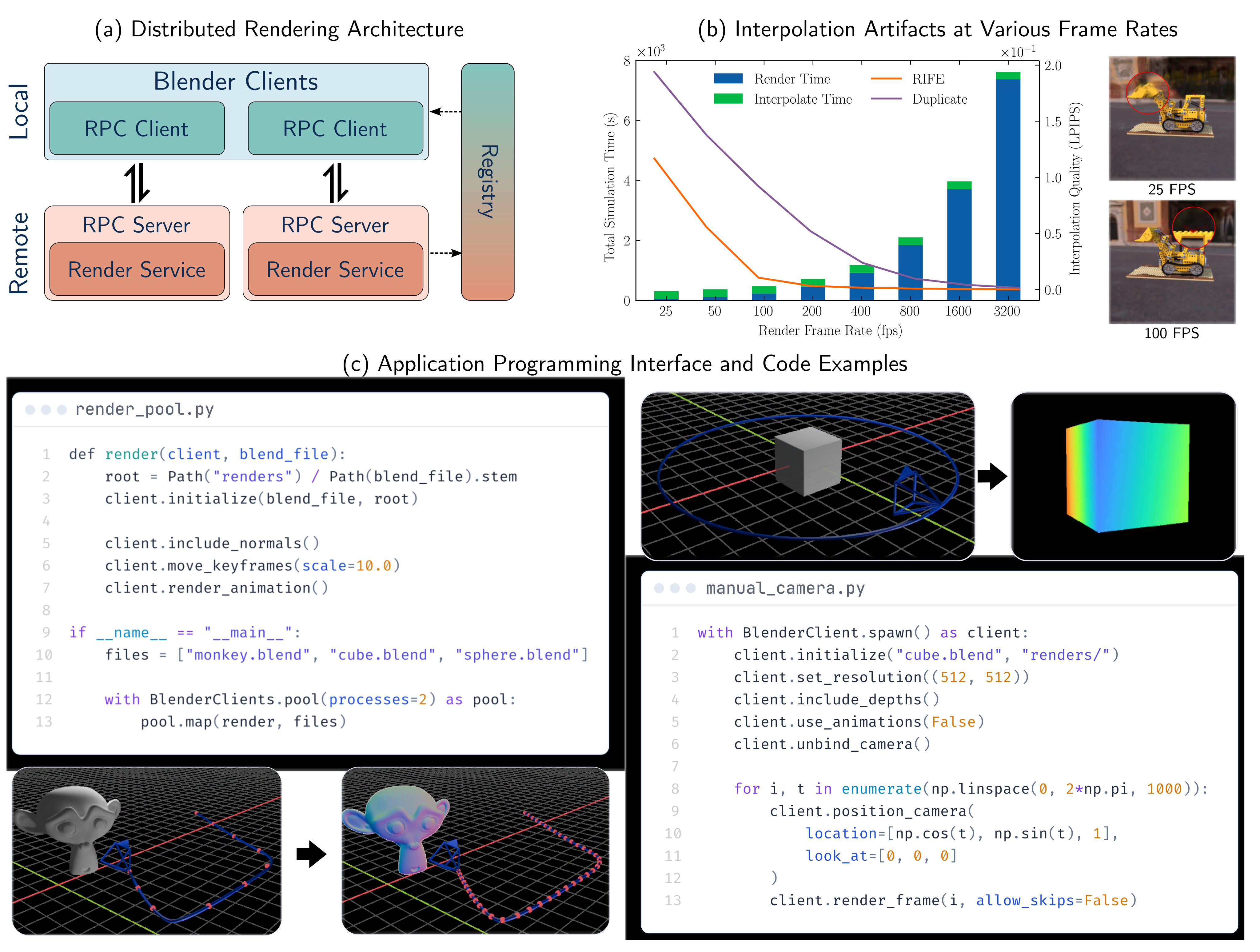
The simplified API drives Blender’s internal bpy functionality through a server and adds requested annotation passes. It keeps authored scene settings unless changed explicitly. Inputs must still be valid renderable blend files; the interface does not repair arbitrary broken assets. Figure S1 preserves both complete code examples and their rendered results.
S.2.2 Distributed rendering
RPC render services announce themselves through a UDP registry, enabling heterogeneous workers and multiple jobs per host. Larger generation uses Docker jobs on HTCondor. This improves orchestration and utilization; no universal throughput claim follows across hardware, scene complexity or cluster allocation. The paper’s runtime examples use a specific RTX 3080 job.
S.2.3 Keyframe remapping
Remapping animation keyframes dilates authored time so more samples can be obtained without requiring assets designed at extreme frame rates. The method resamples existing splines/baked motion. It does not create physically correct unseen high-frequency behavior absent from the authored/baked scene.
S.2.4 Physics engine
Blender/Bullet can bake rigid, soft-body, cloth and fluid effects into reusable motion, then remap those keyframes. Baking and temporal resampling are distinct from rerunning physics with a more accurate collision/time-step model. The contribution is compatibility and reuse within the rendering pipeline.
S.2.5 Heat Transport Simulation
Thermal rendering starts from temperature evolution, driven by absorbed visible irradiance and thermal exchange. The supplement gives the full light-to-heat and discrete solver formulation. Ambient/material parameters and initial/boundary conditions are substantive inputs even when light-driven heat sources are obtained automatically from rendering.
Original mathematical definitions and modeling assumptions
Several sensor modalities of interest—most notably long-wave infrared (LWIR, –) thermal cameras—respond not to the instantaneous radiance leaving a surface, but to the long-wave radiation it emits as a consequence of its temperature, and that temperature is the accumulated result of every watt of power the surface has absorbed over the preceding seconds to hours. Synthesizing a thermal image therefore requires synthesizing a plausible temperature field first, which the sensor emulation layer (Sec. S.5.4) then renders into a measurement. To support these modalities, VisionSIM integrates a fast, GPU-accelerated heat-transport solver directly into the world simulation layer, reusing the same Blender asset-authoring and rendering pipeline described above so that the temperature field is always consistent with the exact lighting the scene was authored with. This section develops the forward model in two stages: how absorbed visible light becomes a heat source (Sec. S.2.5.1), and how the resulting heat-transport PDE is discretized and solved (Sec. S.2.5.2).
S.2.5.1 Visible Light to Thermal Heat Source
For opaque Lambertian surfaces, reflected visible intensity and absorbed irradiance are complementary under the chosen albedo/absorptivity model. Diffuse irradiance passes supply spatial heat inputs, which are mapped to mesh vertices. Visible albedo is not a universally calibrated broadband absorptivity, especially for glossy or spectrally complex materials. The original equations and assumptions remain selectable.
Original mathematical definitions and modeling assumptions
The bridge between the visible-band light transport that VisionSIM already simulates and the thermal domain is energy conservation at an opaque surface. The pixel value an ordinary camera records is the fraction of incident light reflected toward it; since an opaque surface transmits nothing, the remaining energy is absorbed, converted to heat, and subsequently redistributed by conduction, convection, and re-radiation, governed by the heat-transport equation [63]. Reflection and absorption are thus complementary [70], and the same path-traced irradiance the renderer evaluates to form the visible image also determines the heat deposited at each surface. Making this precise for a Lambertian scene point , let denote the incident visible-band radiant flux density () arriving at under the scene’s lighting. A camera focused at measures only the reflected portion, giving the visible image intensity

Original selectable equation (S1)
Equation S1
| (S1) |
Original mathematical definitions and modeling assumptions
where is the pixel imaging and is the surface albedo. The complementary absorbed power per unit area—the quantity that drives the heat equation—is the remaining fraction,

Original selectable equation (S2)
Equation S2
| (S2) |
Original mathematical definitions and modeling assumptions
which enters the thermal problem as a Neumann boundary source (Sec. S.2.5.2). The broadband absorptivity generalizes the ideal Lambertian factor to account for surface finish and angular reflectance, and reduces to it when the user ties absorption directly to the visible albedo.
Original mathematical definitions and modeling assumptions
The decisive modeling choice is that we obtain directly from the renderer rather than asking the user to specify a heat flux by hand, as classical FEM packages (ANSYS [2], COMSOL [15], OpenFOAM [67]) require. Concretely, we read from the renderer’s diffuse irradiance passes—the direct and indirect diffuse light transport that already produces the matte component of the RGB image, including indirect bounces, environment lighting, sky and sun, and animated emitters—baked into a per-texel irradiance map at each timestep and resampled to mesh vertices by barycentric interpolation. The practical consequence is that the temperature field is always consistent with the exact lighting the scene was authored with: moving the sun to a different time of day moves the heat input, adding an emitter adds a heat source, and turning off a lamp removes its thermal contribution—all without the user authoring any thermal boundary condition.
S.2.5.2 Finite Element Heat Transport Simulation
A heat equation with boundary exchange is discretized over robust mesh/point operators and advanced implicitly. The implementation aims to tolerate imperfect graphics assets while reusing a constant matrix when radiation is linearized around fixed ambient temperature. This is a practical approximation, not a convergence or accuracy guarantee for every non-manifold asset and material field.
Governing PDE.
Temperature change depends on density, heat capacity and conductivity, with diffusivity controlling transient spread. The presented experiments inject energy through boundary conditions rather than a nonzero volumetric source. Material values and units matter; the illustrative diffusivity ratios are approximate.
Original mathematical definitions and modeling assumptions
We model heat transport in a solid domain (following [63]) with boundary , exchanging energy with an ambient at temperature through convection and radiation while absorbing externally driven irradiance on . The temperature field satisfies the inhomogeneous heat equation

Original selectable equation (S3)
Equation S3
| (S3) |
Original mathematical definitions and modeling assumptions
where , , and are the spatially varying density, specific heat capacity, and thermal conductivity, and is a volumetric source. We take and inject all energy through the boundary. The transient response is governed by the thermal diffusivity , which is the natural parameter to reason about: aluminum () diffuses heat roughly faster than glass (), and it is this ratio rather than the conductivity alone that distinguishes their thermal appearance over the timescale of a video.
Boundary conditions.
Boundary heat loss combines convection and radiation to ambient; selected contact/heater regions can instead impose Dirichlet temperatures. An initial temperature field is required. These conditions model specified surroundings and contacts rather than discovering unknown real heat transfer automatically.
Original mathematical definitions and modeling assumptions
A surface has no thickness and hence zero mass, so it cannot store energy and any heat entering it must exit on the other side. On this balance is the Robin-type condition

Original selectable equation (S4)
Equation S4
| (S4) |
Original mathematical definitions and modeling assumptions
where is the outward unit normal, is the Stefan–Boltzmann constant, is the LWIR emissivity, and is the convective heat-transfer coefficient. The left-hand side is the conductive flux through the surface given by Fourier’s law; the right-hand side is the flux lost to radiation and convection. Surfaces with externally imposed temperatures (a poured hot liquid, a thermostatic heater, a contact patch) are instead handled with Dirichlet conditions on user-tagged sub-regions , and the field is initialized from a per-vertex attribute that defaults to .
Combined heat equation.
The combined expression folds boundary losses and absorbed light into local energy balance. Equation S5 prints area factors on radiation/convection but not on q_abs, which the text defines as power per area; its dimensional convention therefore needs clarification. Equation S7 later applies the boundary area matrix. Both published expressions are retained without asserting an implementation bug.
Original mathematical definitions and modeling assumptions
Following [63], we fold the boundary condition directly into the energy balance of a finite element exposed to the surface with area . Adding the absorbed irradiance as an external input gives a single combined equation,

Original selectable equation (S5)
Equation S5
| (S5) |
Original mathematical definitions and modeling assumptions
where is the Laplace–Beltrami operator, is the input power per unit area () absorbed by the object on the boundary in the visible spectrum and is an indicator function which is 1 if the infinitesimal volume is on the surface and 0 otherwise.
Linearized radiation.
Linearizing quartic radiation about fixed ambient temperature permits matrix reuse for modest temperature differences. Large temperature excursions can require relinearization and repeated assembly. Stable time integration does not eliminate the physical error of that linearized radiation model.

Original selectable equation (S6)
Equation S6
| (S6) |
Original mathematical definitions and modeling assumptions
Crucially, this folds radiation into a constant boundary stiffness term that references only the fixed rather than the evolving solution, so the system matrix can be assembled once and reused across the animation, with only the lighting-dependent right-hand side reassembled per frame. For high-temperature targets (welding, furnace interiors etc.) the radiation term can instead be re-linearized about the current solution each step, at the cost of per-frame matrix reassembly.
Spatial discretization.
Lumped mass and area matrices integrate interior and boundary terms; an intrinsically mollified cotangent operator tolerates poor meshes. Spatially varying material coefficients and the printed Laplacian sign require a consistent discrete convention. Robustness to degenerate geometry does not make discretization error independent of resolution or guarantee the accuracy of an arbitrary graphics asset.
Original mathematical definitions and modeling assumptions
We represent the temperature as a piecewise-linear field over the discrete domain, , with the nodal basis functions, and discretize into finite elements with vertices. The discrete Laplace–Beltrami operator is , where is the cotangent Laplacian and the lumped vertex mass matrix; a second, area-weighted mass matrix , assembled by summing one third of each boundary triangle’s area into its vertices, integrates the boundary terms. Generic asset meshes are typically open, non-manifold, and full of degenerate triangles, which break a naive cotangent Laplacian. We therefore assemble with an intrinsically mollified cotangent operator [83], which regularizes needle triangles, slivers, and near-coincident vertices so the system stays well-conditioned on geometry that no conventional FEM package would accept without remeshing.
Time integration.
Backward Euler yields the full two-line sparse update S7. With fixed coefficients/ambient linearization the matrix can be reused while the irradiance-dependent right-hand side changes. The stated symmetry/positive-definiteness requires a consistent material-weighting discretization; row-wise variable diffusivity alone would not establish symmetry. No numerical solver failure is inferred from the compact notation.

Original selectable equation (S7)
Equation S7
| (S7) | |||
Original mathematical definitions and modeling assumptions
where is the boundary-vertex indicator and the per-vertex scalars are read from the gathered material vectors. The left-hand matrix is sparse, symmetric positive definite, and—because radiation is linearized about the fixed —constant across the animation; only the right-hand side, through , changes when the lighting is animated. It is therefore prefactored once and the per-step solve is dramatically cheaper, warm-started from the previous timestep with a matrix-free conjugate-gradient iteration that keeps the iteration count low for smoothly evolving lighting.
Volumetric heat simulation.
For thicker objects, interior Poisson-disk samples and a nearest-neighbor point-cloud Laplacian supplement surface vertices. A 256-ray majority inside test helps with imperfect near-closed meshes. This avoids tetrahedralization but is not identical to conforming volume FEM, and sensitive thin gaps, open geometry or sampling density can affect the inferred interior and diffusion.
Original mathematical definitions and modeling assumptions
A surface-only solve suffices for thin shells (sheet metal, fabric, leaves), but it misrepresents the diffusion pattern for thicker objects, and it fails outright for the hollow meshes common in asset stores: a mug or a skillet modeled as a thin shell conducts heat as if it were a hollow surface rather than a solid body, producing visibly wrong behavior. One way to fix is by tetrahedralizing the interior, but watertight tetrahedralization is unworkable on the open, self-intersecting meshes these assets typically are. We instead work with points rather than tetrahedra. For each closed (or near-closed) object we sample a dense, blue-noise interior point cloud over the bounding box by Bridson Poisson-disk sampling [5], keeping only points that pass a BVH ray-parity inside test: a point is interior iff a random ray crosses the surface an odd number of times, and we take a -ray majority vote for robustness to degenerate geometry. A mollified point-cloud Laplacian [83], built on a -nearest-neighbour graph over the combined surface-plus-interior point set, then couples interior diffusion to the boundary degrees of freedom exactly as a volume FEM would, but with no meshing required. In Eq. S7 the indicator simply selects the original surface vertices: interior points diffuse but receive no irradiance, radiation, or convection. The resulting sparse systems are assembled and solved on the GPU, keeping the solve fast enough to run in the loop of a dataset-generation pipeline; per-vertex temperatures are written back as a standard Blender attribute that the downstream sensor emulation layer (Sec. S.5.4) consumes.
Scope of the heat-transport model.
The authors acknowledge glossy-surface absorbed-power bias and the accuracy tradeoff of robust point-cloud operators. No single discrete Laplacian simultaneously has all listed desirable properties. These qualifications bound thermal predictions even if the GPU solver runs efficiently.
Original mathematical definitions and modeling assumptions
Two modeling choices bound the fidelity of the temperature field. First, we read the absorbed power from the renderer’s diffuse irradiance passes (Eq. S2), neglecting the specular component of the incident radiance; since specularly reflected energy is reflected rather than absorbed, attributing it to causes our heat source to systematically over-estimate the power deposited at glossy surfaces. Second, the mollified Laplacian [83] built over a -nearest-neighbour point set is robust on the open, non-manifold meshes typical of asset stores, but this robustness comes at a cost: no discrete Laplacian can satisfy symmetry, locality, linear precision, and positivity simultaneously [101], and the point-cloud solve forgoes the conforming guarantees of a tetrahedral discretization, leaving its accuracy sensitive to point density and to the statistical ray-parity inside/outside test. Richer alternatives such as steady-state walk-on-spheres Monte Carlo estimators are a natural extension and could be plugged in behind the same interface in the future.
S.2.6 Deriving Additional Annotations
Additional geometric annotations derive from depth, intrinsics, camera poses and optical flow. Their availability depends on the rendering trajectory and correspondence information. Known simulator truth can be exact within the scene model while resampling, visibility and finite precision still affect derived arrays.
Disparity maps.
The retained disparity expression assumes rectified stereo with known baseline and focal length. It is not an arbitrary unrectified multi-camera correspondence rule.
Original mathematical definitions and modeling assumptions
For stereo image pairs, a disparity map can be computed directly from the ground truth depth map if the camera parameters and the baseline are known. Assuming a rectified stereo setup with a baseline and focal length , the disparity at a pixel with depth is simply given by .
Point maps.
Backprojection recovers camera-frame coordinates from depth/intrinsics, followed by a rigid transform to world coordinates. World-frame point maps require consistent extrinsics and depth conventions. Storing them directly trades disk size for reduced reconstruction/rounding work.
Original mathematical definitions and modeling assumptions
Point maps, which store the D coordinates of the scene point corresponding to each pixel, can also be derived from depth maps. These can either be obtained directly from the simulator—which leads to large file sizes but better precision due to fewer floating-point errors—or computed post-hoc by backprojecting the depth map. Specifically, given a pixel , depth , and camera intrinsics with focal lengths and principal point , the point coordinates in the camera’s frame are , , and . Point maps are stored in the world frame, so this backprojection is followed by the rigid transform , where and are the camera’s rotation and translation for that frame. Deriving point maps post-hoc therefore requires the pose, the camera intrinsics, and the depth map; the simulator’s own point maps already apply this transform.
Scene flow.
Scene flow samples the next world-frame point map at optical-flow-warped coordinates and subtracts the current point. Generation is post-hoc and requires known adjacent scene/camera states; manual camera positioning inside the render loop cannot supply those flow passes without a predefined keyed trajectory. Sampling visibility and occlusion need consistent treatment; the concise description does not specify a complete invalid-correspondence policy.
Original mathematical definitions and modeling assumptions
Scene flow can be roughly thought of as the D analog to optical flow. Instead of the two-dimensional motion field mapping pixel coordinates from one frame to the next, it captures the displacement of scene points in world coordinates.
Original mathematical definitions and modeling assumptions
To compute the forward scene flow from time to we need the point maps , and forward optical flow for those times. We first get the world coordinates for a pixel at time using . Then, use to warp the pixel coordinates from frame to their corresponding locations in frame , which yields . We sample at this location and obtain the corresponding world coordinates . The difference between these two points in world coordinates is the desired forward scene flow.
S.2.7 Interpolation
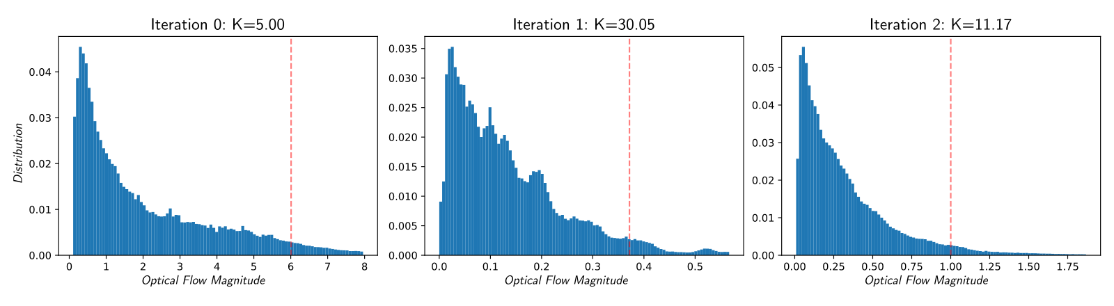
A flow-percentile heuristic chooses a rendered sampling rate, then interpolation supplies denser sensor input. Equation S8 uses approximate inverse scaling with a damped/clamped update; it is not a general convergence theorem or bound on unseen high-frequency events. The supplement describes both 200–400 fps/roughly twenty-minute and 99.8 fps/under-four-minute operating points for the example, without fully reconciling their inflection-point wording. The 60× speedup is that selected comparison. HDR images can be out of distribution for learned interpolation; reprojection/inpainting adds different artifacts.
Original mathematical definitions and modeling assumptions
In Fig. 1 (B) we rendered a test trajectory at many different frame rates and in each case interpolated the resulting data up to a common frame rate of fps. We plot the average perceptual similarity between these interpolated frames and ground truth data (lower is better), as well as the total wall time to render and interpolate these different datasets as measured using a single rendering job, on an Nvidia RTX 3080. Notice that the time it takes to interpolate the frames is dwarfed by rendering time. The overall quality of the data improves with higher frame rates and lower interpolation factors, hitting an inflection point around fps, after which there are diminishing returns as rendering time explodes. From this, we can see that for this specific scene the native frame rate is around two to four hundred frames per second, and below this rate we incur significant interpolation artifacts, as shown. It takes just under minutes to render this scene at fps and interpolate it to kHz, as compared to over four hours if we rendered every frame.
Original mathematical definitions and modeling assumptions
In practice, one would like to determine the optimal keyframe multiplier that achieves this native frame rate automatically. Prior work such as ESIM [71] addressed this by dynamically triggering a new render whenever the per-pixel optical flow exceeds a fixed threshold. While theoretically appealing, this strategy is difficult to parallelize efficiently and produces non-uniform temporal sampling that is incompatible with many video interpolation methods and sensor modalities. We instead propose a simple yet highly effective closed-form iterative approach. Under the first-order approximation that the optical flow magnitude scales as — i.e., speeding up the frame rate by reduces frame-to-frame motion proportionally — we can estimate the corrected multiplier needed to scale the flows to a target value :

Original selectable equation (S8)
Equation S8
| (S8) |
Original mathematical definitions and modeling assumptions
where is the measured -th percentile flow magnitude at multiplier , the subscript denotes clamping to the range to prevent over or under shooting, and acts as a dampening factor, with typically set to . When there is no dampening or clamping, this equation reduces to directly scaling the keyframe multiplier by the multiplicative factor, which would — if flow is perfectly inversely proportional to — result in the target flow. The added terms help with convergence when this assumption breaks down.
Original mathematical definitions and modeling assumptions
To estimate , we need to render the optical flow of the full trajectory; however, this is much cheaper than rendering the full image frames. Not only can we speed up rendering by using a very low number of samples-per-pixel and disabling auxiliary passes, but we can also render at a proportionally smaller resolution and then scale up the flow fields accordingly. In practice, this technique converges to the desired operating point in just a few iterations, making it inexpensive to execute as a pre-processing pass before any full-scale rendering begins. As an example, on the scene in Fig 1 (B), this technique finds, in just two iterations, that to achieve a -percentile flow of less than two pixels we should use a keyframe multiplier of , meaning a native frame rate of fps, perfectly matching up with the inflection point on the plot. Rendering at this frame rate and interpolating up to the target rate of fps reduces the total simulation time from 4 hours and 3 minutes to just under 4 minutes, a speedup.
Original mathematical definitions and modeling assumptions
Fig. 2 illustrates the convergence of this procedure on the classroom scene [4] with a target flow magnitude of px. Starting from an initial multiplier of , the measured 95th-percentile flow is px — well above target, indicating the frame rate is too low. Following Eq. S8, the multiplier is updated to ; however, the flow distribution shifts and concentrates near px, yielding a 95th-percentile of only px, meaning we have overshot the target. A final update produces , for which the 95th-percentile flow lands precisely at the px target.
S.3 Physically accurate sensor emulation
Conventional/high-speed/stereo models reuse camera formation; passive SPAD sampling, active photon timing, event thresholds, inertial drift, iToF taps and thermal dynamics add modality-specific stages. These are chosen forward approximations. More complex optical/electronic effects, automatic camera control and neural ISP behavior are not uniformly implemented or calibrated.
Original mathematical definitions and modeling assumptions
The brightness of a conventional CMOS camera pixel can be modeled as a function of the scene radiance over the exposure time transformed by the camera’s optical stack and response function , which encapsulates the camera response curve, tone mapping, quantization, and proprietary image signal processing [29]. Specifically, over an exposure time , a CMOS pixel will accumulate charge, and potentially saturate once it reaches its full well capacity (FWC). This process is subject to many sources of noise, including read noise and photon shot noise, which we absorb into . The intensity of the pixel can be modeled as:

Original selectable equation (S9)
Equation S9
| (S9) |
Original mathematical definitions and modeling assumptions
High-speed cameras: Usually, also based on CMOS technology, high-speed cameras can be emulated similarly to conventional cameras. However, these suffer from low signal, as the integration time is short, and readout noise that can be an order of magnitude larger than their conventional counterparts11 1 For example Scimedia’s MiCAM03-N256 has readout noise of up to . Thus, we can use the same model, and adapt and accordingly.
Original mathematical definitions and modeling assumptions
Specifically, we emulate a single-photon avalanche diode-based camera, as these are rapidly becoming mainstream thanks to their CMOS-compatible fabrication process [95]. These are binary devices that do not suffer from read noise as they are entirely shot-noise-limited. However, SPC pixels reset after a photon detection event, during which no new photons can be detected. This effectively quantized the pixel’s output, leading it to follow a Bernoulli distribution parameterized by [21], where is the scene’s radiant flux. By using the high-speed interpolated frames as a proxy for scene flux, we can emulate an SPC by sampling this distribution. Doing so accurately involves rectifying the tone-mapped frames to their linear intensities and accounting for other non-idealities such as dark count rates or low fill factors. See the supplement for more.
Original mathematical definitions and modeling assumptions
In practical single-photon LiDARs, not all photon arrivals are converted to photon detections due to sensor dead time. We explicitly model the detector’s dead time using a non-paralyzable dead time model where photons arriving within the recovery period are discarded. Our implementation can easily be extended to support paralyzable dead time. These functionalities accurately reproduce pile-up distortion, which is essential for emulating physically accurate LiDAR measurements and validating robust estimation algorithms. In addition to simulating raw photon timestamps, the simulator supports both standard Equi-width histogramming (EWH) methods and more recent Equi-depth histogramming (EDH) methods [40, 75].
S.4 Data storage and ML framework integration
A transforms.json-style metadata index records intrinsics, poses and modality asset paths. Binary photon frames are bit-packed into a memory-mapped NumPy array, giving eightfold lossless reduction relative to byte-per-binary-pixel storage, not an eightfold advantage over every possible compressed codec. Random pixel access can avoid full-frame decode. The provided loading utilities support downstream learning frameworks.
Original mathematical definitions and modeling assumptions
Both are based around maintaining a transforms.json file which encodes details about the camera’s intrinsic parameters, such as its resolution, focal length and principal point as well as a list of camera poses and asset paths for each instant of the camera trajectory. In its simplest form, these asset paths are just relative paths to the rendered image [59]. This format can be extended in a sensor-agnostic way, by allowing these asset paths to be more complex to account for other sensor modalities and ground truth annotations. For instance, events are encoded as a stream of tuples encoding the time, x/y-coordinates, and polarity of the event, which are saved in a separate file that can be linked to.
Original mathematical definitions and modeling assumptions
To overcome these issues, we store all SPC data as a single large bitpacked numpy array. In this manner, the data is losslessly compressed by and can be memory mapped which enables fast random access to the whole dataset. Since the minimum addressable unit of memory is a byte, we are forced to read in a whole byte, whether it represents eight pixels or only one. Thus this compression scheme has virtually no runtime costs, and decompression can be performed on the fly when accessing pixels. VisionSIM abstracts away the tricky bitmasking operations required to perform this compression, instead exposing a high-level API to read and write SPC data directly.
S.5 Forward models and implementation details for selected sensors
The detailed forward models specify the measurement abstractions used in emulation. All formulas and source mathematical context remain, including temporal photon rates, normalized correlation functions and the thermal detector derivation. Physical realism is limited by the correctness and calibration of those inputs/approximations.
S.5.1 Emulating single-photon cameras
Under constant exposure flux, a binary SPAD observation is Bernoulli with probability 1−exp(−phi·tau). Input intensity must be linearized and mapped to a photon-rate scale. The correction factor absorbs uncalibrated brightness, dark counts and fill effects; ordinary tone-mapped video alone does not identify all device parameters or supply absolute radiometry.
Original mathematical definitions and modeling assumptions
Assuming constant flux during the exposure time, the number of photons incident on a pixel during an exposure time follows a Poisson distribution parameterized by the total incident light during that exposure, namely , where is the scene’s radiant flux. A SPAD-based SPC does not suffer from read noise; however, its pixels reset after a photon detection event, during which no new photons can be detected. This quantizes the pixel’s output, leading it to follow a Bernoulli distribution with parameter [21].
Original mathematical definitions and modeling assumptions
Therefore, SPC can be emulated by Bernoulli sampling the interpolated intensity frames. However, the ground truth frames do not encode scene flux; they encode the scene’s intensity, often non linearly. We must first ensure the frames are in a linear colorspace, either by generating them as such or undoing any tone mapping that may have been applied. This intensity then needs to be mapped to scene flux; however, up until now, there has been no concept of scene brightness in absolute terms. While a user can set the power of every light source in Blender, this does not translate directly to physical units. Instead, we introduce a correction factor that maps a pixel’s linear intensity to a flux value, absorbing into it any non-idealities such as dark count rates or low fill factors.
S.5.2 Active single-photon camera modeling
The active model forms geometric transients, convolves source/instrument response, adds ambient photon arrivals and applies detection/readout behavior. It supports equi-width and equi-depth histograms. Stochastic arrival/detection is separate from differentiable execution modes; the paper demonstrates fitting an IRF, not differentiability of every discrete sampled event under arbitrary settings.
S.5.2.1 Forward model implementation details
Albedo/depth and field-of-view masks define the transient; source IRF and spectrally filtered ambient flux define arrival rates. Non-paralyzable recovery, timing resolution and readout compression then shape measurements. PyTorch vectorization and unit-aware configuration help implementation, while compact notation still requires a consistent rate-versus-bin-count convention. End-to-end parameter optimization is an available mode rather than a reported broad hardware-design benchmark.
Original mathematical definitions and modeling assumptions
The photon-transient is the scene response function (SRF) modeling the interaction of an ideal laser pulse with the scene. In VisionSIM we utilize ground-truth data (RGB albedo and depth maps) generated by the rendering engine. To bridge the discrete spatial domain of the renderer and the temporal domain of the SPAD, we employ a per-pixel Field-of-View (FOV) integration method. For every sensor pixel , we accumulate the weighted contribution of scene points within its projected cone. The simulator defines a weighted per-pixel FOV mask, , which encapsulates the geometric relationship between the scene and the sensor optics22 2 We explain the forward imaging model for a single pixel and drop the subscript .. For each pixel, the discrete scene response at bin index aggregates the radiometric contributions of scene points within a field-of-view mask as

Original selectable equation (S10)
Equation S10
| (S10) |
Original mathematical definitions and modeling assumptions
where is the temporal bin width, is albedo, the inverse-square falloff, the mask weight, and the quantum efficiency. This mask-based approach allows us to simulate realistic lens effects, such as vignetting and blooming, which are critical artifacts in robotic perception pipelines.
Original mathematical definitions and modeling assumptions
The raw scene transient assumes an ideal impulse illumination. To model the active source, we convolve the transient with the system’s Instrument Response Function (IRF) represented by . The simulator supports parametric pulse shapes (e.g., Gaussian, Square) or empirical IRFs derived from hardware calibration. Robotic platforms often operate in uncontrolled lighting (e.g., direct sunlight). We model ambient light not as additive noise, but as a distinct photon source. The simulator configures spectral bandpass filters, ensuring that only ambient light overlapping with the laser’s spectrum contributes to the background photon count rate, modeled as a DC offset . The resulting computation represents the expected photon arrival rate incident on the detector:

Original selectable equation (S11)
Equation S11
| (S11) |
Original mathematical definitions and modeling assumptions
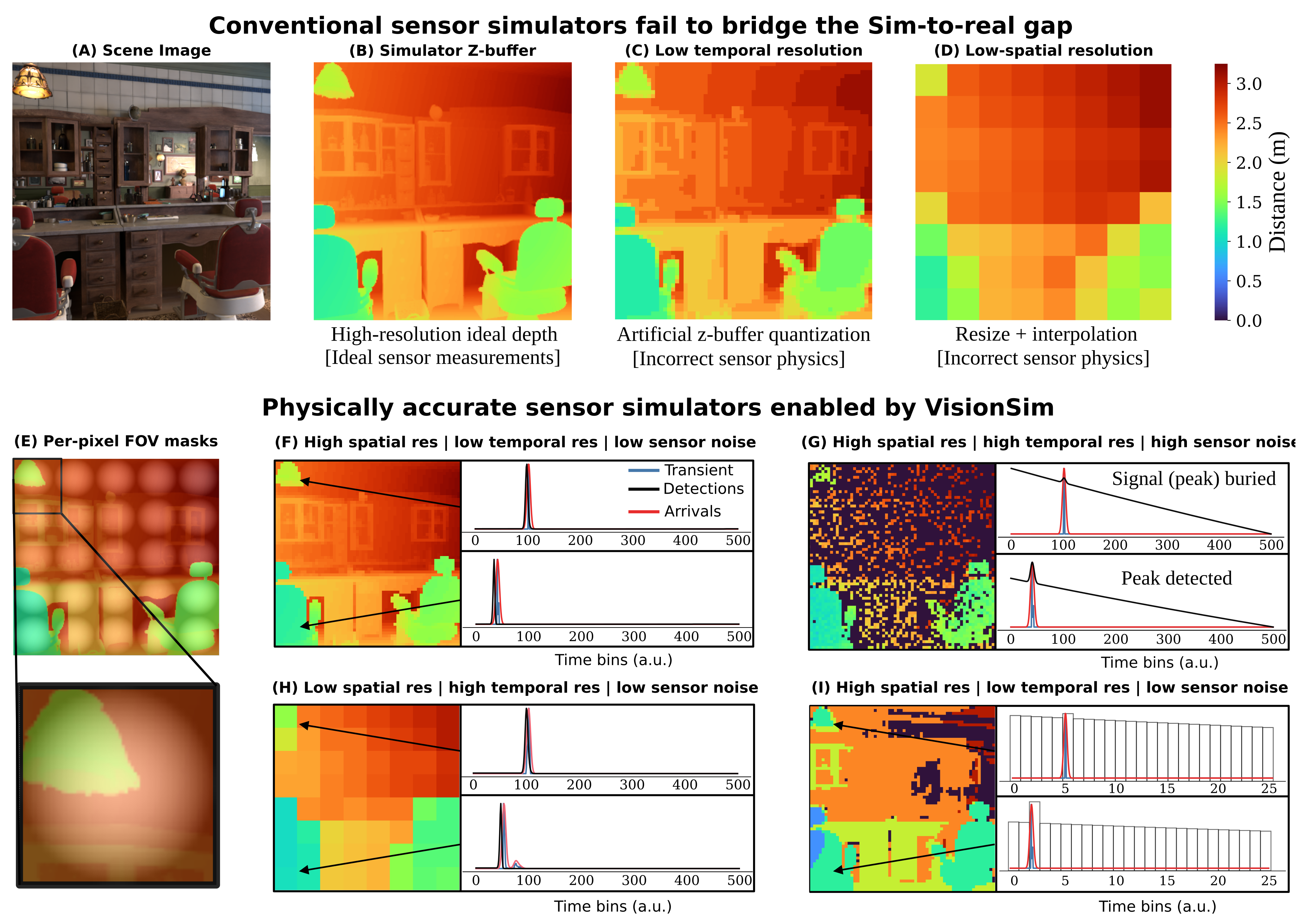
To transform continuous photon rates into discrete digital measurements, VisionSIM models the stochastic behavior of sensor electronics along with realistic hardware readout schemes. First, photon arrivals are sampled from an inhomogeneous Poisson process, where the detected count within a given time bin is distributed as to account for both active signal and ambient background flux. We explicitly incorporate a non-paralyzable dead time () model to simulate the non-linear pileup distortions typically observed when operating in high-flux scenarios. We support two different on-sensor compression methods: (i) standard equi-width histogramming (EWH), which aggregates arrivals into fixed temporal intervals, used in conventional LiDARs, and (ii) equi-depth histogramming (EDH). Designed to mitigate bandwidth constraints in high-resolution arrays, EDH utilizes adaptive quantization to dynamically vary bin widths based on local photon density, preserving high temporal resolution for sharp, peaky distributions while compressing sparse background noise. Suppl. Fig. 3 shows the effect of different readout schemes, varying FOV mask, sensor temporal resolution and sensor dead time.
S.5.2.2 Physically Constrained Single Photon LiDAR Simulations using VisionSIM
The complete multi-panel figure contrasts ideal depth, quantized/resized proxies and physically modeled field-of-view, resolution, noise and dead-time effects. Pileup can reduce counts and shift estimated range toward earlier detections. The examples demonstrate possible failure formation rather than exhaustive validation across commercial LiDAR optics and operating conditions.
S.5.3 Indirect Time-of-Flight Simulation
The full iToF derivation correlates emitted modulation and sensor demodulation with two-way travel delay. Normalization of F and the radiometric scale must be used consistently. The examples vary 35 MHz range wrapping, 50k-electron saturation, ambient light, 100 ms multi-tap motion and 10-electron read noise/12-bit quantization. These selected settings and synthetic visual results do not constitute a calibrated model for every iToF device.
Original mathematical definitions and modeling assumptions
Unlike direct time-of-flight (dToF) systems that measure the timestamps of individual photon detections, indirect time-of-flight (iToF) cameras estimate depth by emitting amplitude-modulated light and analyzing the phase shift of the reflected signal relative to the source [48]. An iToF system consists of a temporally modulated light source with radiant intensity and a sensor with a temporally modulated exposure (demodulation) function . Let be the scene depth at pixel . The radiance incident at pixel at time is given by [32]:

Original selectable equation (S12)
Equation S12
| (S12) |
Original mathematical definitions and modeling assumptions
where is the speed of light, encapsulates the scene albedo, reflectance, and inverse-square fall-off, and is the ambient light component.
Original mathematical definitions and modeling assumptions
The brightness at pixel over an integration time is the correlation between the incoming radiance and the demodulation function:

Original selectable equation (S13)
Equation S13
| (S13) |
Original mathematical definitions and modeling assumptions
where is the ambient component. is the normalized correlation function between the modulation and demodulation functions:

Original selectable equation (S14)
Equation S14
| (S14) |
Original mathematical definitions and modeling assumptions
where is the total flux emitted by the source. Finally, the measured brightness is corrupted by shot noise, quantization and other non-idealities as governed by the sensing technology.
Original mathematical definitions and modeling assumptions
By varying the modulation and demodulation functions across multiple phase offsets, the sensor captures several correlation measurements, commonly referred to as taps, to reconstruct the depth . The top row of Fig. 2 illustrates this acquisition process under ideal conditions. Here, the emulated iToF camera is using a conventional 3-tap delta-sinusoidal modulation/demodulation scheme (others such as square, ramp, Hamiltonian, and Hilbert [32] are also available within VisionSIM) with a modulation frequency of MHz, showing the ground truth RGB scene, the corresponding ground truth depth map, and the ideal correlation measurements across three phase taps.
Original mathematical definitions and modeling assumptions
Incorrect Modulation Frequency: The modulation frequency defines the unambiguous depth range of the sensor. In the figure, the incorrect modulation frequency uses MHz (yielding an unambiguous depth of only meters, which is not enough for the scene). The phase wraps around, causing severe phase wrapping ambiguities where distant objects appear deceptively close.
Original mathematical definitions and modeling assumptions
Sensor Saturation: When the exposure time is too long, or an object is highly reflective or positioned too close to the active light source, the accumulated charge can exceed the sensor’s full well capacity. This saturates the pixel and corrupts the correlation measurements. Here, clipping occurs because the full well capacity of k electrons is exceeded. This injects non-linear distortions that corrupt the reconstructed depth (notice the front row chairs and ceiling lamps).
Original mathematical definitions and modeling assumptions
Motion Blur: Because iToF systems must sequentially capture multiple frames (taps) to reconstruct a single depth map, any relative motion between the camera and the scene during the acquisition sequence leads to multi-tap motion artifacts. For this example, motion blur happens over ms. VisionSIM simulates this effect by temporally offsetting the frames used for each tap, accurately reproducing the resulting depth tearing and ghosting at object boundaries.
Original mathematical definitions and modeling assumptions
Sensor Noise and Quantization: We model physical noise sources such as shot noise and read noise, alongside the finite resolution of the analog-to-digital converters (quantization). In the figure, the noise corresponds to shot noise plus a read noise of and a -bit ADC. These factors lead to high-frequency depth noise and quantization banding in the reconstructed depth map.
S.5.4 Thermal Cameras
The thermal pipeline separates scene temperature, in-band radiance and detector response. Common cameras/geometry align visible and thermal outputs within the simulated scene, while emissivity, reflection and detector lag determine their very different appearance.
Original mathematical definitions and modeling assumptions
Long-wave infrared (LWIR, –) thermal cameras occupy a fundamentally different place in the imaging stack than the other modalities in VisionSIM: rather than measuring light scattered off the scene within the last microseconds, they measure the long-wave radiation a surface emits as a consequence of its temperature. The world simulation layer supplies that temperature field through the integrated heat-transport solver (Sec. S.2.5.2); here we describe how the sensor emulation layer turns it into a measurement in two stages: rendering the temperature field into in-band thermal radiance with a graybody shader (Sec. S.5.4.1), and applying the microbolometer image-formation model whose thermal inertia gives real LWIR video its characteristic lag and smear (Sec. S.5.4.2).
S.5.4.1 Rendering the Temperature Field into Thermal Radiance
A material override renders the same scene in the thermal band, disabling visible-only lights and using the solved temperature attribute. This preserves geometric registration. The shader still requires an emissivity/reflectance model and an appropriate in-band blackbody response.
Graybody emission shader.
Outgoing graybody radiance combines emissivity-weighted emission with complementary reflected incident LWIR radiance. The source adopts Lambertian reflection and scalar emissivity rather than measured directional/spectral reflectance. A low-emissivity metal can reflect cool surroundings, so apparent thermal brightness is not simply its physical temperature.
Original mathematical definitions and modeling assumptions
At LWIR wavelengths each surface radiates as an opaque graybody, contributing both its own thermal emission within the camera’s sensitivity band and a reflection of the long-wave radiation arriving from the rest of the scene. We model the outgoing in-band radiance at as

Original selectable equation (S15)
Equation S15
| (S15) |
Original mathematical definitions and modeling assumptions
where is the surface temperature from the heat solver, is the LWIR emissivity, is the incident long-wave radiance gathered from the rest of the scene [62], and is the camera response to a blackbody at temperature , obtained by integrating Planck’s law against the camera’s spectral response and generally well-approximated by the Sakuma–Hattori model [76, 62]. The first term is the graybody emission within the LWIR specturm, scaled by emissivity through Kirchhoff’s law; the second is its conjugate reflection, weighted by , which is exactly the reflectivity an opaque graybody assigns by energy conservation. Although the angular reflectance of real materials in the – band is not as well characterized as in the visible, we adopt a Lambertian BRDF for the reflected term: it is the canonical choice for a graybody, keeps the model fully determined by the single per-surface parameter , and is straightforwardly replaceable by a measured wavelength-specific BRDF as the literature matures. The two terms together capture the qualitative behavior of real LWIR imagery without any material-specific special cases: a polished low- metal “looks cold” because its mix weights the reflection of its cooler surroundings, while a high- matte surface reads its own emitted light almost directly.
S.5.4.2 Microbolometer Thermal Inertia
A microbolometer membrane is a first-order thermal system whose finite time constant creates lag and smear. An affine readout maps membrane response to counts; under that calibration, rendered radiance can be temporally filtered. This models inertia, not the full thermal camera noise and calibration chain.

Original selectable equation (S16)
Equation S16
| (S16) |
Original mathematical definitions and modeling assumptions
where is the membrane-to-substrate temperature difference, is the membrane heat capacity (), is the thermal conductance of its supports (), is the membrane’s in-band absorptivity, and is the instantaneous incident in-band radiative power (). The ratio has units of time and is the membrane’s thermal time constant, the natural timescale on which it equilibrates to a change in incident radiation; for commercial uncooled LWIR detectors, typically lies in the – range. Defining the hypothetical instantaneous steady state —the temperature the membrane would reach if it equilibrated infinitely fast to the radiation present at time —Eq. S16 takes the canonical first-order form

Original selectable equation (S17)
Equation S17
| (S17) |
Original mathematical definitions and modeling assumptions
The interpretation is direct: the membrane temperature chases its instantaneous target at a rate set by . The readout integrated circuit then reports a digital count that is affine in , so up to a one-time factory calibration the reported video is a temporally low-pass-filtered version of the scene radiance. Crucially, is exactly the idealized infinite-bandwidth measurement that a perfect (zero-) camera would produce—which is precisely the in-band radiance that our graybody renderer writes into each frame (Eq. S15). We can therefore synthesize a realistic microbolometer response by filtering the rendered radiance sequence through Eq. S17.
Closed-form solution and discretization.
The exponential convolution becomes an exact single-pole update for piecewise-constant frame input, with a=exp(−delta_t/tau). Exact integration of that assumed input does not recover unresolved motion between renders. At 60 fps and tau=10 ms, a≈0.189: a step reaches about 81% after one sample and 96% after two, so the text’s approximate three-frame/90% description is coarse. Interpolated substeps change the assumed input, while the complete derivation and limits remain.

Original selectable equation (S18)
Equation S18
| (S18) |
Original mathematical definitions and modeling assumptions
Equation S18 says that the current membrane temperature is a weighted average of all past radiance, with weights given by a decaying exponential of timescale : recent radiance contributes strongly, while radiance from many ago has been “forgotten.” This is the precise sense in which the bolometer acts as a temporal low-pass filter on the scene.
Original mathematical definitions and modeling assumptions
To apply this to rendered video, we discretize Eq. S18 at the frame rate. Let with , let denote the rendered input at frame , and let denote the filtered output we want to compute. Splitting the convolution integral at the previous frame time and factoring the exponential kernel as gives

Original selectable equation (S19)
Equation S19
| (S19) |
Original mathematical definitions and modeling assumptions
where the first term is exactly what the convolution from to contributes, attenuated by one frame’s worth of exponential decay. The renderer samples the scene once per frame with no within-frame motion blur, so we model the input as piecewise-constant across each interval (a zero-order hold), for . Pulling out of the integral and evaluating collapses Eq. S19 to a single-pole infinite impulse response low-pass filter,

Original selectable equation (S20)
Equation S20
| (S20) |
Original mathematical definitions and modeling assumptions
For piecewise-constant input this is the exact integrator of Eq. S17, not a finite-difference approximation, and the only free parameter is the single dimensionless ratio that determines . The limits are sanity-checking: (instant camera) gives and , so the output equals the input with no lag; (infinitely sluggish camera) gives and , so the output is frozen. In the regime of interest, at and , and a hot pixel reaches of its steady response in about three frames; larger stretches the lag proportionally. When (a fast detector under a slow render) the zero-order hold becomes inaccurate, and we instead linearly interpolate the input between rendered frames and run substeps per frame with , recovering Eq. S20 at .
Scope of the thermal sensor model.
Current thermal sensing models scalar graybody/Lambertian response and temporal inertia. NETD-related temporal noise, fixed-pattern/column structure, focal-plane drift, flat-field correction effects, vignetting and self-emission are left for future work. The selected cup fidelity result should be read within this scope.
Original mathematical definitions and modeling assumptions
Our graybody shader (Eq. S15) assumes a Lambertian BRDF and a single scalar emissivity, whereas real materials exhibit angularly and spectrally varying reflectance in the – band that is far less characterized than in the visible. On the detector side, our current model captures only the microbolometer’s thermal inertia, the first-order temporal low-pass that produces motion smear, and not the temporal noise families that define the NETD [64], the spatial fixed-pattern and column-stripe structure, the focal-plane-array drift between flat-field corrections, vignetting, or narcissus-like self-emission; some of these could be layered onto the rendered radiance as a post-process following the standard sensor signal chain, which we leave to future work.
S.6 Building Digital Twin of Commercial dToF LiDAR
A single ADAPS ADS6311 scene tests a physically parameterized twin. IRF fitting and independently measured optical glare improve agreement, but scene reconstruction and material overrides are also calibrated choices. The study does not establish out-of-device or broad out-of-scene transfer.
S.6.1 Capture Setup
The device has 256×192 output with 3×3 SPAD binning, approximately 11 ns dead time and 754 ps temporal resolution. A retroreflective stop sign exercises strong-return pileup and optical glare. Detector recovery and internal optical scattering are distinct causes of the observed artifacts.
Original mathematical definitions and modeling assumptions
For this evaluation we captured the real scene using an off-the-shelf, commercial, single photon LiDAR developed by ADAPs Photonics [1] (the ADS6311) used because it gives access to raw unprocessed histograms. The ADS6311 is a 1D scanning LiDAR with a resolution of with spatial binning to improve SNR (i.e. there are SPAD elements). This device has a dead-time of ns and a temporal resolution of ps. The transmitter uses VCSEL laser diodes to scan a 6-row-wide band in the vertical direction.
S.6.2 Blender Simulated Scene
A Blender approximation matches geometry and camera placement, with an approximate lens model and manually increased sign albedo because true retroreflection is not directly supported. Background/tarp mismatch remains. The result is a calibrated scene/device example, not a fully general retroreflective material implementation.
S.6.3 Learning the Impulse Response Function
The IRF is fitted for 1000 epochs using a 20×20 patch from one background-tarp scene, with cross-correlation and a stated smoothness term. The exact printed loss remains; its normalization/TV convention is not fully specified. This demonstrates response fitting under the selected scene/calibration assumptions, not joint identification of every optical and electronic parameter.

Original selectable equation (S21)
Equation S21
| (S21) |
Original mathematical definitions and modeling assumptions
where is the pixel-wise cross-correlation between the predicted (simulated) histogram and measured histogram across a patch, and the total variation term is a smoothness penalty between adjacent bins to avoid sharp spikes in the IRF. The comparison given in Figure 4 shows the measured histogram as compared to a simulated histogram using our learned IRF for a point on the stop sign and a point in the region containing glare artifacts.
S.6.4 Comparison to Real Capture Details
Glare uses 49 measured PSFs and distance-weighted spatial interpolation; it is measured rather than learned by the IRF optimizer. Supplementary error maps show RMSE 0.87→0.77→0.74→0.54 as effects are added. Their tighter region of interest deliberately reduces challenging background mismatch, so that 0.33 m change differs from the main text’s roughly 1.53 m improvement. Neither crop should be silently substituted for the other.
S.7 Dataset generation interface
The curated scenes are rigged/physics-baked; the pipeline records explicit configurations, dispatches parallel Blender jobs and post-processes sensor outputs. The exact eight-line command remains copyable, with both complete API examples retained in Figure S1. Reproduction depends on the pinned Blender/library/container release and available assets/configurations. Permissive scene-asset licenses and the primary software repository’s GPL license are distinct releases.
Original mathematical definitions and modeling assumptions
Asset curation. To help accelerate research, we release all D assets and scripts used to create sensor-realistic datasets, lowering the need for manual asset curation, which can be a significant hurdle. Specifically, we release the high-quality rigged scenes, some of which are shown in Fig. 5, which have been used to create the VisionSIM dataset. These scenes have mostly been crowdsourced from sites such as BlendSwap [60] or Blender’s example scenes [4], although some have been made or heavily modified specifically for this use case. All scenes are fully rigged, physics-baked, and validated to render without modification using the Blender version pinned to the corresponding VisionSIM release. These assets are released under the Creative Commons license (CC BY 4.0) or similar permissive licenses.
Original mathematical definitions and modeling assumptions
Generation pipeline. Dataset generation is driven by a single script, scripts/mkdataset.py, that wraps the same RenderConfig dataclass and render_animation backend used throughout VisionSIM’s CLI. A user specifies a directory of blend-files and an output directory; the script then (i) uniformly samples non-overlapping sub-trajectories from the animation range of each scene, or renders the whole trajectory if desired, (ii) dispatches each (scene, trajectory) pair as an asynchronous render job via BlenderClients.pool, and (iii) saves every sequence under a deterministic path which also contains the explicit configuration used to produce the sequence. All relevant metadata are stored in per-modality SQLite databases alongside the raw data. The RenderConfig dataclass exposes every relevant parameter — resolution, render device, keyframe multiplier, types of ground truth, noise threshold, and per-modality flags — entirely through the CLI, so a full reconfiguration of the dataset requires no code changes. For example, to render a dataset at fps with depth, normals, optical flow, and segmentation using five parallel jobs:
python scripts/mkdataset.py create-datasets \
  --scenes-dir=scenes/ --datasets-dir=datasets/ \
  --sequences-per-scene=1 \
  --render-config.width=800 --render-config.height=800 \
  --render-config.depths --render-config.normals \
  --render-config.flows --render-config.segmentations \
  --render-config.keyframe-multiplier=4.0 \
  --render-config.jobs=5