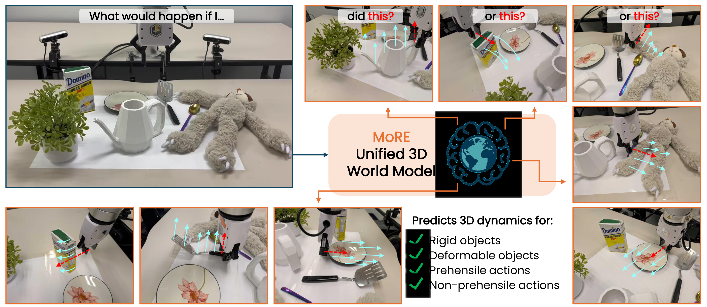
At a glance
MoRE predicts manipulated-object motion from histories of object and tool point clouds. A shared representation feeds three motion experts: rigid non-prehensile, deformable non-prehensile, and deformable prehensile. A supervised router chooses an expert from observed interaction history, combining a rigid transformation constraint with free-form deformation models.
Training mixes simulated and real interactions. The model improves reported geometric prediction metrics and supports model predictive control (MPC) for box pushing and toy manipulation. The reported 20 frames per second refers to model inference, not a demonstrated 20 Hz perception-and-planning control loop.
1. Introduction
Manipulation prediction must accommodate both material behavior and contact type. A single unconstrained predictor can distort rigid objects, while a rigid model cannot represent squeezing or stretching. MoRE addresses this conflict by sharing scene and motion features while separating output rules according to physical regime.
The contribution is a unified predictor over three selected regimes and multiple tools, with learned routing at inference. It does not cover every material or manipulation category: rigid grasping and simultaneous interactions among multiple manipulated objects are outside the modeled scope.
2. Related work
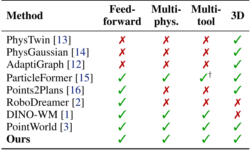
Table 1 preserves the authors’ comparison of feed-forward prediction, material diversity, tool diversity, and 3D representation. These capability labels summarize heterogeneous systems and are not themselves a controlled quantitative benchmark.
3.1. Problem formulation
Equation 1 defines future object point clouds from current state, current tool geometry, and a finite state/action history. Actions are represented by the tool’s full point cloud, obtained from robot commands through forward kinematics. This abstracts away particular joint coordinates while still requiring the tool geometry and kinematic mapping.
The implementation uses eight history steps, a three-step prediction horizon during training, 150–512 object points according to object size, and 100 end-effector points. Longer predictions feed generated states back into the history buffer.
Equation

3.2. Mixture of motion experts
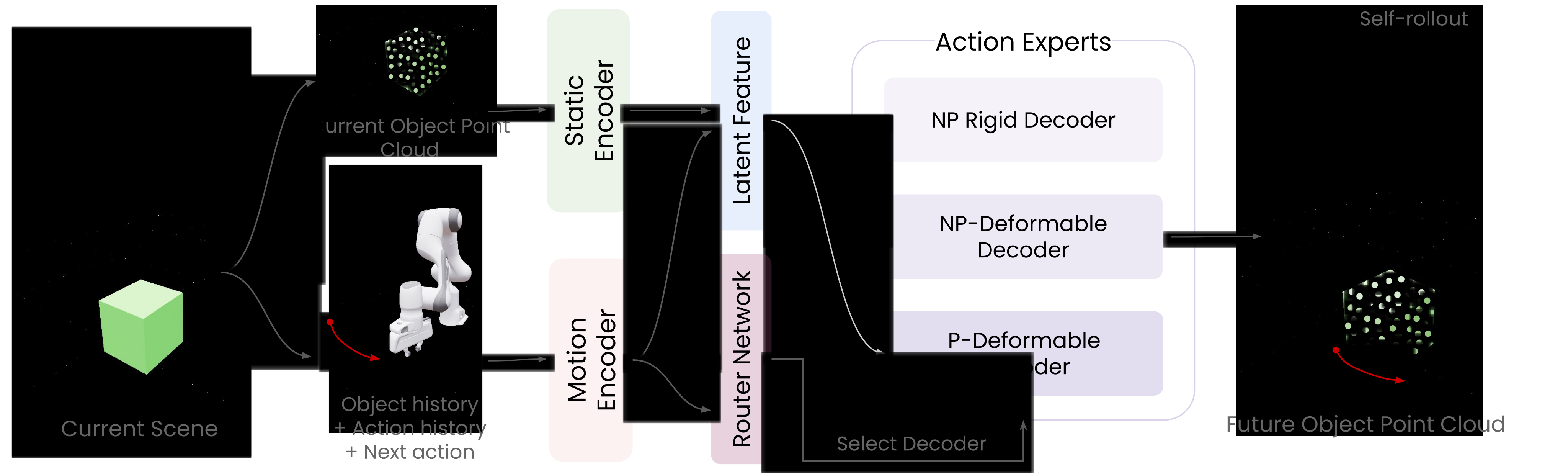
Static geometry and motion features are fused into a shared representation. A gating network predicts a one-hot selection over three experts; Equation 2 retains the selection constraint. The main method re-evaluates this router at each rollout step, allowing the selected regime to change.
Hard routing selects one expert’s prediction rather than averaging incompatible rigid and deformable outputs. Expert labels supervise routing during training; test-time selection uses observed motion history rather than a supplied interaction label.
Equation

3.3. Physics-aware experts
The experts cover rigid pushing or pulling, deformable pushing or pulling, and deformable grasping. Rigid prehensile interactions are omitted under the authors’ assumption that negligible-slip rigid grasping has relatively little motion uncertainty. This assumption limits the scope of the three-expert decomposition.
Rigid expert
The rigid head predicts a global rotation and translation, using a continuous six-dimensional rotation representation. Applying the same rigid transform to every object point preserves internal distances and prevents arbitrary geometric distortion. Zero rigidity error is therefore partly built into the output representation, rather than independent evidence that all contact dynamics are correct.
Deformable experts
Two separate heads predict pointwise 3D displacements with the same architecture but different parameters. One specializes in sustained grasping interactions; the other models deformation under pushing or sliding. They can represent local shape change but do not impose a complete constitutive material law.
3.4. Training
Self-rollout training uses predicted states as subsequent inputs, with gradients detached through those rolled-in predictions [63]. Equation 3 combines point reconstruction error across the rollout with supervised expert-selection cross-entropy. Experts and the router are warmed up separately, then jointly fine-tuned on mixed data.
The main text describes simulation pretraining for each expert, while the appendix’s simulation generation describes non-prehensile interactions. It does not fully explain the corresponding prehensile simulation data or give a complete optimizer, training schedule, and split specification.
Equation

Autoregressive inference
Starting from an observed object state and history, each prediction is appended to a rolling buffer and becomes the next input. The process repeats to the chosen horizon. This avoids test-time dynamics fitting, but predictions can still accumulate error when rolled out beyond observed states.
3.5. Planning
MPC samples candidate tool trajectories, predicts their object trajectories, and selects the plan with the lowest goal cost. The robot executes an initial action, observes the outcome, and replans. Chamfer distance to the target object point cloud measures task progress; an additional obstacle cost may be used.
The appendix adds a necessary initialization step: random probing interactions generate motion history for routing. Thus a static image or point cloud alone is insufficient for the reported system’s initial regime identification.
4.1. Implementation
Training uses about 20,000 simulation episodes and 7,000 real episodes, sampled with a fixed 1:1 simulation/real mixture. The main text cites DROID and AdaptiGraph for real data, while Appendix A identifies DROID and the Particle-Grid Neural Dynamics (PGND) dataset. The edition retains this source discrepancy rather than treating the provenance descriptions as identical.
Simulation covers roughly 300 rigid objects, 300 deformable objects, and 30 tools. Physical properties and action noise are randomized. The static geometry encoder is frozen; motion encoding, fusion, routing, and output heads learn the dynamics.
4.2. Tasks and metrics
Evaluation covers the three expert regimes. Geometric metrics compare predicted and reference point clouds; the tables label the correspondence metric as root mean squared error (RMSE), although parts of the prose and captions call it mean squared error (MSE). Chamfer distance (CD) evaluates unordered geometric agreement.
Rigid error is residual alignment error after fitting a rigid transform. Deformable evaluation uses a Laplacian error. These are geometric or structural proxies, not direct measurements of force accuracy or physical safety.
4.3. Dynamics results
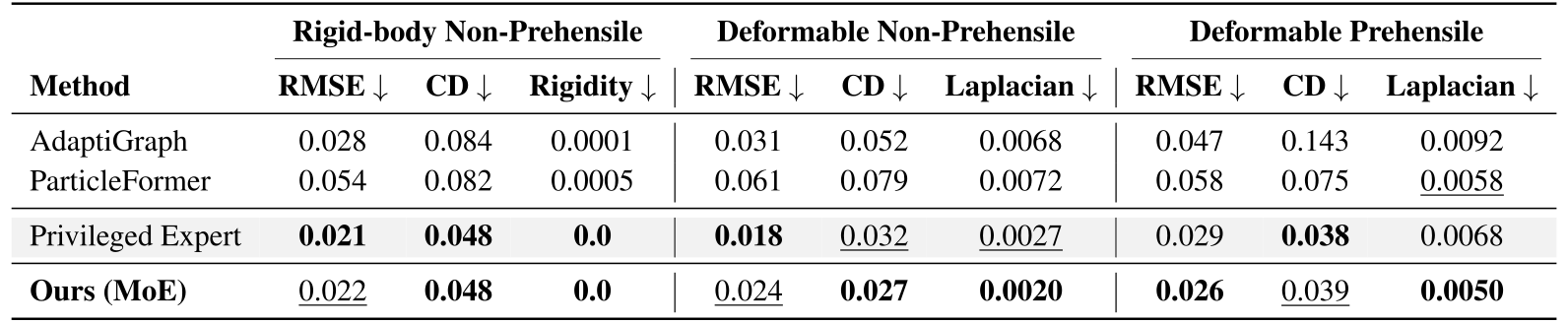
Table 2 shows better geometric and structural metrics than AdaptiGraph and ParticleFormer across the listed regimes. Relative to privileged domain-specific experts, results are mixed: deformable non-prehensile RMSE is 0.024 versus 0.018, while CD improves from 0.032 to 0.027. Learned routing approaches specialized performance without winning every metric.
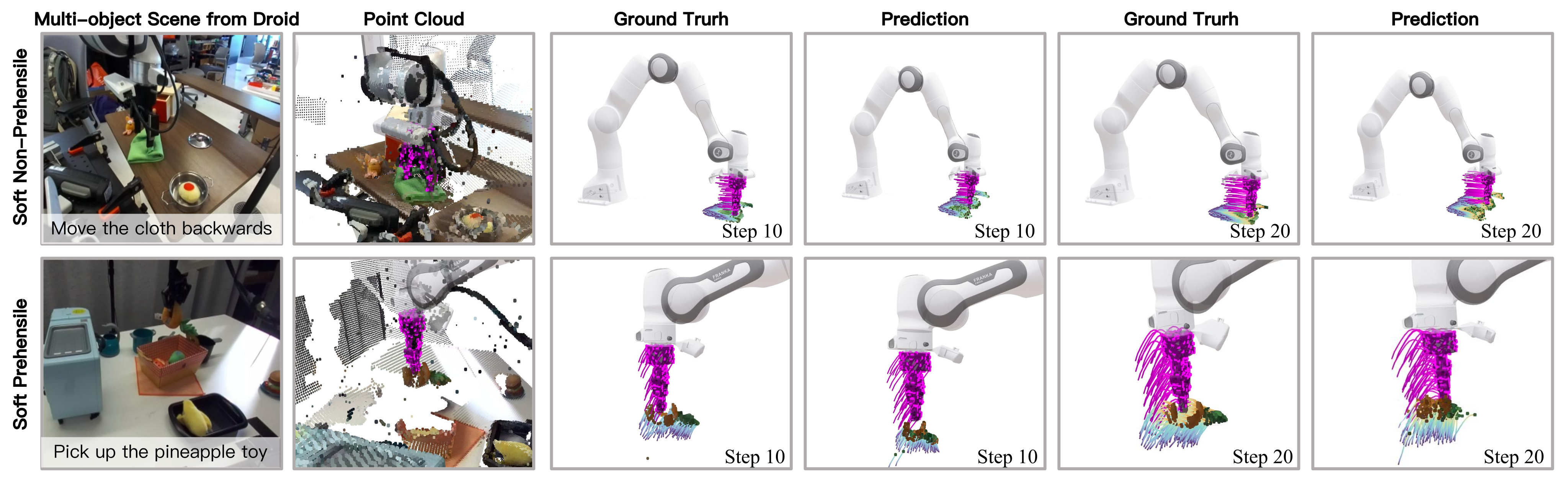
On DROID, Table 4 compares only moving target-object points, not whole-scene flow. MoRE’s RMSE is 0.023/0.014/0.021 across the three regimes, versus PointWorld’s 0.031/0.028/0.029. It also improves the listed CD and structural errors. Figure 3 preserves the cluttered-scene examples, including small and partially observed target objects.

4.4. Expert and routing ablations
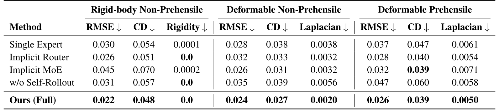
Capacity-matched ablations compare a single expert, soft implicit routing, an implicit mixture inside the Transformer, and training without self-rollout. The complete model has the best or tied-best values in Table 3.
Removing self-rollout increases deformable prehensile RMSE from 0.026 to 0.047. The comparisons support explicit regime-specific heads, supervised hard routing, and training on predicted states as useful components of this implementation. They do not establish that all soft mixtures or shared models must fail.
4.5. Real-world control
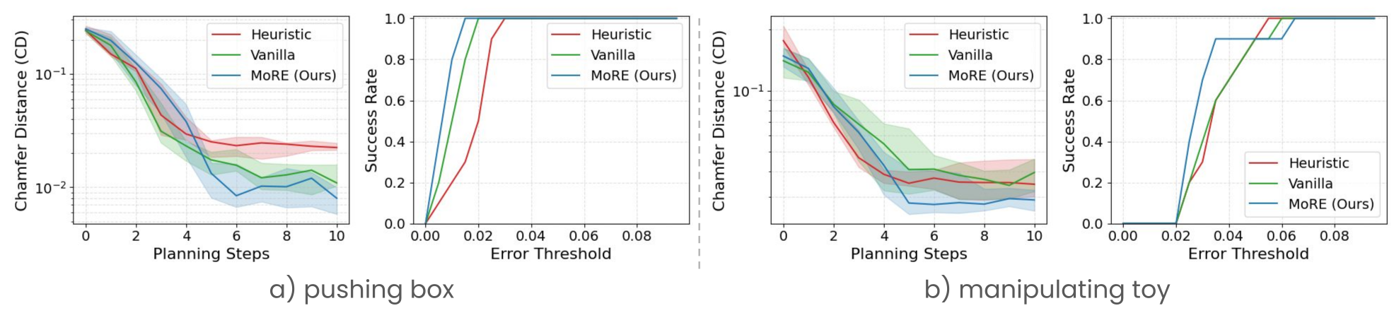
Real-robot experiments use rigid box pushing and deformable toy-sloth pose matching, with goal point clouds and CD-based success thresholds. Baselines are a translation heuristic and a single Transformer without motion experts or routing.
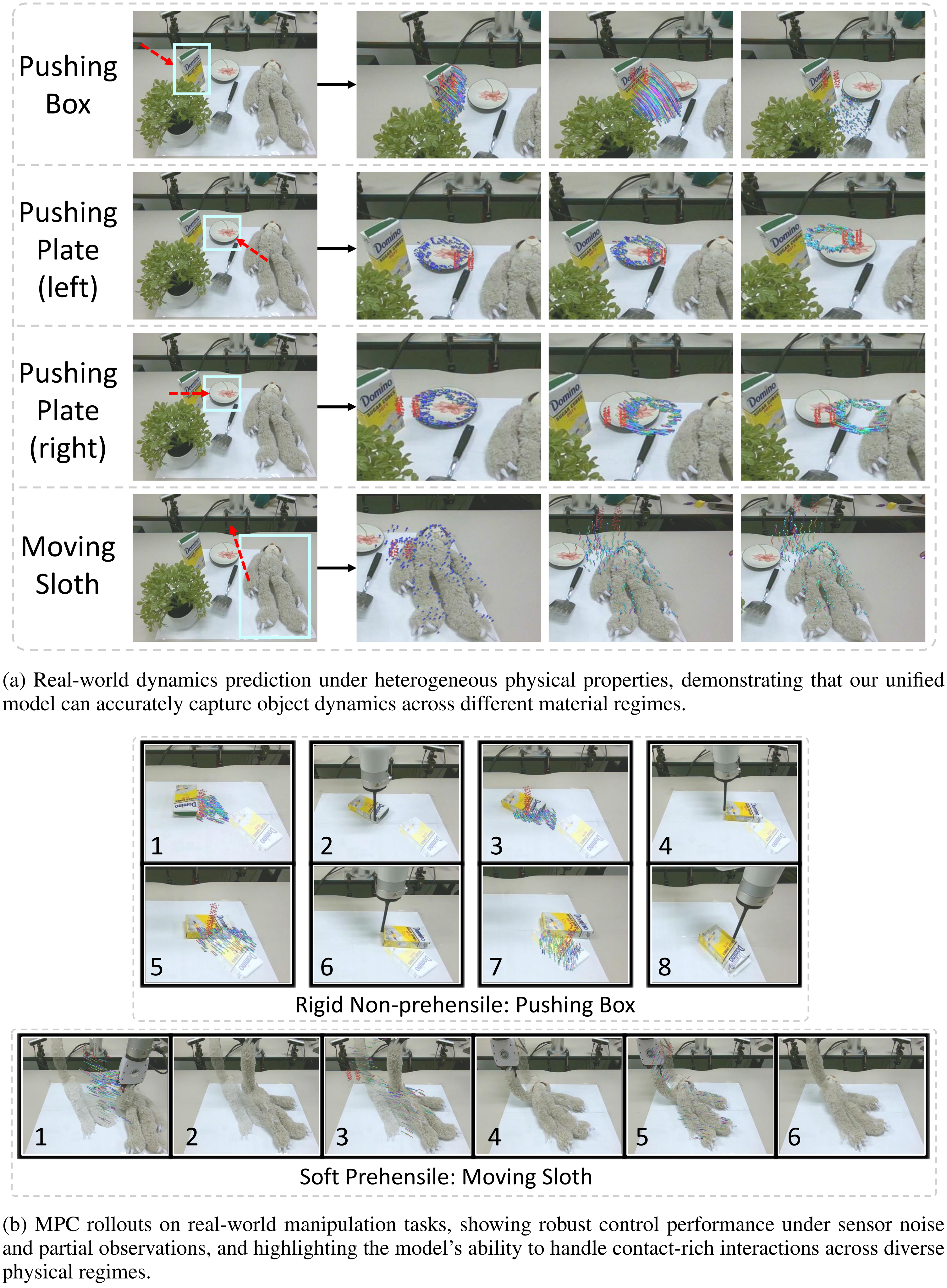
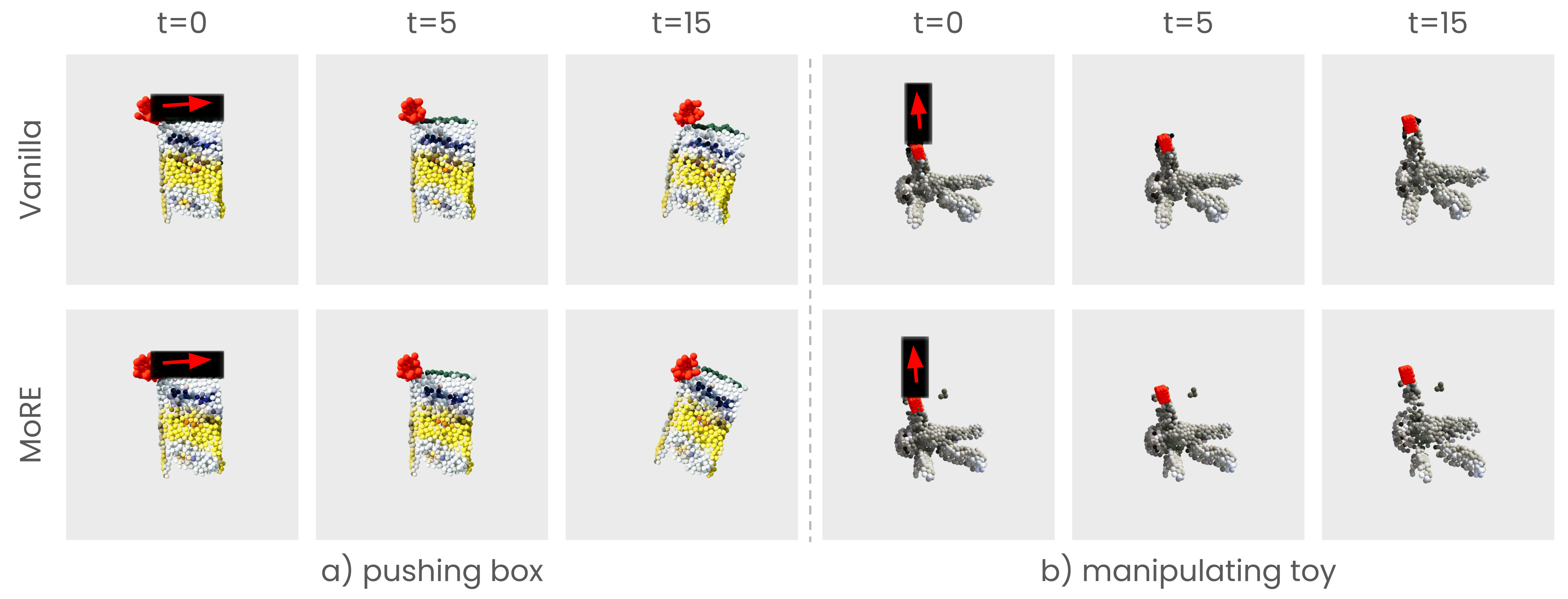
Figure 4 retains the complete error curves and success-versus-threshold plots; Figure 5 retains the prediction sequences. MoRE generally lowers goal error, especially for the rigid box. On the toy task, the success curves cross at some thresholds, so the plot does not show strict superiority at every threshold. The paper does not report repeated-seed confidence intervals or a full control-loop timing breakdown.
5. Discussion
MoRE combines a common geometric representation with specialized motion outputs. The main evidence is improved prediction on the three tested regimes and useful downstream control on two real-world task families. Its rigidity constraint and motion-history routing are central to that behavior.
Limitations
The model predicts one manipulated object at a time and does not model simultaneous multi-object dynamics. Mass, friction, elasticity, and hidden internal state are not explicitly represented; visually similar objects such as empty and filled bottles may therefore behave differently without being distinguishable from the available history.
The reported experiments leave uncertainty about broader material coverage, held-out object/tool splits, and full-system runtime. Generalization claims should be read within the described datasets and examples.
Acknowledgments
The paper acknowledges six National Science Foundation awards, computing resources from the National Center for Supercomputing Applications through Delta and Delta AI, and NVIDIA’s academic grant program.
Appendix
The full appendix’s dataset, architecture, planning, routing, and qualitative material is retained below. The project page is more-robo.github.io.
A.1. Dataset curation
Simulation and real trajectories share a point-cloud representation and are sampled equally during training. This balances controlled simulated variation with real sensing noise and contact behavior.
A.1.1. Simulation data
Isaac Lab generates interactions with approximately 300 rigid assets across 130 categories, 300 deformable assets across 100 categories, and 30 tools. Contact points and normals determine pushing and pulling directions.
Full mesh states provide temporally corresponding surface samples, reduced with farthest point sampling. Object point counts range from 150 to 512. Randomized mass, friction, deformable stiffness, and per-step Gaussian action noise diversify the training trajectories.
A.1.2. Real-world data
PGND supplies reconstructed object-motion sequences. DROID is processed through PointWorld’s scene-flow pipeline, then converted to object-centric flow: Qwen3 identifies the end-effector, manipulated object, and interaction type; SAM2 segments that object. If several masks remain, the nearest to the end-effector is selected.
This curation supplies target-object tracks and interaction labels automatically. Errors in recognition, segmentation, flow, or mask selection can propagate into the learned model.
A.2. Model architecture
Frozen Uni3D features and learned Transformer motion features each have 1,024 dimensions. Cross-attention combines the current object geometry with temporal object/tool tokens. A two-layer multilayer perceptron (MLP) produces routing logits.
The selected MLP head predicts either a global rigid transform or point displacements. This design separates geometric feature sharing from the final motion constraints.
A.3. MPC pipeline
After random interaction probes initialize history, non-prehensile planning samples 48 pushes from 16 contact points and three directions. For prehensile control, grasping is established first, then bounded tool displacements are sampled. Start/end waypoints are interpolated into dense candidate action sequences.
The planner evaluates both candidate trajectory and stopping time, allowing early termination when a predicted intermediate state better matches the goal. Real-world perception fuses four RealSense D455 cameras, applies SAM3 text-prompt masks, removes outliers with Open3D, recenters coordinates, and samples points as in training. These perception and probing steps are part of deployment even though dynamics inference needs no online optimization.
A.4. Gating evaluation
Across 50 random interactions per category, Table 5 reports selection accuracies of 95.4% for pushing, 94.9% for toy manipulation, and 99.8% for soft grasping, with 96.7% overall. The text does not fully specify how frame-level or trial-level decisions are aggregated into these percentages.

B.1. Benchmark visualization
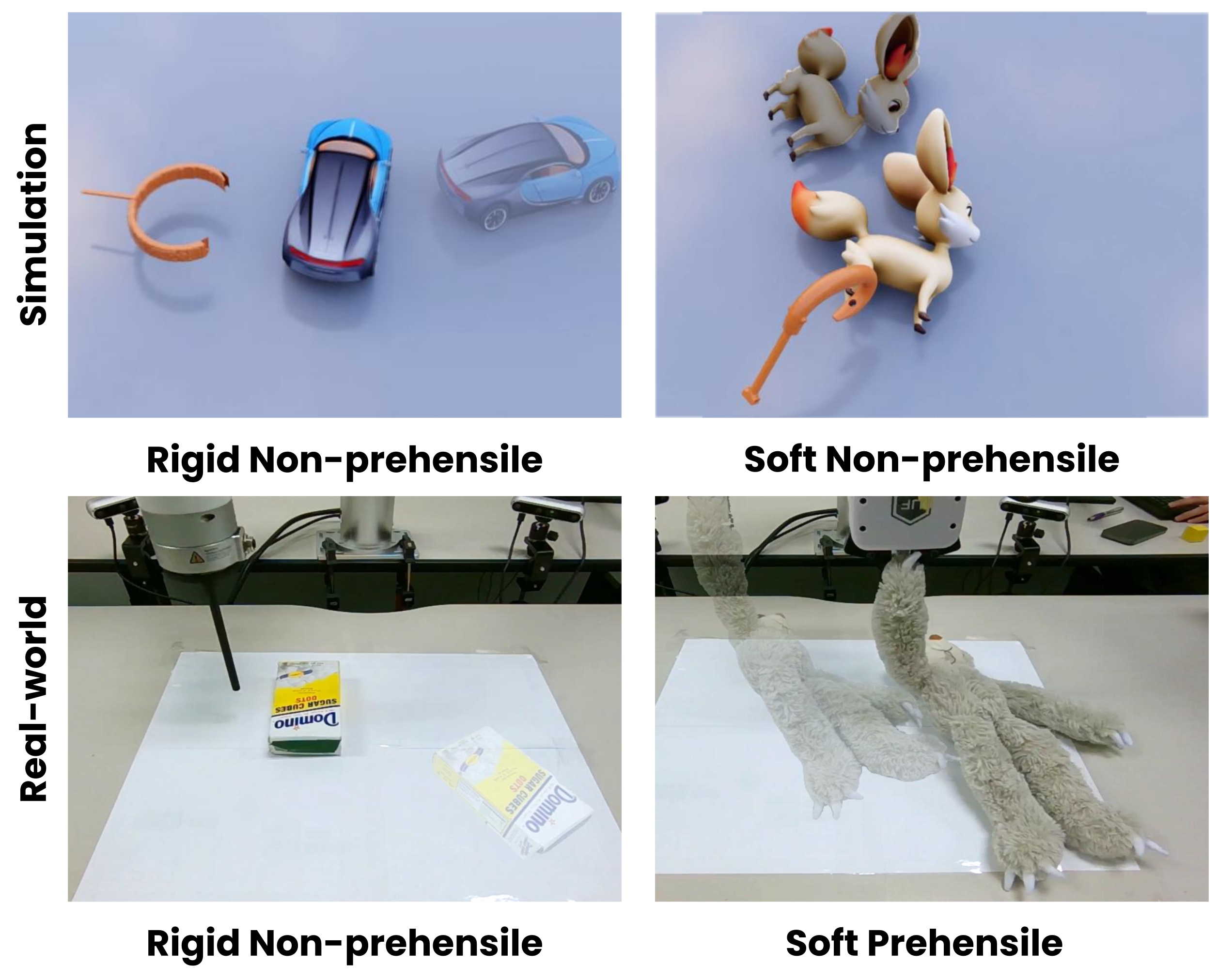
Figure 6 preserves representative simulation and real-world setups for rigid and soft objects. These examples illustrate the tested regimes and tools.
B.2. Simulation visualization
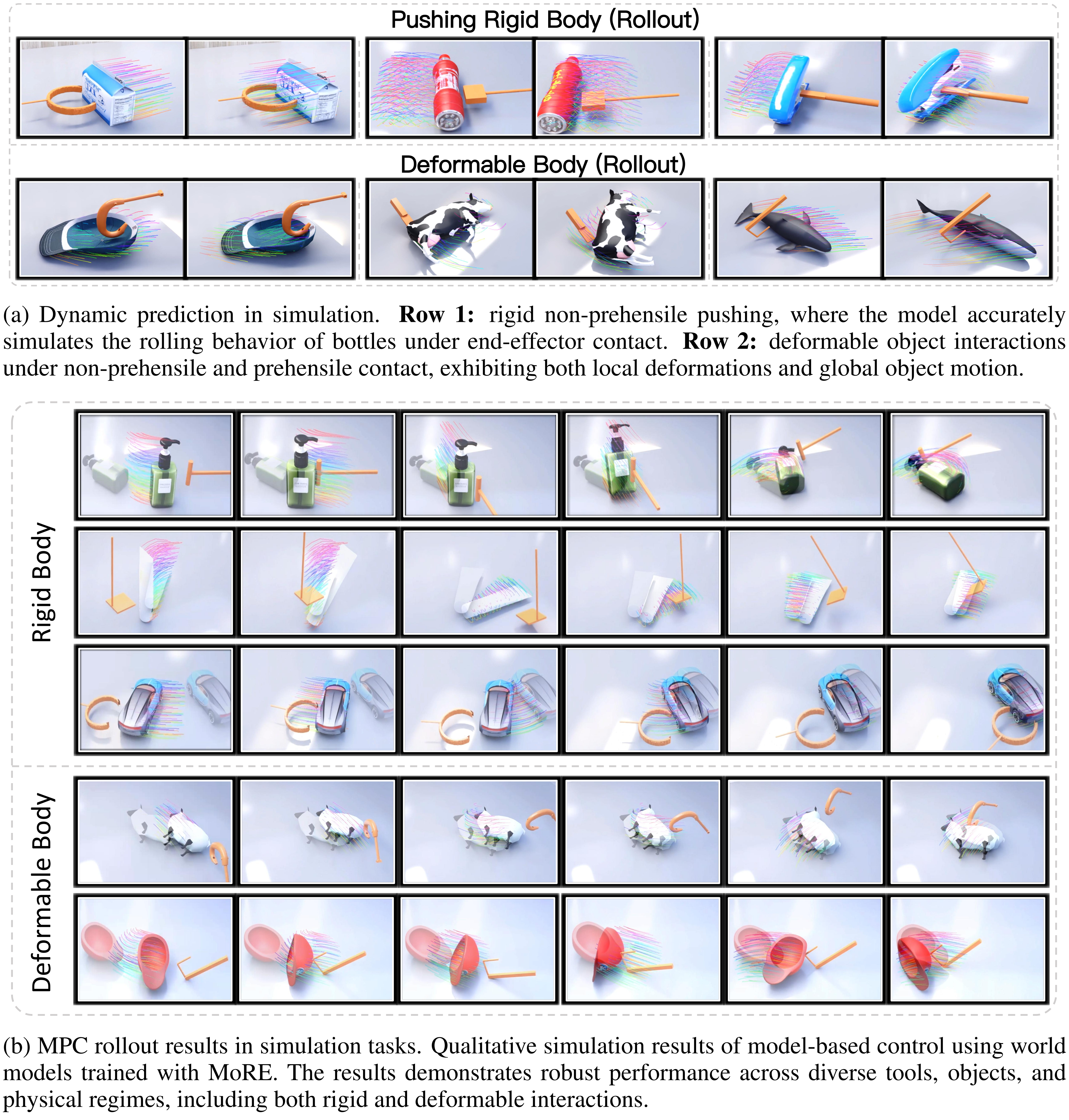
Figure 7 retains both complete panels: dynamic prediction sequences and MPC rollouts across rigid and deformable simulation tasks, including all original subcaptions.
B.3. Real-world visualization
Figure 8 retains the full real-world prediction and control sequences, including box pushing, both plate-pushing directions, and sloth movement. These are qualitative examples rather than additional independent success-rate measurements.