Literature
Display
← All papers

Machine Super Intelligence

Shane Legg

Dissertation dated · University of Lugano (doctoral dissertation) ↗

Contents

Preface and scope

Legg studies ideal agents that learn in unknown computable environments, how their performance might define intelligence, and what is lost when the agents must be computable. The dissertation combines theoretical definitions and proofs with a separate empirical study of temporal-difference learning. AIXI and the universal intelligence score are mathematical ideals; they are not directly executable algorithms or practical intelligence tests.

1. Nature and Measurement of Intelligence

What should be measured? The survey compares theories and definitions of human, animal, and machine intelligence. Legg extracts a shared emphasis on achieving goals across varied environments, while recognizing that any test depends on its interface, motivation, task distribution, and intended subject.

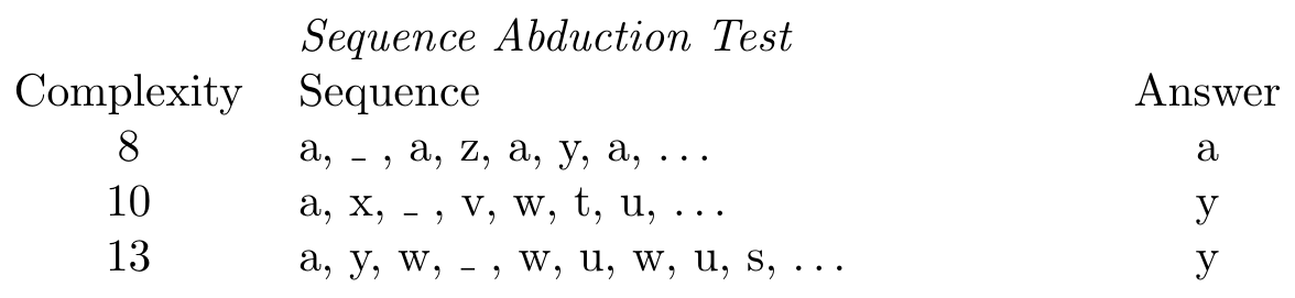
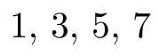
Human psychometric tests, the Turing test, task competitions, and complexity-based sequence tests each capture something narrower than unrestricted adaptive performance. A machine can be specialized to a test without exhibiting broad competence. The sequence-test examples are retained; the chapter motivates a general formal measure rather than establishing a universally accepted definition. [102, 103, 104, 172]
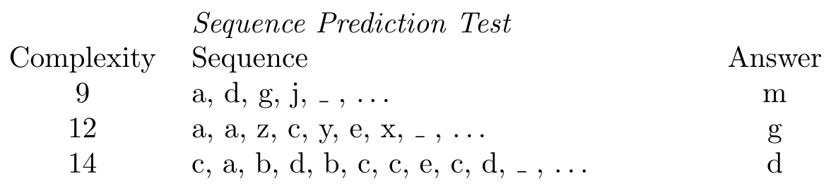
Sequence prediction test: append the next symbol; original examples, complexities and answers from Section 1.7.
Sequence abduction test: fill the missing symbol; original examples, complexities and answers from Section 1.7.

2. Universal Artificial Intelligence

From prediction to action. Bayesian inference updates hypotheses after observations. Solomonoff induction mixes computable explanations with a preference for short programs; its ideal predictor has strong convergence guarantees under a computable data-generating distribution, but evaluating the universal prior is incomputable.

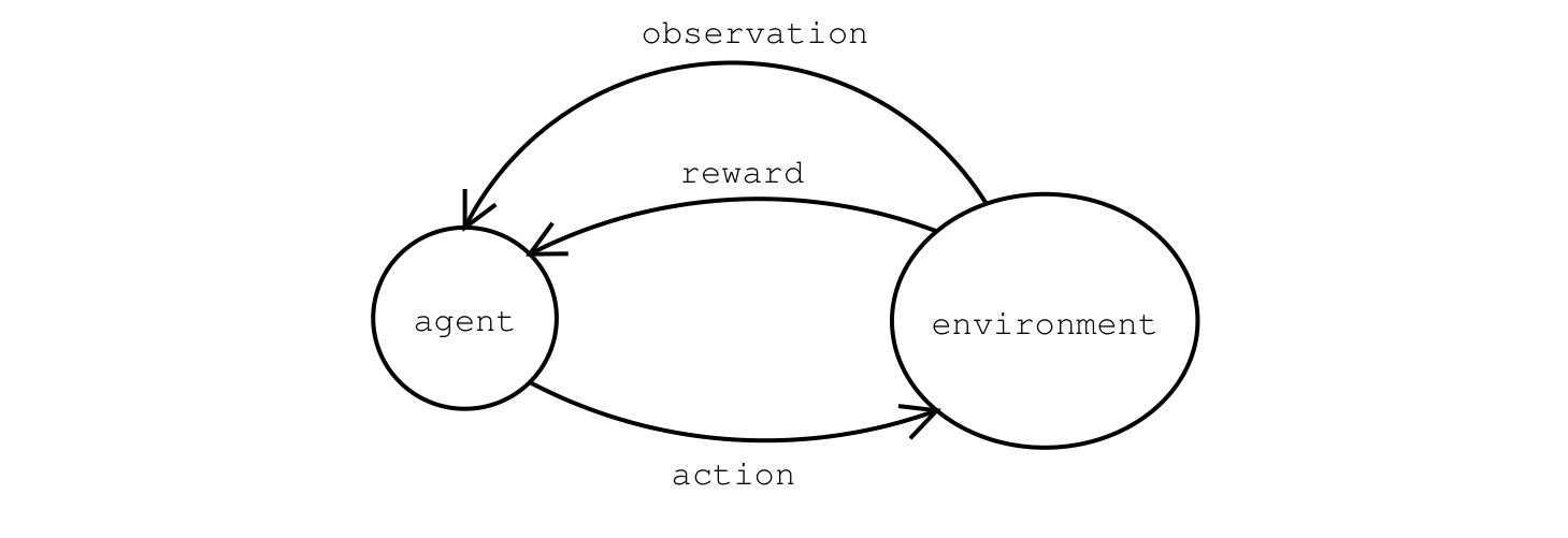
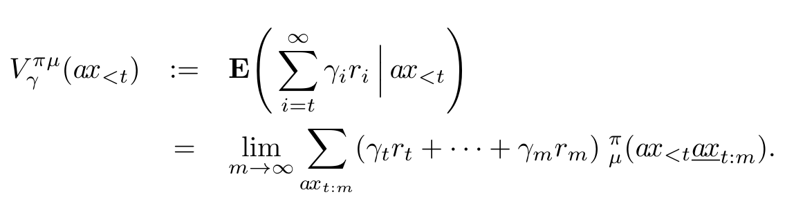
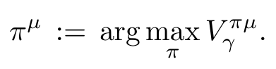
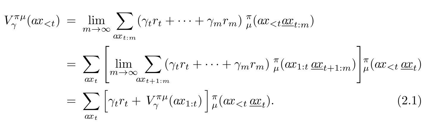
An interactive agent must also consider how actions affect future observations and rewards. AIXI combines a universal mixture over environments with sequential decision theory, selecting actions for expected future reward. The chapter develops the prior, agent–environment interaction, value functions, and optimality notions. Pareto optimality excludes uniform domination across environments. Self-optimization concerns asymptotic performance and requires appropriate environment classes; neither property guarantees quick learning or good behavior in every possible environment. [78, 155, 156]

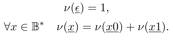
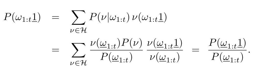
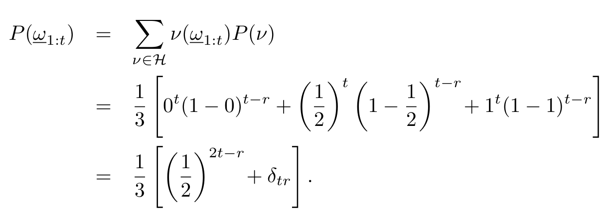
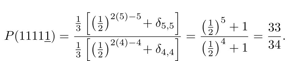
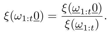
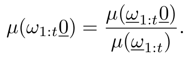
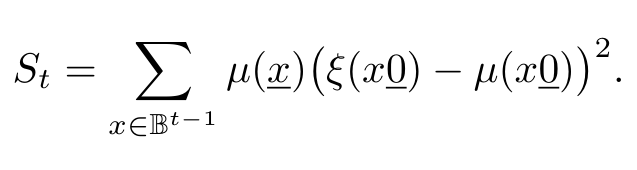
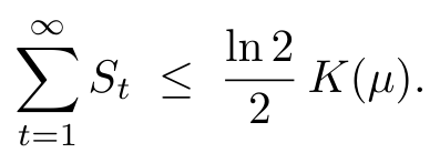
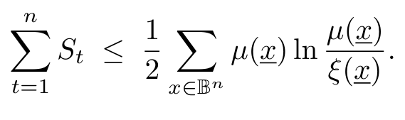
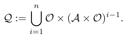
Equations p41-extra-15–p55-2
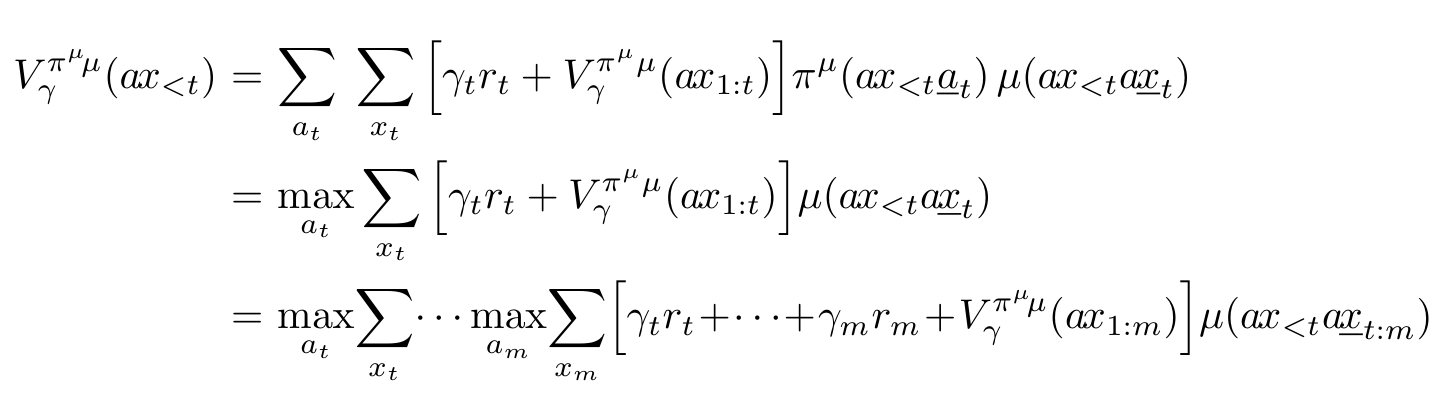
(p41-extra-15)Original displayed equation, PDF page 41
(p41-1)Original displayed equation, PDF page 41
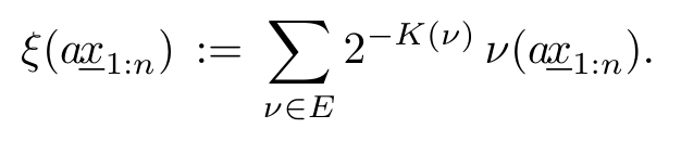
(p44-1)Original displayed equation, PDF page 44
(p44-2)Original displayed equation, PDF page 44
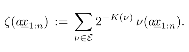
(p45-1)Original displayed equation, PDF page 45
(p45-2)Original displayed equation, PDF page 45
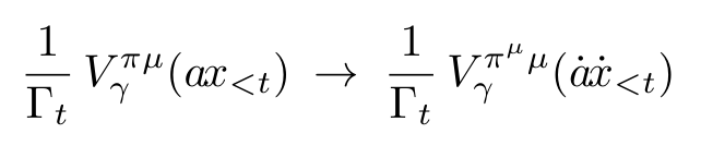
(p46-1)Original displayed equation, PDF page 46
(p46-2)Original displayed equation, PDF page 46
(p46-3)Original displayed equation, PDF page 46
(p47-1)Original displayed equation, PDF page 47
(p48-1)Original displayed equation, PDF page 48
(p49-1)Original displayed equation, PDF page 49
(p50-1)Original displayed equation, PDF page 50
(p50-2)Original displayed equation, PDF page 50
(p51-1)Original displayed equation, PDF page 51
(p53-1)Original displayed equation, PDF page 53
(p54-1)Original displayed equation, PDF page 54
(p54-2)Original displayed equation, PDF page 54
(p54-3)Original displayed equation, PDF page 54
(p54-4)Original displayed equation, PDF page 54
(p55-1)Original displayed equation, PDF page 55
(p55-2)Original displayed equation, PDF page 55
Figure 2.1.: The agent and the environment interact by sending action, observation and reward signals to each other.
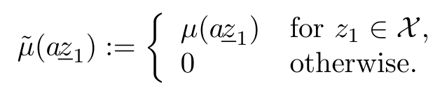
Equations p59-1–p66-1

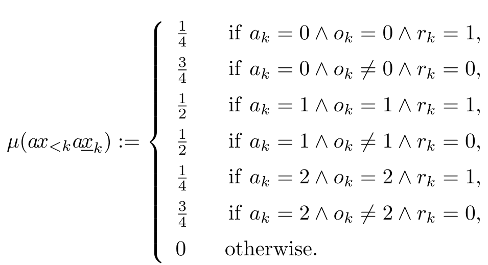
(p59-1)Original displayed equation, PDF page 59
(p59-2)Original displayed equation, PDF page 59
(p59-3)Original displayed equation, PDF page 59
(p60-1)Original displayed equation, PDF page 60
(p60-2)Original displayed equation, PDF page 60
(p61-1)Original displayed equation, PDF page 61
(p61-2)Original displayed equation, PDF page 61
(2.1)Original displayed equation, PDF page 61
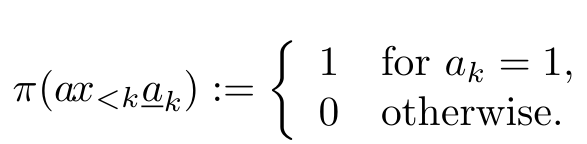
(p62-1)Original displayed equation, PDF page 62
(p62-2)Original displayed equation, PDF page 62
(p63-1)Original displayed equation, PDF page 63
(p64-1)Original displayed equation, PDF page 64
(p64-2)Original displayed equation, PDF page 64
(p65-1)Original displayed equation, PDF page 65
(p65-2)Original displayed equation, PDF page 65
(p66-1)Original displayed equation, PDF page 66
main(){while(1)printf("1");}

3. Taxonomy of Environments

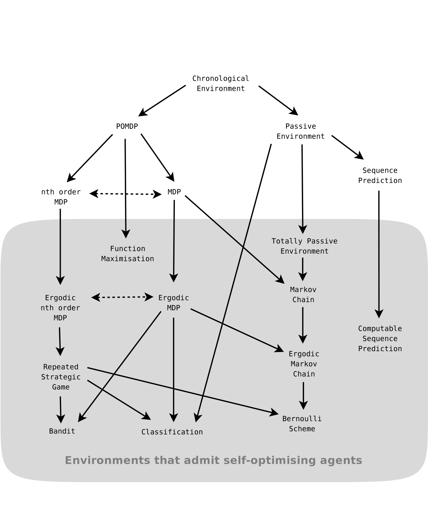
Where can optimal behavior be learned? The taxonomy separates passive processes from environments affected by actions, including Markov processes, MDPs, partially observed models, bandits, classification, repeated games, and sequence prediction. Some classes are special cases of others; others can be reduced by changing action and observation spaces.

The ergodic MDP argument supports self-optimization for several restricted classes. Unrestricted sequence prediction admits adversarial constructions, and universal-agent guarantees depend on the exact problem class and reward formulation. Even where a self-optimizing agent exists, convergence in the limit says nothing about whether its learning time is useful. The taxonomy figure distinguishes these relations and assumptions. [98, 78]

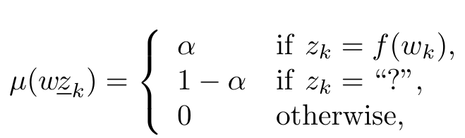
Equations p70-extra-1–p83-1

(p70-extra-1)Original displayed equation, PDF page 70
(p70-1)Original displayed equation, PDF page 70
(p70-2)Original displayed equation, PDF page 70
(p71-1)Original displayed equation, PDF page 71
(p71-2)Original displayed equation, PDF page 71
(p71-extra-2)Original displayed equation, PDF page 71
(p72-extra-3)Original displayed equation, PDF page 72
(p72-extra-4)Original displayed equation, PDF page 72
(p72-1)Original displayed equation, PDF page 72
(p72-2)Original displayed equation, PDF page 72
(p73-extra-5)Original displayed equation, PDF page 73
(p73-1)Original displayed equation, PDF page 73
(p73-extra-6)Original displayed equation, PDF page 73
(p74-1)Original displayed equation, PDF page 74
(p74-2)Original displayed equation, PDF page 74
(p74-extra-7)Original displayed equation, PDF page 74
(p75-1)Original displayed equation, PDF page 75
(p75-2)Original displayed equation, PDF page 75
(p75-3)Original displayed equation, PDF page 75
(p75-4)Original displayed equation, PDF page 75
(p76-1)Original displayed equation, PDF page 76
(p76-2)Original displayed equation, PDF page 76
(p77-extra-8)Original displayed equation, PDF page 77
(p77-1)Original displayed equation, PDF page 77
(p77-2)Original displayed equation, PDF page 77
(p78-1)Original displayed equation, PDF page 78
(p79-1)Original displayed equation, PDF page 79
(p80-1)Original displayed equation, PDF page 80
(3.1)Original displayed equation, PDF page 82
(p82-1)Original displayed equation, PDF page 82
(p83-1)Original displayed equation, PDF page 83
Figure 3.1.: Taxonomy of environments. Downward arrows indicate that the class below is a special case of the class above. Dotted horizontal lines indicate that two classes of environments are reducible to each other. The greyed area contains the classes of environments that admit self-optimising agents, that is, the environments in which a universal agent will learn to behave optimally.

4. Universal Intelligence Measure

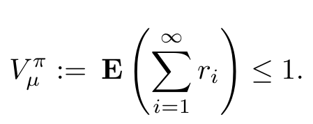
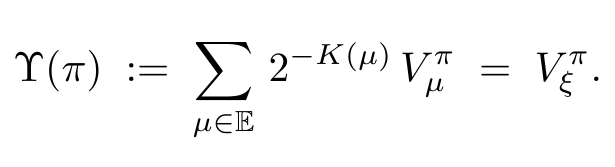
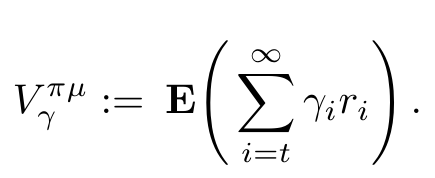
A proposed universal score. Measure an agent’s expected cumulative reward across computable, reward-summable environments, weighting each environment by a simplicity prior derived from Kolmogorov complexity. This turns the informal ambition of broad goal achievement into a precise mathematical quantity. The corresponding ideal Bayesian agent maximizes that quantity.

The score is incomputable and depends on the reference machine used to describe environments. Its broad coverage does not remove that choice. The chapter compares illustrative agents, evaluates desirable properties of intelligence measures, and responds to objections about computability, rewards, behavioral definitions, embodiment, and human-specific notions of understanding. These are arguments for a particular formalization, not empirical proof that one scalar captures every useful meaning of intelligence. Reward must remain specified by the task rather than freely set by the agent. [104]

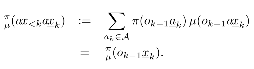
Equations p89-1–p96-1
(p89-1)Original displayed equation, PDF page 89
(p89-2)Original displayed equation, PDF page 89
(p93-1)Original displayed equation, PDF page 93
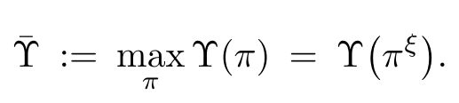
(p96-1)Original displayed equation, PDF page 96
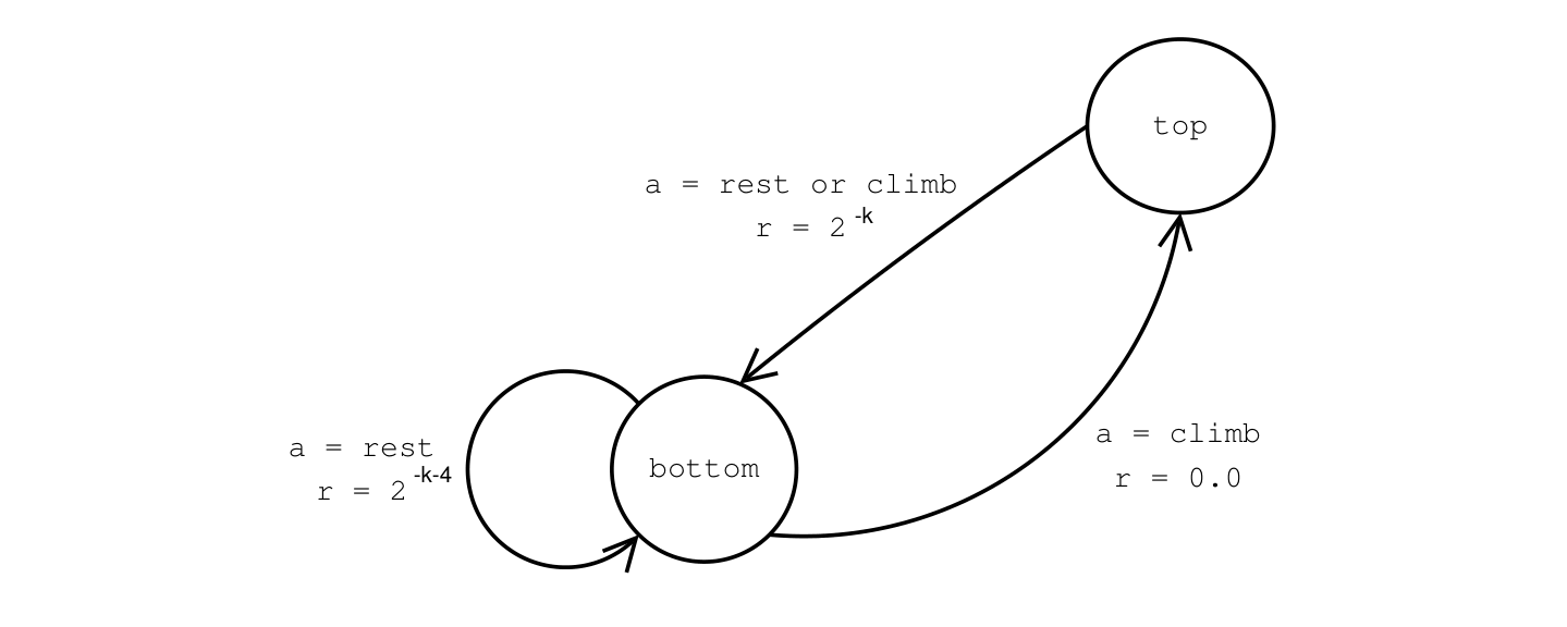
Figure 4.1.: A simple game in which the agent climbs a playground slide and slides back down again. A shortsighted agent will always just rest at the bottom of the slide.
Equation p98-1
(p98-1)Original displayed equation, PDF page 98
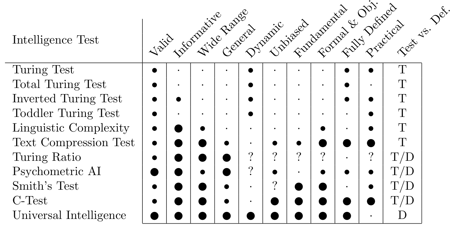
Table 4.1. A large filled dot means yes, a small filled dot means debatable, a point means no, and ? means unknown because the test is not sufficiently specified.

5. Limits of Computational Agents

Limits of computable prediction. For any computable predictor, a computable sequence can be constructed that defeats it. Predictors able eventually to predict every computable sequence below a description-length bound do exist, but their own descriptions must grow roughly with that bound. Some simple sequences are difficult to predict because generating them can require extreme computation.

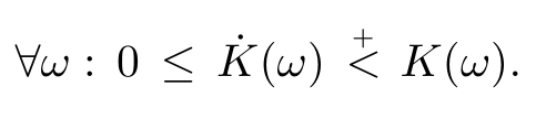
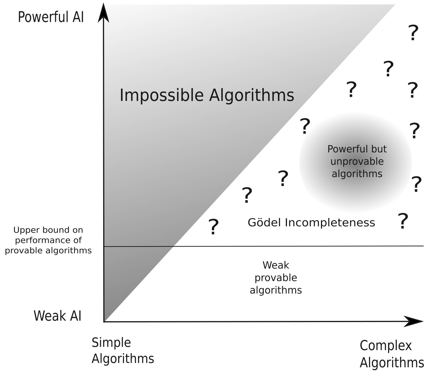
A further incompleteness result limits what a fixed sufficiently expressive, consistent formal system can prove about very powerful predictors. These are worst-case results about broad classes and eventual correctness, not evidence that practical learning on restricted data is impossible. The proposed direction is to constrain both environment generation and the learner’s resources, and to study learning speed as well as asymptotic success. [97]

Equations p114-1–p118-3

(p114-1)Original displayed equation, PDF page 114
(p118-1)Original displayed equation, PDF page 118
(p118-2)Original displayed equation, PDF page 118
(p118-3)Original displayed equation, PDF page 118
Figure 5.1.: Theorem 5.3.3 rules out simple but powerful artificial intelligence algorithms, as indicated by the greyed out region in the upper left. Theorem 5.6.1 upper bounds how powerful an algorithm can be before it can no longer be proven to be a powerful algorithm. This is indicated by the horizontal line separating the region of provable algorithms from the region of Gödel incompleteness.

6. Temporal Difference Updating without a Learning Rate

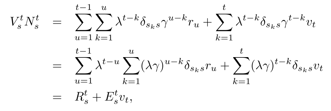
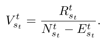
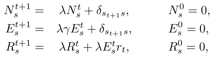
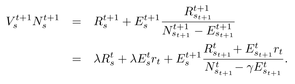
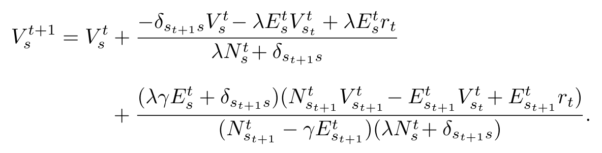
An empirical learning rule. Starting from a squared-error objective for state values, the derivation replaces TD(λ)’s manually chosen learning rate with a transition-dependent expression involving visit counts and eligibility traces. The resulting HL(λ) rule still requires other choices, including discounting and the treatment of old observations. It is not parameter-free.

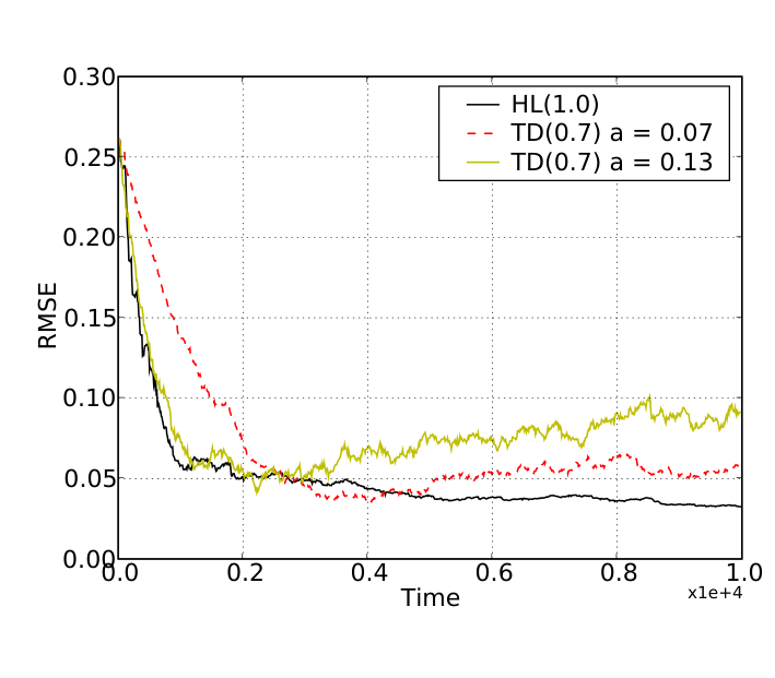
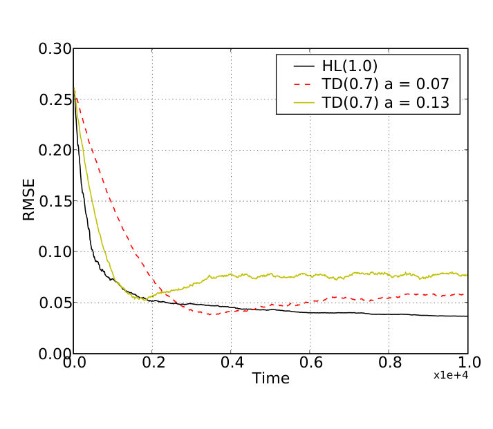
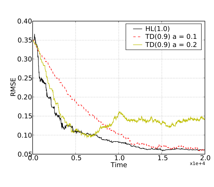
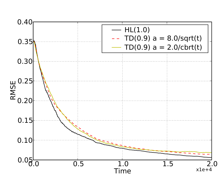
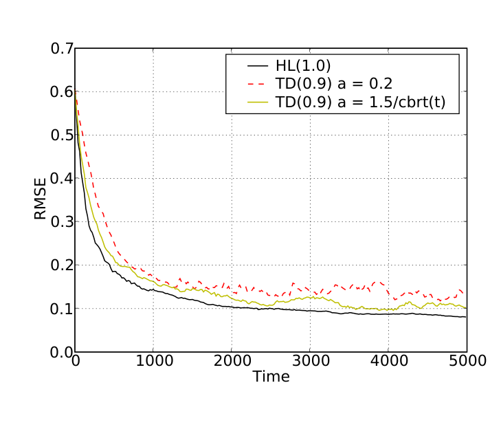
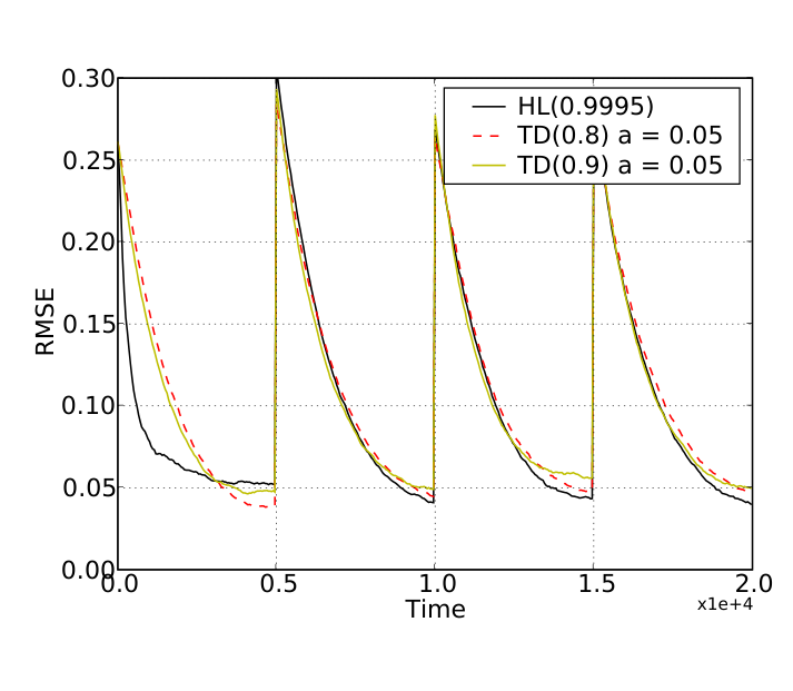
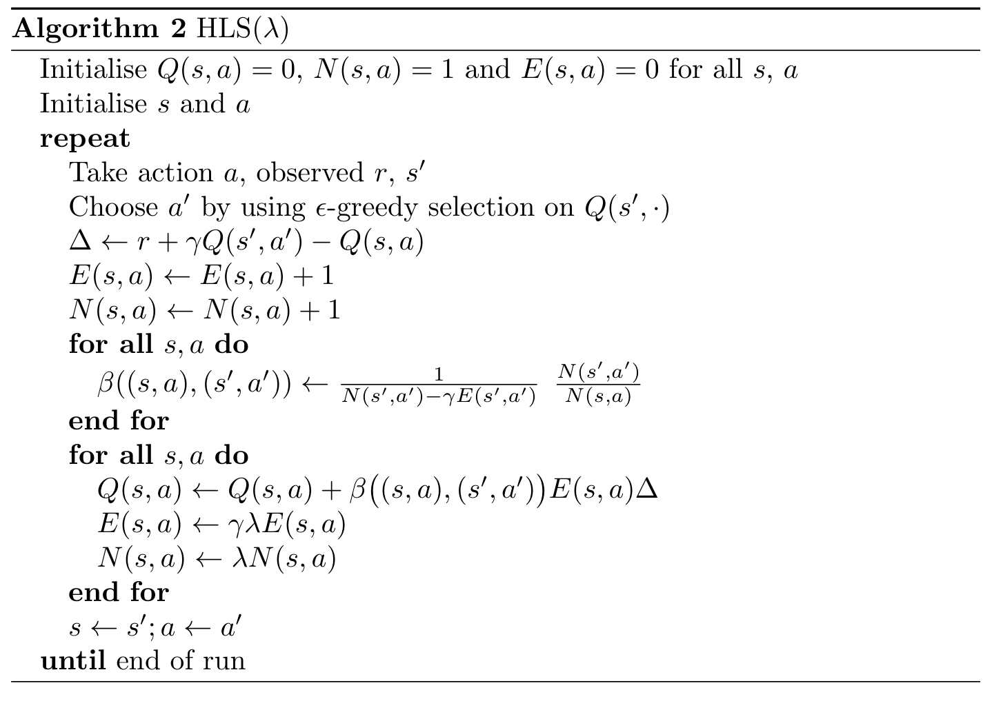
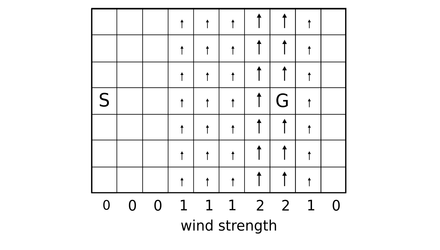
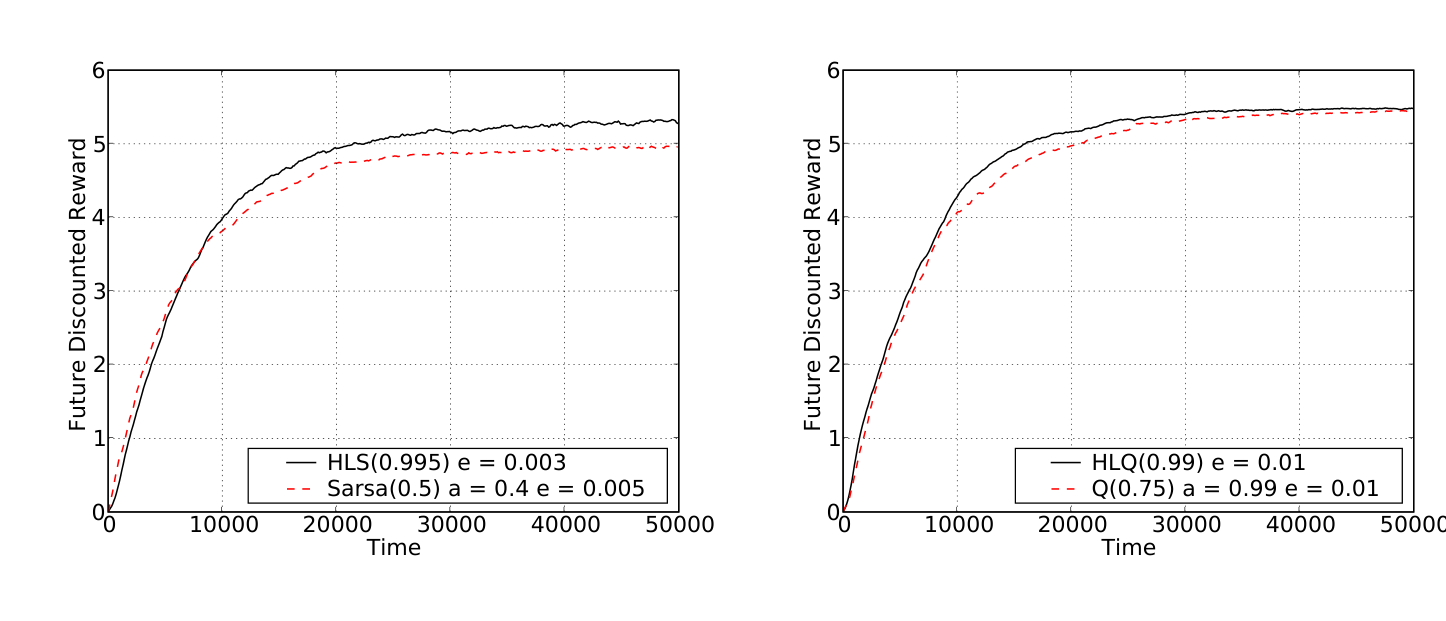
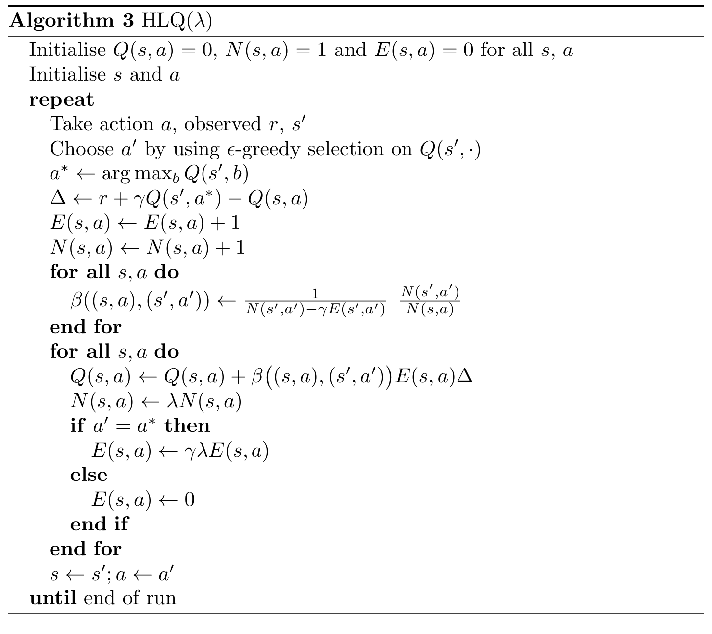
Experiments cover 21-state and 51-state random walks, a random 50-state Markov process, changing rewards, and a continuing Windy Gridworld. In the reported comparisons, HL updates improve learning or final value estimates relative to the tuned TD baselines. The reinforcement-learning variants HLS and HLQ replace updates in Sarsa and Watkins’ Q-learning; HLS costs about 1.7 times as much per step as the compared Sarsa implementation. The nonstationary experiment also reveals a tradeoff between rapid adaptation and final accuracy.

All eight experimental figures and three algorithms are retained. The evidence is limited to these small tabular settings. Convergence proofs, episodic extensions, broader tasks, and function approximation are left for future work; the reported success does not establish general superiority. [83, 164, 165, 179]

Equations p126-1–p126-3

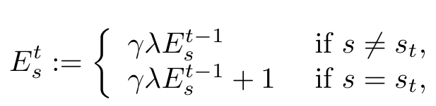
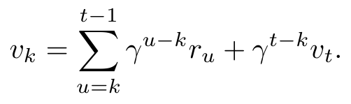
(p126-1)Original displayed equation, PDF page 126
(6.1)Original displayed equation, PDF page 126
(p126-3)Original displayed equation, PDF page 126
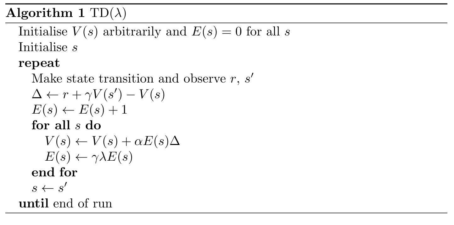
Algorithm 1. TD(λ).
Algorithm 1. TD(λ).
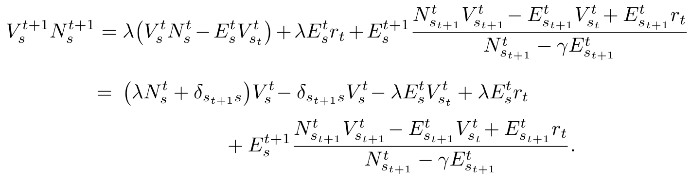
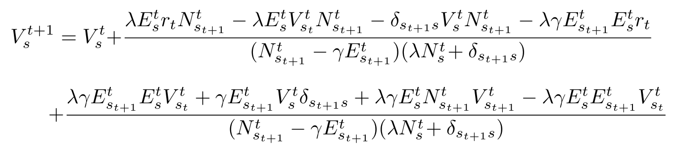
Equations p127-1–6.9
(p127-1)Original displayed equation, PDF page 127
(6.2)Original displayed equation, PDF page 127
(6.3)Original displayed equation, PDF page 128
(6.4)Original displayed equation, PDF page 128
(p129-1)Original displayed equation, PDF page 129
(6.5)Original displayed equation, PDF page 129
(p129-3)Original displayed equation, PDF page 129
(p129-4)Original displayed equation, PDF page 129
(6.6)Original displayed equation, PDF page 129
(p129-6)Original displayed equation, PDF page 129
(6.7)Original displayed equation, PDF page 130
(p130-2)Original displayed equation, PDF page 130
(p130-3)Original displayed equation, PDF page 130
(p130-4)Original displayed equation, PDF page 130
(p130-5)Original displayed equation, PDF page 130
(p130-6)Original displayed equation, PDF page 130
(p131-1)Original displayed equation, PDF page 131
(p131-2)Original displayed equation, PDF page 131
(6.8)Original displayed equation, PDF page 131
(6.9)Original displayed equation, PDF page 131
Figure 6.1.: 21 state Markov process, average performance over 10 runs.
Figure 6.2.: 21 state Markov process, average performance over 100 runs.
Figure 6.3.: 51 state Markov process averaged over 10 runs. The parameter a is the learning rate α.
Figure 6.4.: 51 state Markov process averaged over 300 runs.
Figure 6.5.: Random 50 state Markov process. The parameter a is the learning rate α.
Figure 6.6.: 21 state non-stationary Markov process.
Algorithm 2. HLS(λ).
Figure 6.7.: [Windy Gridworld] S marks the start state and G the goal state, at which the agent jumps back to S with a reward of 1. Small arrows indicate an upward wind of one row per time step. The large arrows indicate a wind of two rows per time step.
Figure 6.8.: Windy Gridworld performance tests. The left graph shows HLS(λ) vs. Sarsa(λ), while the right graph shows HLQ(λ) vs. Q(λ). In both tests the algorithm based on HL learning performed best. e represents the exploration parameter ǫ, and a represents the learning rate α. For both tests the performance was averaged over 500 runs.
Algorithm 3. HLQ(λ).

7. Discussion

Implications in 2008. The discussion considers whether powerful general machines are possible and examines theoretical design, biological inspiration, and artificial evolution as research paths. Formal ideals can organize questions without supplying a practical construction. Evolutionary approaches also depend on useful fitness functions, representations, diversity, and computational resources.

Legg argues that the potential benefits and hazards justify studying safe goal specification before very powerful systems arrive. This is a forward-looking discussion from the dissertation’s time, not an experimental result or a current forecast. The thesis provides neither a demonstrated superintelligent machine nor a guarantee that maximizing a specified reward produces desirable real-world behavior. [51]

Appendix A. Notation and Conventions

The notation guide defines equality and approximation conventions, sets and intervals, binary strings and sequences, probability notation, algorithms, and additive or multiplicative comparisons of complexity. Its role is to make the mathematical assumptions in the chapters precise; unnumbered preserved equations are labeled by their PDF page and order in this edition.

Appendix B. Ergodic MDPs Admit Self-optimising Agents

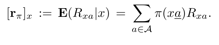
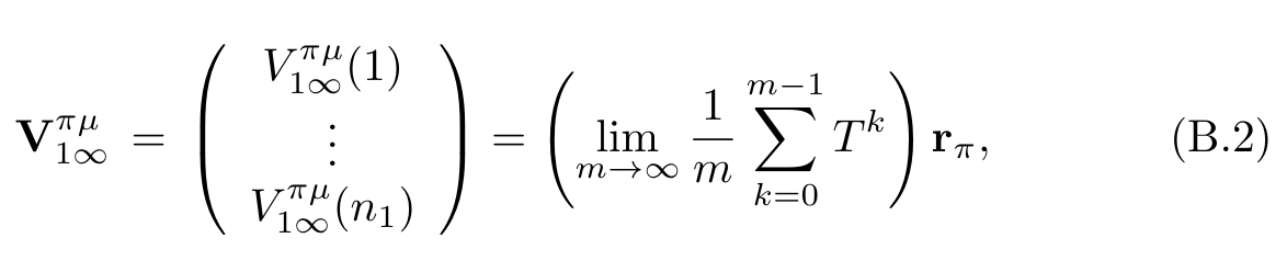
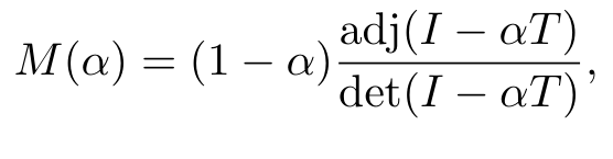
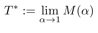
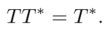
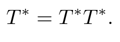
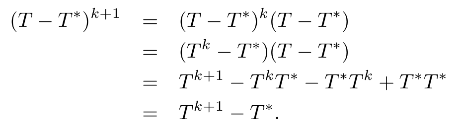
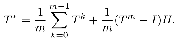
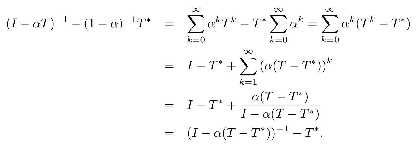
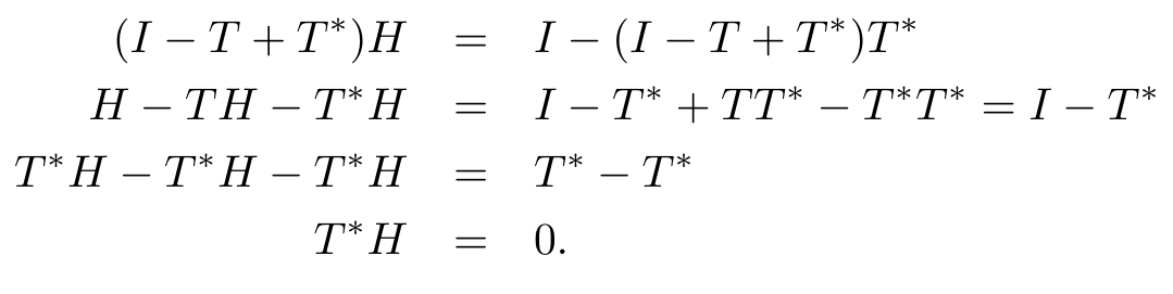
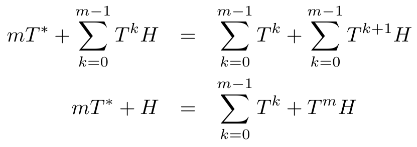
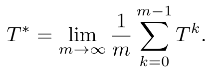
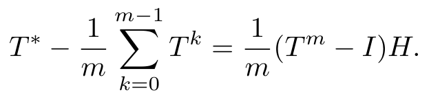
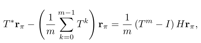
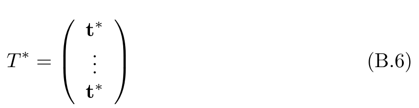
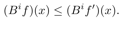
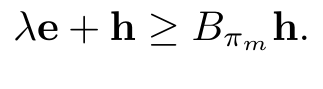
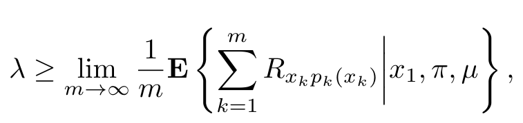
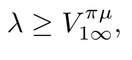
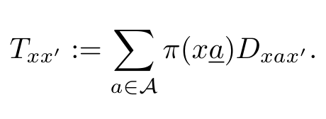
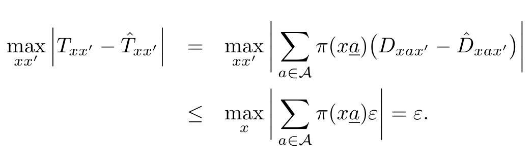
The proof formalizes stationary policies, transition matrices, reward vectors, and long-run average value in a finite ergodic MDP. It analyzes the limiting behavior of stationary Markov chains, establishes the existence of an optimal stationary policy, and controls the effect of estimated transition probabilities.

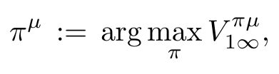
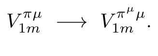
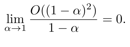
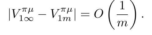
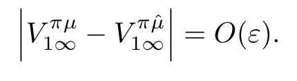
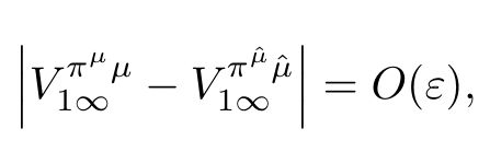
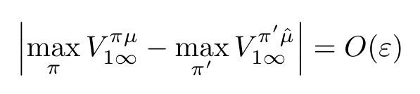
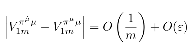
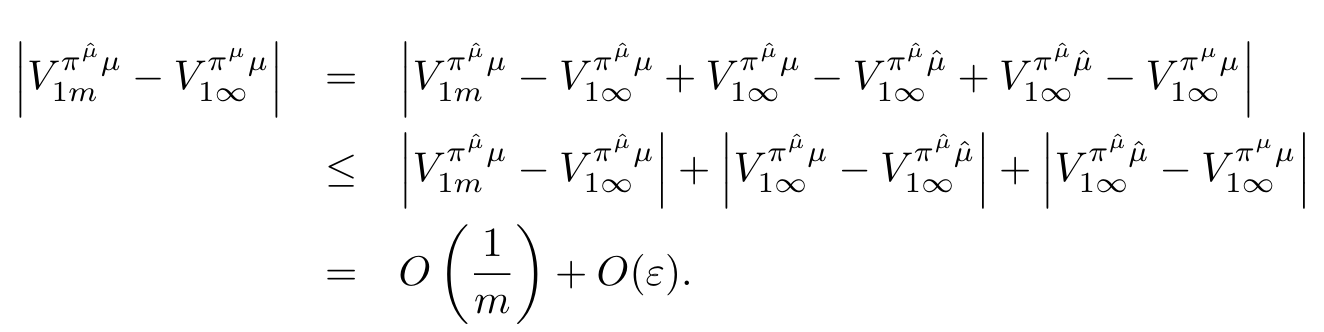
An agent can spend an initial period gathering data and then exploit a policy optimized for its estimated model. With an appropriate balance, estimation error and the fraction of time spent exploring vanish, yielding convergence of expected average value. The conclusion depends on the appendix’s ergodicity and finite-state assumptions and is asymptotic. The complete displayed derivation is retained for inspection. [12, 78]

Equations p160-extra-9–p173-3

(p160-extra-9)Original displayed equation, PDF page 160
(p160-1)Original displayed equation, PDF page 160
(B.1)Original displayed equation, PDF page 160
(p160-3)Original displayed equation, PDF page 160
(p161-1)Original displayed equation, PDF page 161
(p161-2)Original displayed equation, PDF page 161
(B.2)Original displayed equation, PDF page 161
(p161-4)Original displayed equation, PDF page 161
(p162-1)Original displayed equation, PDF page 162
(p162-2)Original displayed equation, PDF page 162
(p162-3)Original displayed equation, PDF page 162
(p162-4)Original displayed equation, PDF page 162
(p162-5)Original displayed equation, PDF page 162
(p163-1)Original displayed equation, PDF page 163

(p163-2)Original displayed equation, PDF page 163
(B.3)Original displayed equation, PDF page 163
(p163-4)Original displayed equation, PDF page 163
(p163-5)Original displayed equation, PDF page 163
(p163-6)Original displayed equation, PDF page 163
(p163-7)Original displayed equation, PDF page 163
(p163-8)Original displayed equation, PDF page 163
(p164-1)Original displayed equation, PDF page 164
(p164-2)Original displayed equation, PDF page 164
(p164-3)Original displayed equation, PDF page 164
(p164-4)Original displayed equation, PDF page 164
(p164-5)Original displayed equation, PDF page 164
(p164-6)Original displayed equation, PDF page 164
(p164-7)Original displayed equation, PDF page 164
(p164-8)Original displayed equation, PDF page 164
(p164-9)Original displayed equation, PDF page 164
(p165-1)Original displayed equation, PDF page 165
(B.4)Original displayed equation, PDF page 165
(p165-3)Original displayed equation, PDF page 165
(p165-4)Original displayed equation, PDF page 165
(p165-5)Original displayed equation, PDF page 165
(p165-6)Original displayed equation, PDF page 165
(p165-7)Original displayed equation, PDF page 165
(p166-1)Original displayed equation, PDF page 166
(B.5)Original displayed equation, PDF page 166
(p166-3)Original displayed equation, PDF page 166
(p166-4)Original displayed equation, PDF page 166
(p166-5)Original displayed equation, PDF page 166
(B.6)Original displayed equation, PDF page 167
(p167-extra-10)Original displayed equation, PDF page 167
(p167-extra-11)Original displayed equation, PDF page 167
(p167-extra-12)Original displayed equation, PDF page 167
(p167-3)Original displayed equation, PDF page 167
(p168-2)Original displayed equation, PDF page 168
(p168-3)Original displayed equation, PDF page 168
(p169-1)Original displayed equation, PDF page 169
(p169-extra-13)Original displayed equation, PDF page 169
(B.7)Original displayed equation, PDF page 169
(p169-3)Original displayed equation, PDF page 169
(p169-4)Original displayed equation, PDF page 169
(p169-5)Original displayed equation, PDF page 169
(p169-6)Original displayed equation, PDF page 169
(p170-1)Original displayed equation, PDF page 170
(p170-2)Original displayed equation, PDF page 170
(p170-3)Original displayed equation, PDF page 170
(p170-4)Original displayed equation, PDF page 170
(p170-5)Original displayed equation, PDF page 170
(B.8)Original displayed equation, PDF page 170
(p170-7)Original displayed equation, PDF page 170
(p170-8)Original displayed equation, PDF page 170
(p171-2)Original displayed equation, PDF page 171
(p172-1)Original displayed equation, PDF page 172
(p172-2)Original displayed equation, PDF page 172
(B.9)Original displayed equation, PDF page 172
(p172-4)Original displayed equation, PDF page 172
(p172-5)Original displayed equation, PDF page 172
(p173-1)Original displayed equation, PDF page 173
(p173-2)Original displayed equation, PDF page 173
(p173-3)Original displayed equation, PDF page 173

Appendix C. Definitions of Intelligence

The collection gathers definitions from reference works, psychologists, and artificial-intelligence researchers. Recurrent themes include learning, reasoning, adaptation, problem solving, and effective goal pursuit, but the definitions emphasize different abilities and contexts. The appendix is historical supporting material for the thesis’s chosen definition, not a claim that all authors endorse the later universal intelligence formula. [102]

Concept demonstration

Open image ↗