At a glance
The dissertation treats concepts as typed combinations of symbolic programs and learned neural representations. Object properties, relations and actions are grounded in perception or control, then composed for visual reasoning and planning. Its three parts develop logic and constraint-solving foundations, visual concept learning, and robot skill/planning representations.
The evidence spans distinct models and benchmark studies. Reported data efficiency and compositional transfer depend on each chapter’s supervision, representation and evaluation assumptions; the dissertation does not demonstrate a single deployed lifelong generalist agent. This edition retains the original figures, tables, mathematical displays, algorithms, code and prompts, including all thirteen appendices.
The source was submitted on September 12, 2025; its title page states February 2026.
Prologue: Concepts
The central proposal is to learn an abstract world model and reason with it at performance time. Concepts provide reusable units rather than requiring a separate end-to-end predictor for every task. Abstraction shares knowledge across instances; composition builds new descriptions and plans from known pieces.
Physical experience and language supply complementary information. This is a research program supported by the later chapters’ individual systems, rather than an empirical claim that all forms of intelligence reduce to one demonstrated architecture.
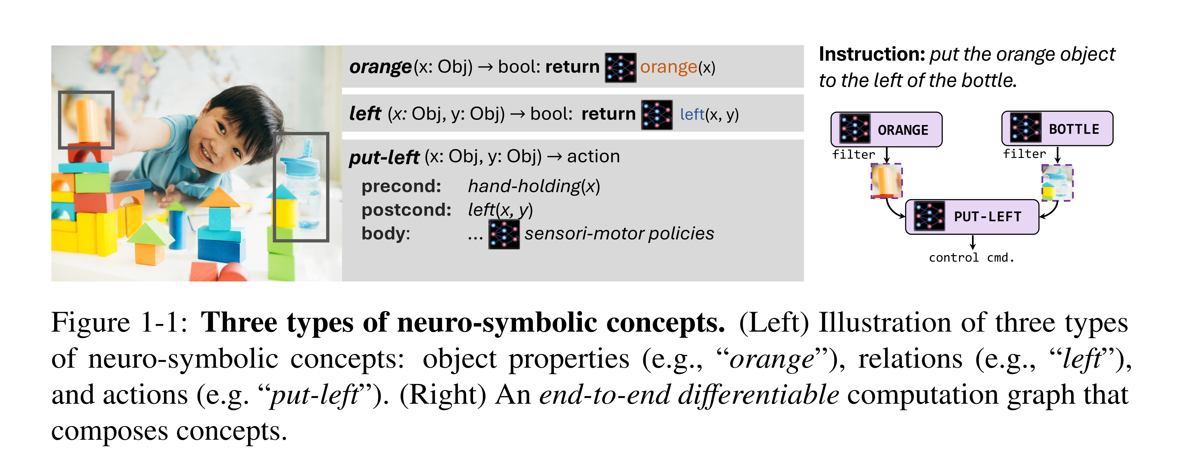
Figure 1-1: Three types of neuro-symbolic concepts. (Left) Illustration of three types of neuro-symbolic concepts: object properties (e.g., “orange”), relations (e.g., “left”), and actions (e.g. “put-left”). (Right) An end-to-end differentiable computation graph that composes concepts.
Neuro-Symbolic Concepts
A concept is a tuple of parameters, a program and neural-network components. A property such as orange grounds a symbol in object features; a relation such as left-of scores object pairs. An action additionally specifies a controller and pre-/postconditions. Typed inputs and outputs constrain valid compositions.
The symbolic part specifies how computations combine, while learned components ground their meaning in observations or actuation. The original tuple definitions and both figures are retained. The choice of primitive operations and grounding architecture remains domain-dependent.
Equations



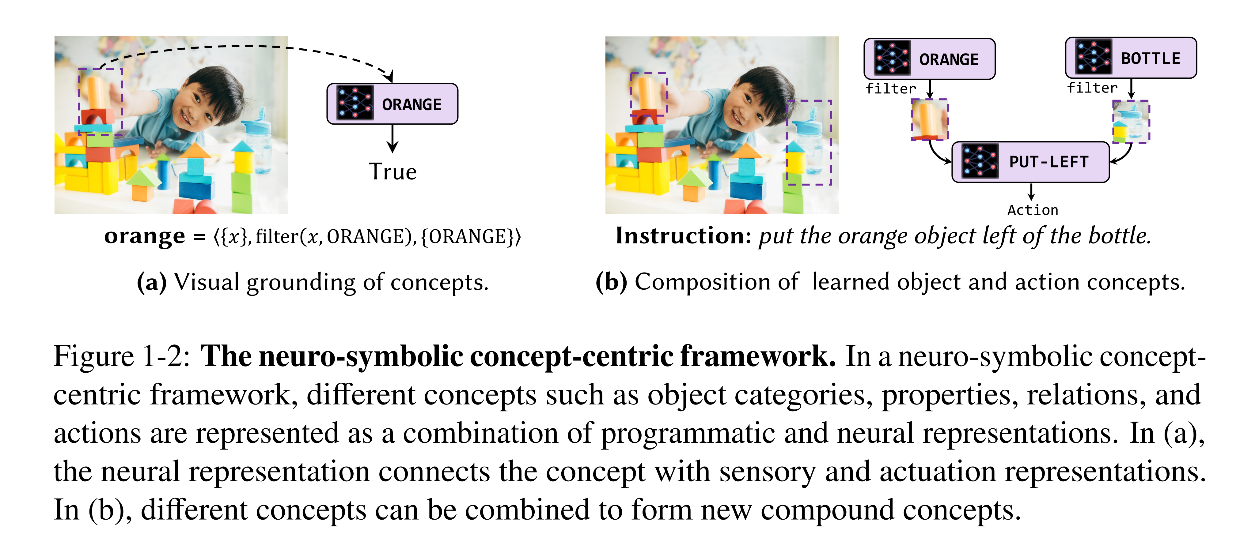
Figure 1-2: The neuro-symbolic concept-centric framework. In a neuro-symbolic concept- centric framework, different concepts such as object categories, properties, relations, and actions are represented as a combination of programmatic and neural representations. In (a), the neural representation connects the concept with sensory and actuation representations. In (b), different concepts can be combined to form new compound concepts.
Equation

Structure of the Dissertation
Part I develops Neural Logic Machines, temporal/object quantification, expressiveness and planning-complexity results, and compositional diffusion constraint solvers. Part II studies joint vision/language concept learning, fast learning through metaconcepts, cross-domain grounding and lexicon acquisition.
Part III builds manipulation mechanisms, planning-compatible learned action models, and hybrid imperative–declarative programs. The theory gives conditional bounds and the experiments establish specific capabilities; neither should be generalized beyond the stated problem class, supervision or resource budget. The final chapters identify the further integration, memory, uncertainty and human-interaction work needed for a complete agent.
I Foundations of Neuro-Symbolic Representation and Reasoning
Part I develops reusable neuro-symbolic representations for relational, temporal, planning, and continuous-constraint problems. Its recurring design principle is to encode compositional structure explicitly while learning the local functions that operate on it. The chapters separate architectural expressiveness from the practical questions of training, computational cost, and generalization.
Neuro-Symbolic First-Order Logic
This chapter combines Neural Logic Machines with the later SpaLoc framework. NLM learns shared computations over object tuples and quantifiers; SpaLoc adds sparse intermediate representations and local subgraph training to make higher-order reasoning practical on larger graphs. The two experimental settings and their scalability claims should be read separately.
Introduction
Blocks-world planning motivates four requirements: transfer across object counts, reasoning about more than pairs of objects, composing many intermediate predicates, and reducing reliance on hand-written rule templates. NLM uses shared neural transformations and quantifier wiring to meet these architectural goals. The demonstrated learner still receives structured predicates, chosen depth and arity, curriculum, and task-specific training support; absence of supplied rules does not mean absence of inductive bias.
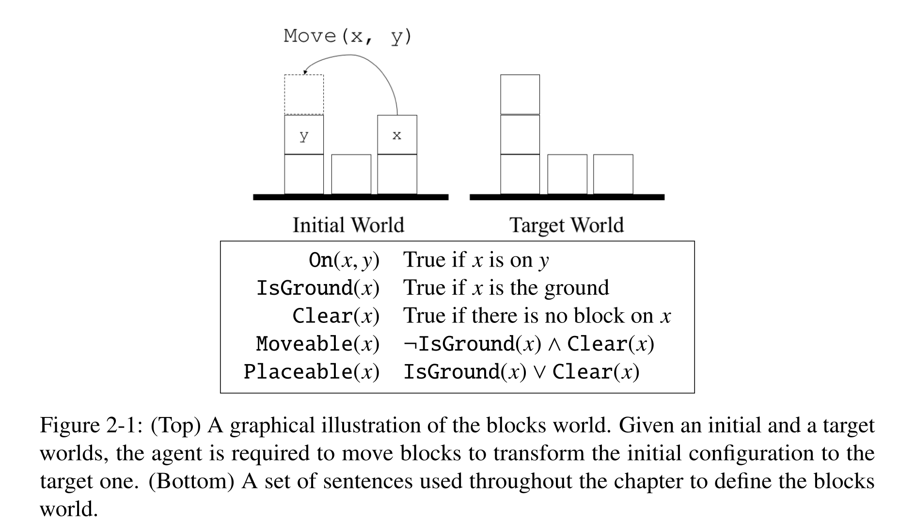
Figure 2-1: (Top) A graphical illustration of the blocks world. Given an initial and a target worlds, the agent is required to move blocks to transform the initial configuration to the target one. (Bottom) A set of sentences used throughout the chapter to define the blocks world.
Neural Logic Machines (NLM)
Under a finite-domain, closed-world formulation, predicates become tensors of grounded truth scores. Layers transform these tensors into new properties and relations. Neural functions supply soft Boolean computation, while fixed expansion, reduction, and permutation operations express the structure of quantified reasoning.
Logic Predicates as Tensors
An arity-r predicate has one entry for each ordered tuple of distinct objects; repeated-argument cases can be represented with lower-arity predicates. Channels hold multiple predicates, and arity zero stores global properties. Scores in [0,1] permit gradient-based training. Maximum arity is the architecture’s breadth. Arguments are variables or object constants, without function symbols. Parameter sharing supports different object counts, although tensor size still grows with the number of tuples.
Logic Rules as Neural Operators
A shared perceptron receives all permutations of a tuple’s predicate features and produces soft derived predicates. Expansion repeats a lower-arity feature over an added variable; reduction uses maximum and minimum over a removed variable to implement existential and universal quantification on Boolean inputs. The ValidMove and Moveable examples demonstrate how differently scoped predicates can be aligned and combined. These operations define the logical relaxation; learned intermediate scores need not be calibrated probabilities.
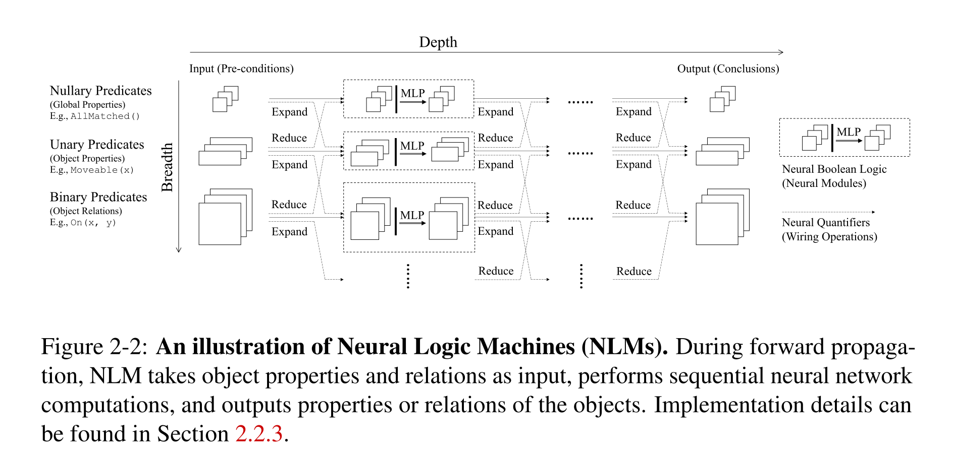
Figure 2-2: An illustration of Neural Logic Machines (NLMs). During forward propaga- tion, NLM takes object properties and relations as input, performs sequential neural network computations, and outputs properties or relations of the objects. Implementation details can be found in Section 2.2.3.
Equations








Neural Logic Machines
Each layer combines same-arity features with expanded lower-arity and reduced higher-arity features, then permutes arguments and applies a shared neural transformation. All arity groups read the previous layer, with missing neighbors omitted at the boundaries. The construction supports finite-depth forward chaining with sufficient channels and breadth. Cyclic predicate dependencies are deferred, so this is not an unrestricted recursive logic engine.
Equation

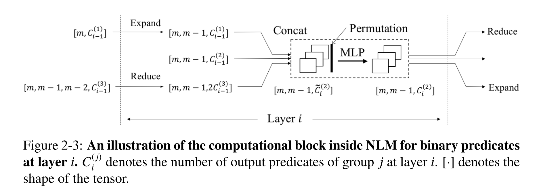
Figure 2-3: An illustration of the computational block inside NLM for binary predicates at layer i. C( j) i denotes the number of output predicates of group j at layer i. [·] denotes the shape of the tensor.
Equation

Expressiveness and Computational Complexity
Depth limits deduction steps, breadth limits tuple arity, channels limit intermediate predicates, and perceptron capacity limits the local Boolean computation. With breadth treated as a small constant, the stated cost is O(mᴮDC²) and the parameter count O(DC²). The omitted breadth-dependent constants include factorial argument permutations. Object-count-independent parameters therefore coexist with rapidly growing computation and memory.
Experiments
Family and graph tasks use supervised predicate labels; blocks world, sorting, and path finding use reinforcement learning. Training occurs on smaller instances and testing on larger object sets. Appendix A supplies the curriculum, model-selection criteria, auxiliary objectives, and graduation rates needed to interpret the headline test accuracies.
Baselines
Memory Networks encode object identifiers and relation values as queryable memory entries. Differentiable ILP uses grounded base predicates. Additional DNC and graph-network results are cited from related task formulations. Differences in querying, output formulation, and supervision limit direct interpretation of those additional comparisons.
Family Tree Reasoning
Training uses twenty-person synthetic families; tests use twenty or one hundred people. Targets include parent existence, sisters, grandparents, uncles, and maternal great uncles. NLM and differentiable ILP achieve 100% in Table 2.1, whereas the Memory Network often degrades on larger families. Its paired entries are micro and macro accuracy. The cited DNC number concerns finding a relative, not classifying every object pair. Appendix A’s graduation rates qualify how consistently these successful models are obtained.
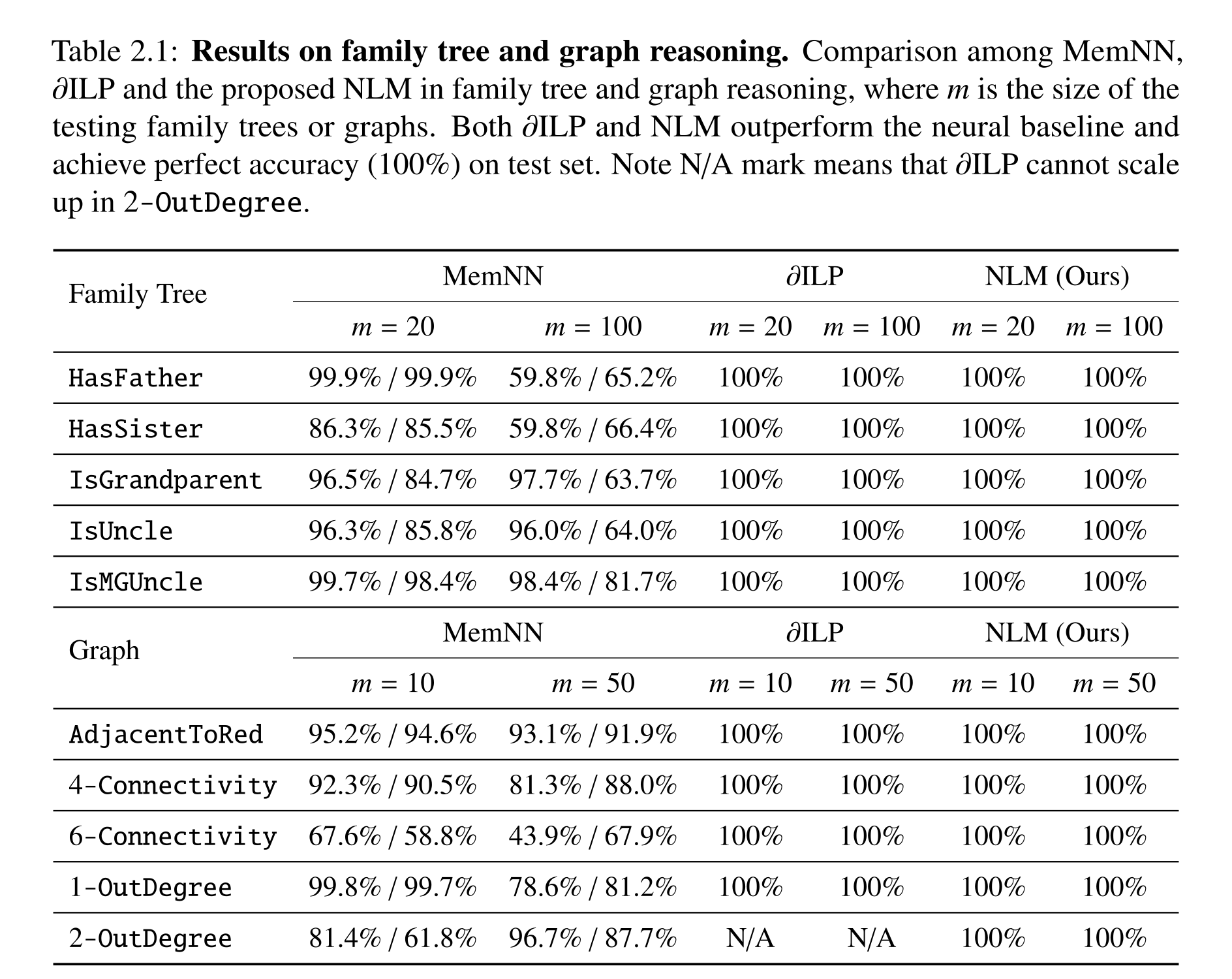
Table 2.1: Results on family tree and graph reasoning. Comparison among MemNN, ∂ILP and the proposed NLM in family tree and graph reasoning, where m is the size of the testing family trees or graphs. Both ∂ILP and NLM outperform the neural baseline and achieve perfect accuracy (100%) on test set. Note N/A mark means that ∂ILP cannot scale up in 2-OutDegree.
General Graph Reasoning
Ten-node training graphs and ten- or fifty-node tests supply adjacency and node colors. Tasks concern adjacency to a red node, bounded-distance connectivity, and exact out-degree. NLM reaches 100% on the reported tests. Differentiable ILP’s missing two-out-degree result reflects its memory limit on the required higher-arity computation, rather than an inability of logic itself to express the property.
Blocks World
The policy compares identities and coordinates across current and target block configurations and selects pairwise move actions. Invalid moves leave the state unchanged. Reported NLM success is 100% on sampled ten- and fifty-block cases, with twelve and eighty-four moves on average; Memory Networks fail within the stated limit. Appendix A.2.5 clarifies that the action head joins current and target representations by identity and receives supervised action-validity/effect training in addition to reinforcement learning.
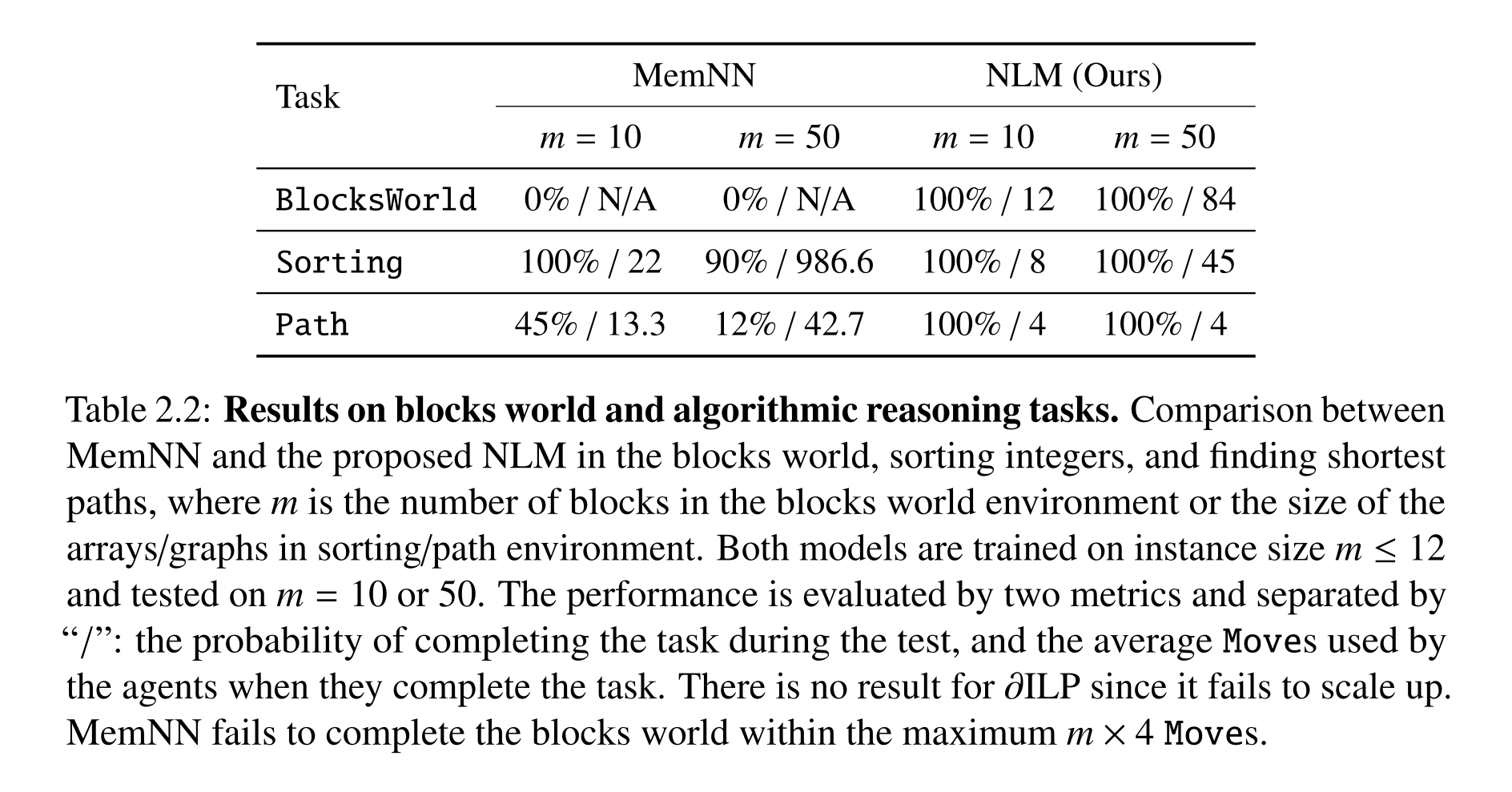
Table 2.2: Results on blocks world and algorithmic reasoning tasks. Comparison between MemNN and the proposed NLM in the blocks world, sorting integers, and finding shortest paths, where m is the number of blocks in the blocks world environment or the size of the arrays/graphs in sorting/path environment. Both models are trained on instance size m ≤12 and tested on m = 10 or 50. The performance is evaluated by two metrics and separated by “/”: the probability of completing the task during the test, and the average Moves used by the agents when they complete the task. There is no result for ∂ILP since it fails to scale up. MemNN fails to complete the blocks world within the maximum m × 4 Moves.
General Algorithms
Sorting supplies every pairwise index and value comparison and learns a swap policy; the larger fifty-element test takes forty-five swaps on average. Path finding moves a marked current node toward a target. Although graph size grows, training path distances are at most five and testing distance is four, so perfect four-step results do not demonstrate transfer to arbitrarily long paths. Learned behaviors resemble familiar algorithms, but the experiment does not extract and prove a universally correct symbolic program.
Sparsity and Locality in Neural Logic Machines
Dense higher-order tensors become prohibitive on large graphs. SpaLoc exploits two empirical properties of relational reasoning: useful intermediate relations are often sparse, and a prediction often depends on a small local set of entities. It combines sparse coordinate-list tensors, learned gates regularized for sparsity, and subgraph training with adjusted labels. Sparsity and locality are learned or approximated assumptions, not guarantees that every relational task has a cheap local solution.
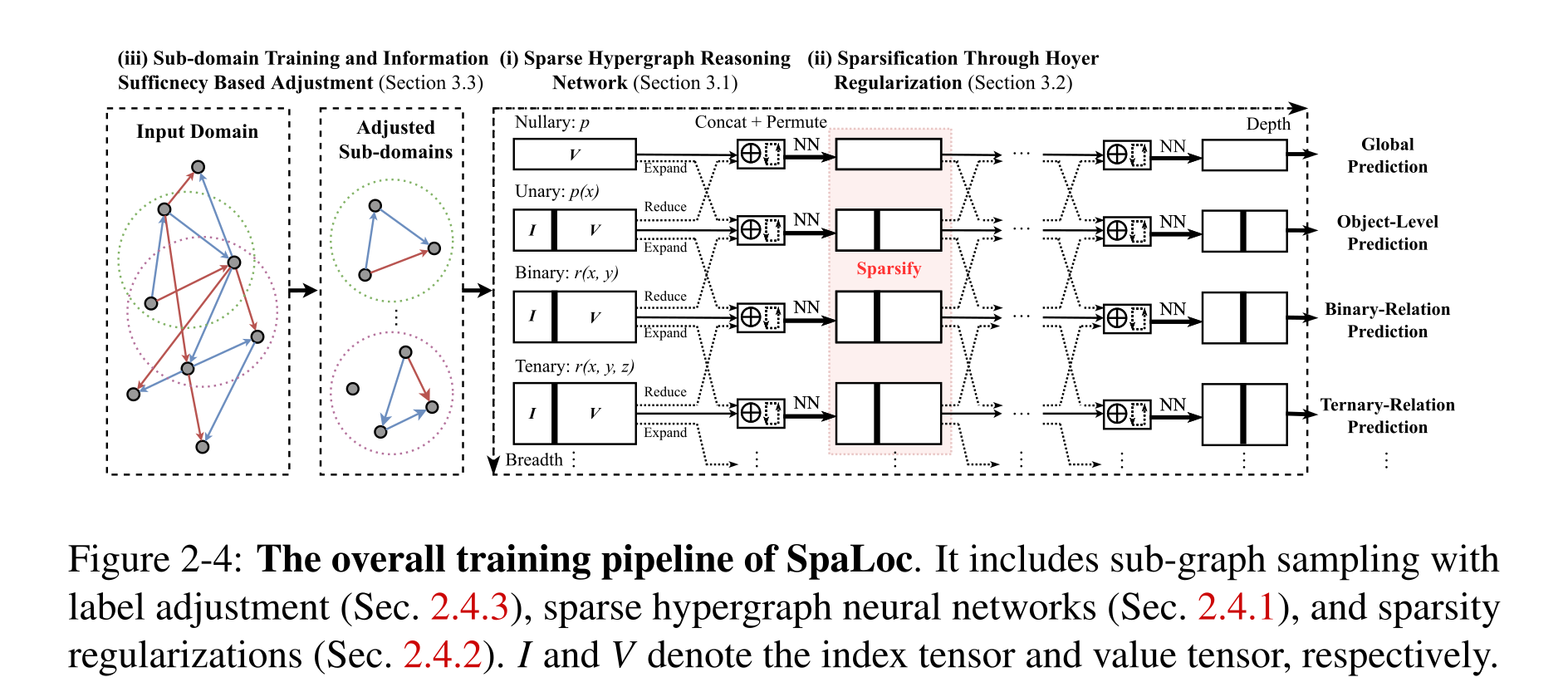
Figure 2-4: The overall training pipeline of SpaLoc. It includes sub-graph sampling with label adjustment (Sec. 2.4.3), sparse hypergraph neural networks (Sec. 2.4.1), and sparsity regularizations (Sec. 2.4.2). I and V denote the index tensor and value tensor, respectively.
Sparse Hypergraph Neural Networks
Sparse tensors store explicit tuple indices and feature values, treating unlisted tuples as zero. Expansion, max reduction, union-and-padding concatenation, and argument permutation generalize NLM operations to this representation. A learned scalar gate multiplies every channel of a tuple; inference prunes gates below 0.05. Intermediate sparsity is not known beforehand, so training still needs local dense computation and regularization. Expansion and permutation can create new entries. Higher arity improves representational power but retains its intrinsic combinatorial cost.
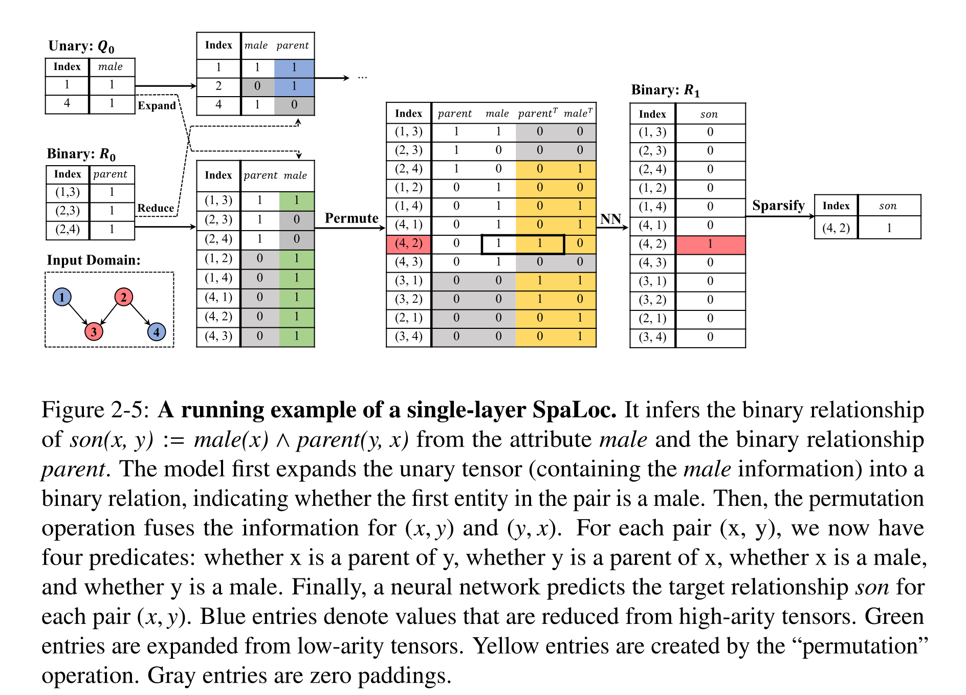
Figure 2-5: A running example of a single-layer SpaLoc. It infers the binary relationship of son(x, y) := male(x) ∧parent(y, x) from the attribute male and the binary relationship parent. The model first expands the unary tensor (containing the male information) into a binary relation, indicating whether the first entity in the pair is a male. Then, the permutation operation fuses the information for (x, y) and (y, x). For each pair (x, y), we now have four predicates: whether x is a parent of y, whether y is a parent of x, whether x is a male, and whether y is a male. Finally, a neural network predicts the target relationship son for each pair (x, y). Blue entries denote values that are reduced from high-arity tensors. Green entries are expanded from low-arity tensors. Yellow entries are created by the “permutation” operation. Gray entries are zero paddings.
Equations


Sparsification through Hoyer Regularization
The sparsification penalty sums Hoyer-Square measures of the tuple gates and normalizes by total tensor size. This ratio favors concentrating activation on fewer entries and is combined with task loss. The measure is scale-invariant, so it encourages relative concentration rather than independently forcing retained gate amplitudes to one. Appendix B compares the resulting accuracy–density tradeoff with L1 and L2 penalties.
Equations


Subgraph Training
Information sufficiency is the fraction of connecting paths retained in a sampled subgraph, approximated with a task-dependent path-length cutoff; the source defines zero divided by zero as one. Neighbor expansion selects a local induced training graph, while a target-pair path sampler can restrict inference. Positive training labels are multiplied by the sufficiency estimate; zero labels stay zero. This compensates for missing evidence heuristically. The bounded path-count statistic is not a proof that the sampled subgraph contains every fact needed by an unknown learned rule.
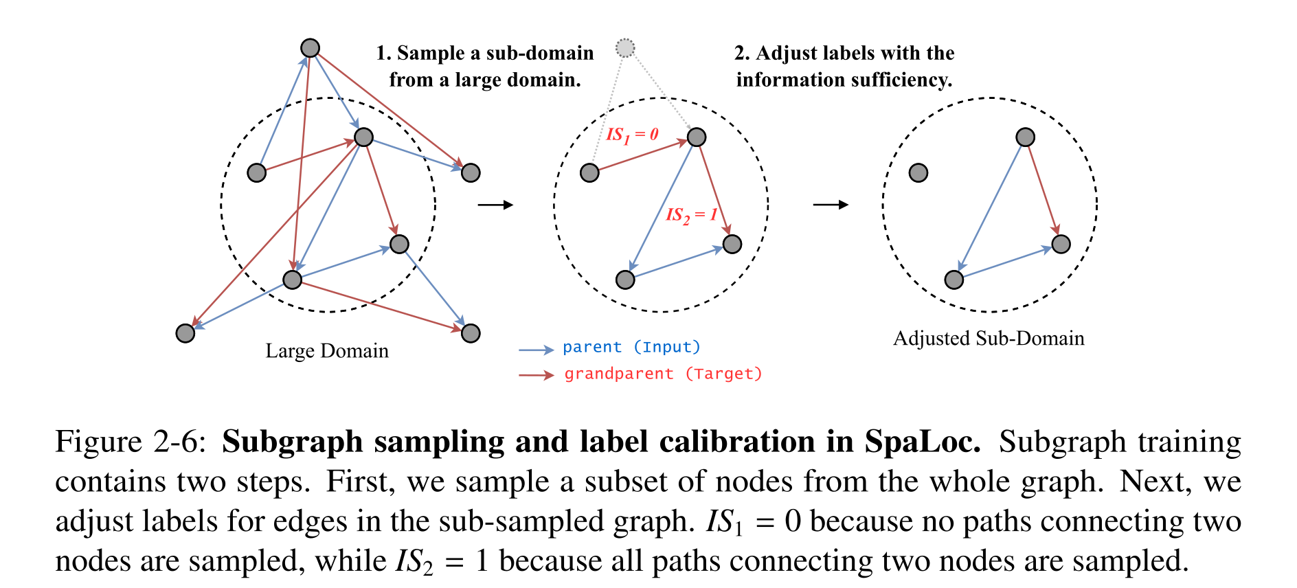
Figure 2-6: Subgraph sampling and label calibration in SpaLoc. Subgraph training contains two steps. First, we sample a subset of nodes from the whole graph. Next, we adjust labels for edges in the sub-sampled graph. IS1 = 0 because no paths connecting two nodes are sampled, while IS2 = 1 because all paths connecting two nodes are sampled.
Equations



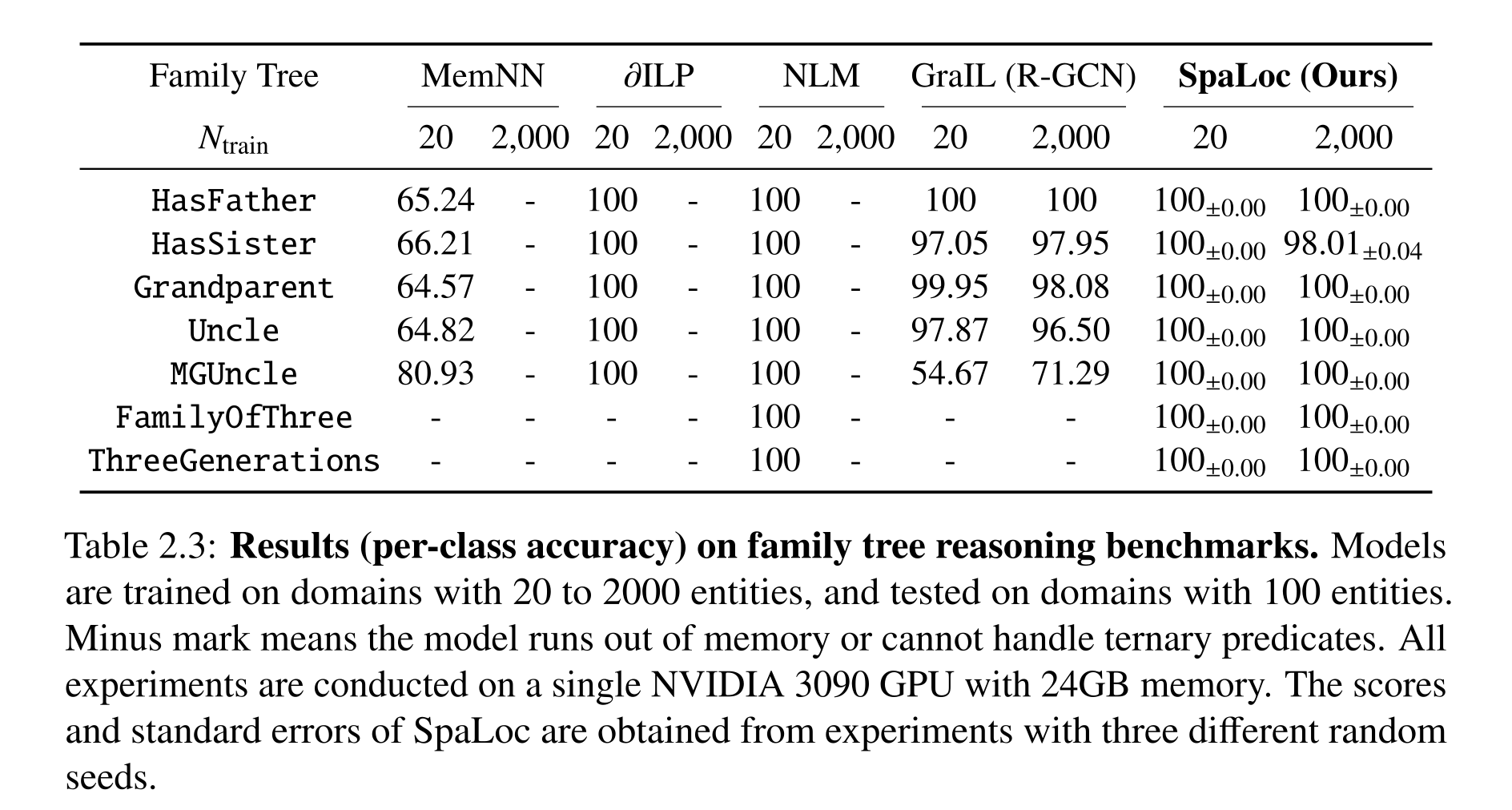
Table 2.3: Results (per-class accuracy) on family tree reasoning benchmarks. Models are trained on domains with 20 to 2000 entities, and tested on domains with 100 entities. Minus mark means the model runs out of memory or cannot handle ternary predicates. All experiments are conducted on a single NVIDIA 3090 GPU with 24GB memory. The scores and standard errors of SpaLoc are obtained from experiments with three different random seeds.
Family Tree Reasoning
SpaLoc trains on family domains up to two thousand people while tests use one hundred; it is near-perfect, with HasSister at 98.01% in the large-training setting. Three-seed errors are reported. On measured family tasks, fitted memory scaling falls from cubic toward quadratic, and both NLM and 2-GNN backbones gain speed and memory efficiency. These are empirical task-specific savings. Random-node sampling deteriorates sharply as the source graph grows, whereas walk and neighbor samplers retain useful connecting evidence and achieve 100% Grandparent accuracy.
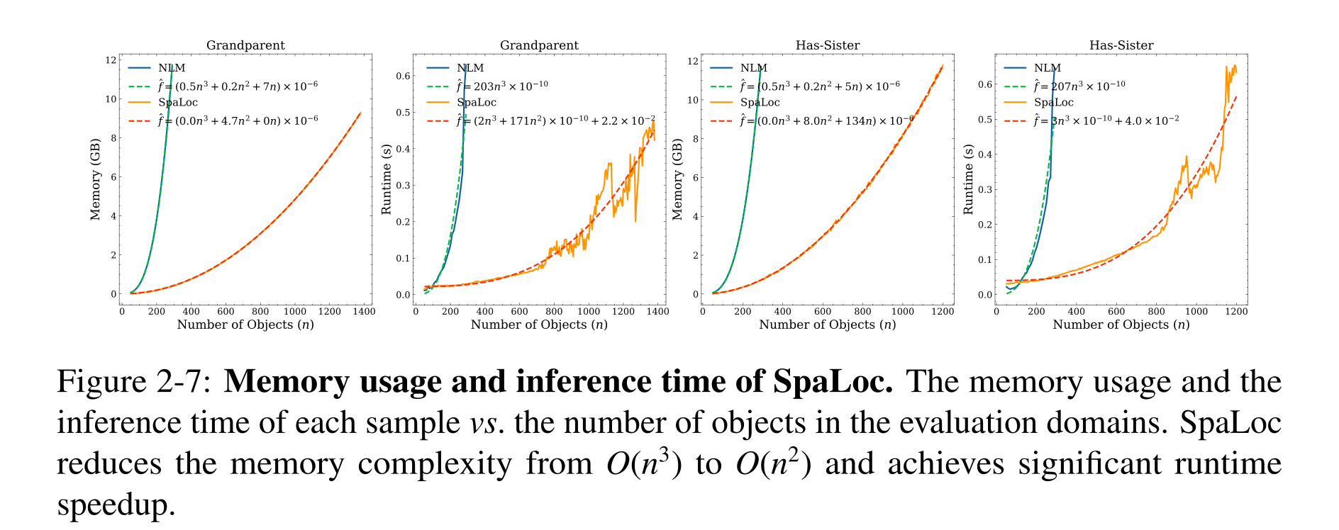
Figure 2-7: Memory usage and inference time of SpaLoc. The memory usage and the inference time of each sample vs. the number of objects in the evaluation domains. SpaLoc reduces the memory complexity from O(n3) to O(n2) and achieves significant runtime speedup.
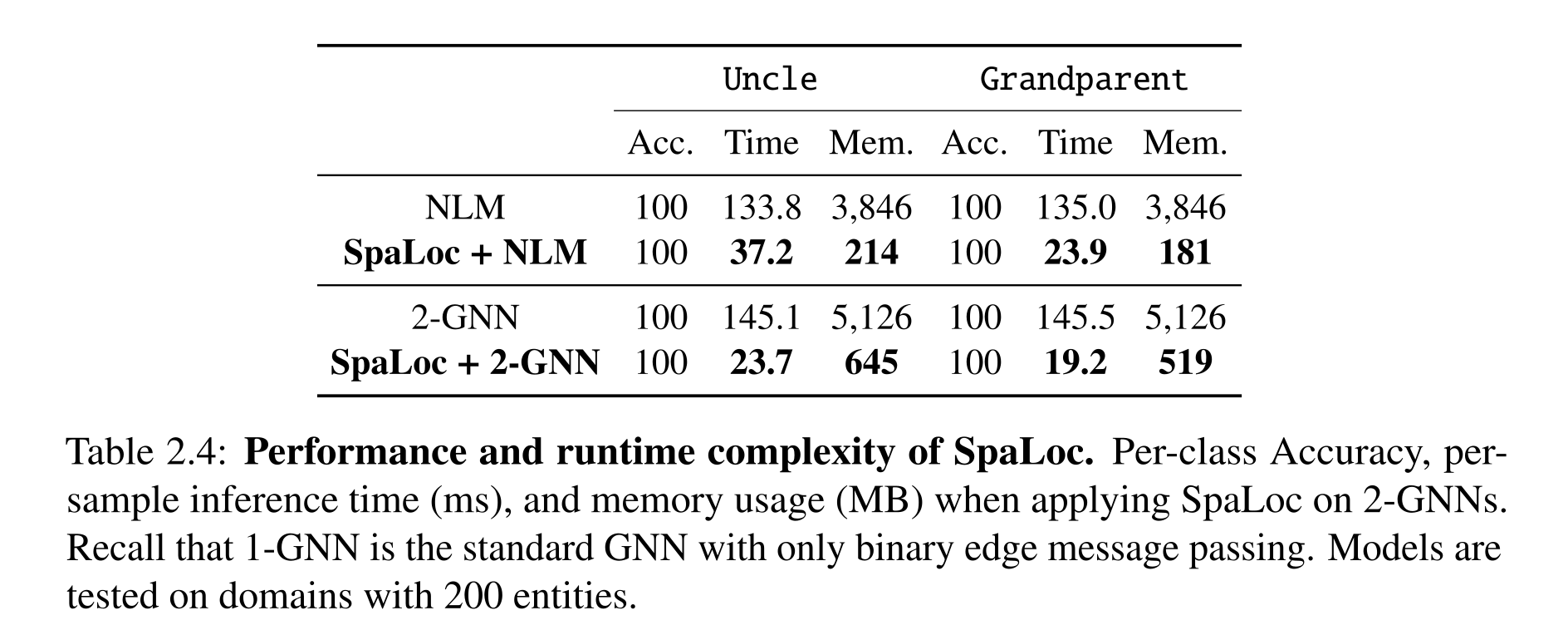
Table 2.4: Performance and runtime complexity of SpaLoc. Per-class Accuracy, per- sample inference time (ms), and memory usage (MB) when applying SpaLoc on 2-GNNs. Recall that 1-GNN is the standard GNN with only binary edge message passing. Models are tested on domains with 200 entities.
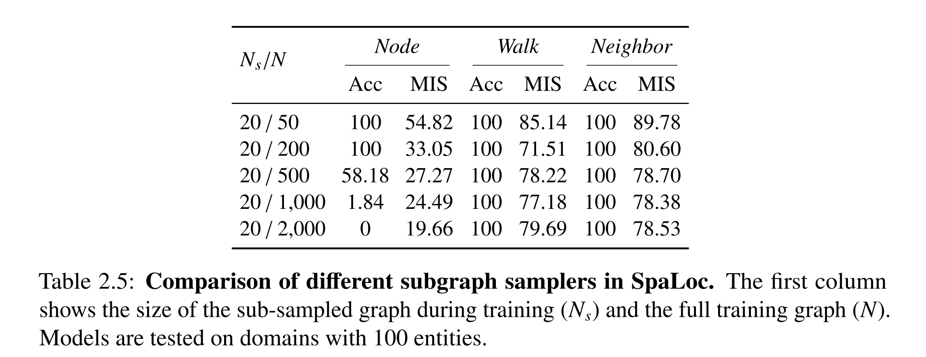
Table 2.5: Comparison of different subgraph samplers in SpaLoc. The first column shows the size of the sub-sampled graph during training (Ns) and the full training graph (N). Models are tested on domains with 100 entities.
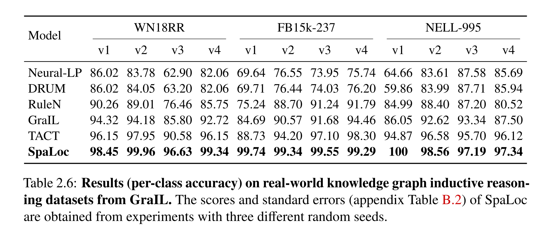
Table 2.6: Results (per-class accuracy) on real-world knowledge graph inductive reason- ing datasets from GraIL. The scores and standard errors (appendix Table B.2) of SpaLoc are obtained from experiments with three different random seeds.
Real-World Knowledge Graph Reasoning
Inductive knowledge-graph tests use disjoint training/evaluation entity subgraphs; transductive tests reuse the graph setting without storing entity-specific embeddings. The body defines AUC-PR as the classification metric despite Table 2.6’s per-class-accuracy caption. Hit@10 ranks against only fifty sampled negatives. SpaLoc improves the reported classification results, but the author explicitly reports near-zero ranking performance when negatives cover all head/tail replacements. Strong small-negative-set results therefore do not establish competitive full-entity ranking.
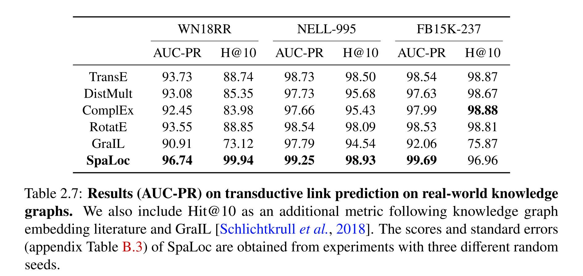
Table 2.7: Results (AUC-PR) on transductive link prediction on real-world knowledge graphs. We also include Hit@10 as an additional metric following knowledge graph embedding literature and GraIL [Schlichtkrull et al., 2018]. The scores and standard errors (appendix Table B.3) of SpaLoc are obtained from experiments with three different random seeds.
Related Work
The comparison spans ILP, differentiable proving, graph networks, relational planning, neural program induction, and efficient graph training. NLM trades explicit rule search for shared tuple computation; SpaLoc applies sparsity regularization to intermediate relation groundings and adjusts labels after subgraph sampling. These choices improve composition and scale in the demonstrated settings while leaving interpretable rule extraction, very large dense domains, and broader planning applications unresolved.
Discussion
NLM makes first-order quantification a reusable architectural structure, and SpaLoc improves its practical cost through sparse and local reasoning. The evidence supports transfer across tested object counts and empirical efficiency on selected relations. It does not remove fixed-capacity limits, difficult optimization, or failures under full knowledge-graph ranking. The following chapters extend the representation to time and analyze when relational networks can express useful planning policies.
Neuro-Symbolic Temporal Logic
Temporal and Object Quantification Networks (TOQ-Nets) extend neural logic machines from static relations to event classification. Shared object and time pooling supports variable entity counts and sequence durations; experiments test soccer events, robot manipulation trajectories, and human activities. The chapter builds on Mao et al. (2021).
Introduction
A pass or an opening action depends on relations that change in a particular order. TOQ-Nets learn soft predicates and compositions from sequence labels, using finite-domain object quantification and a restricted form of linear temporal logic. This supplies a structural bias for transferring learned event concepts across object counts and timings without requiring a manually written rule for each action.
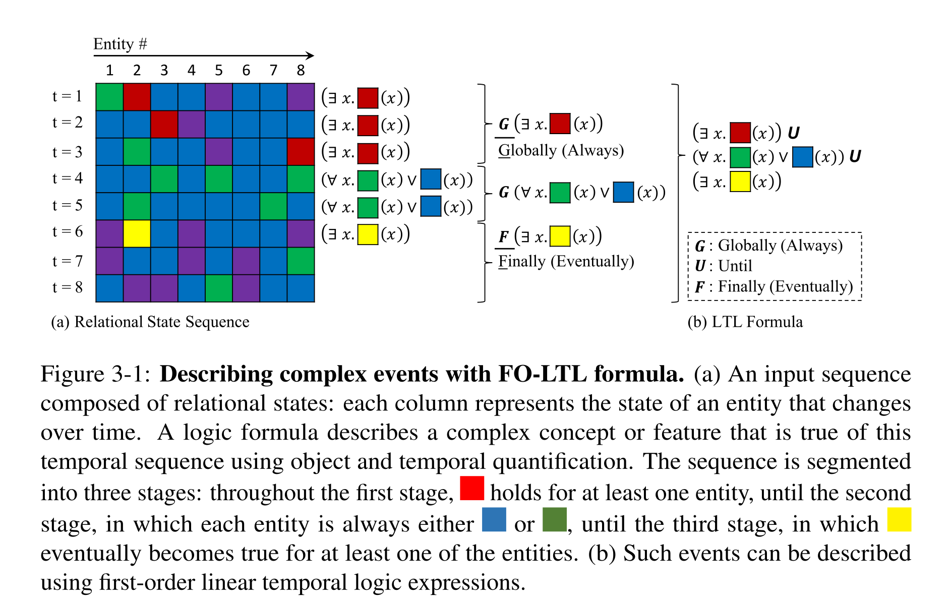
Figure 3-1: Describing complex events with FO-LTL formula. (a) An input sequence composed of relational states: each column represents the state of an entity that changes over time. A logic formula describes a complex concept or feature that is true of this temporal sequence using object and temporal quantification. The sequence is segmented into three stages: throughout the first stage, holds for at least one entity, until the second stage, in which each entity is always either or , until the third stage, in which eventually becomes true for at least one of the entities. (b) Such events can be described using first-order linear temporal logic expressions.
TOQ-Nets
The pipeline extracts local physical features, applies relational reasoning independently at each time, reduces entities to global event features, and applies temporal reasoning before classifying the sequence from its initial-time summary. Parameters are shared across entities and times. Fixed depth bounds logical nesting, quantifiers range only over the observed finite sequence, and the implemented architecture covers a subset of first-order temporal logic.
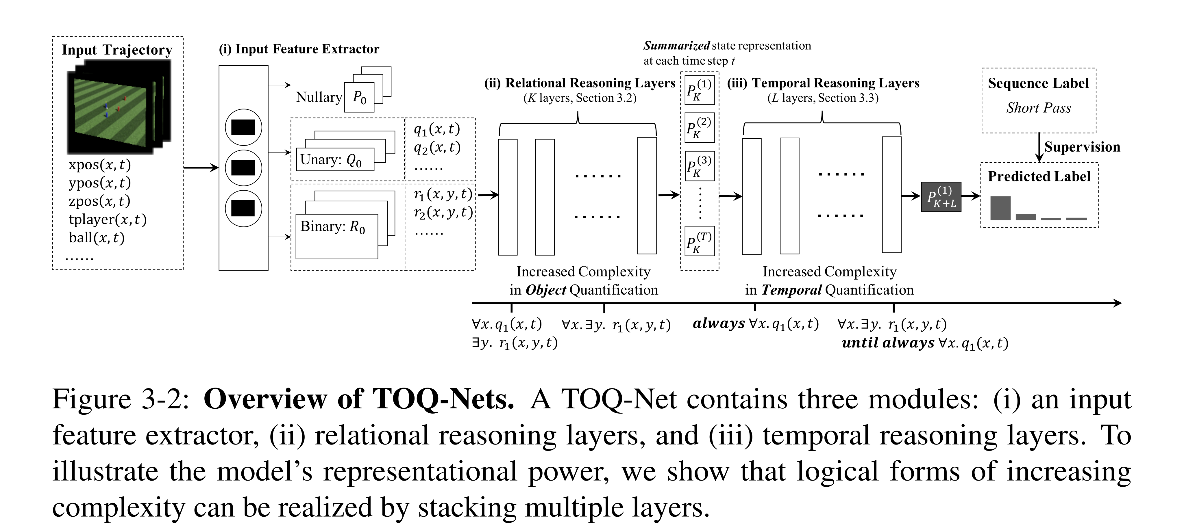
Figure 3-2: Overview of TOQ-Nets. A TOQ-Net contains three modules: (i) an input feature extractor, (ii) relational reasoning layers, and (iii) temporal reasoning layers. To illustrate the model’s representational power, we show that logical forms of increasing complexity can be realized by stacking multiple layers.
Temporal-Relational Feature Representation
At each time, nullary features form a vector, unary features an entity-by-channel matrix, and binary relations an entity-by-entity-by-channel tensor. Adding the time axis represents all grounded relations in parallel. Soccer inputs include entity coordinates and type/team indicators; relational tensors subsequently express learned interactions rather than one fixed vector per scene.
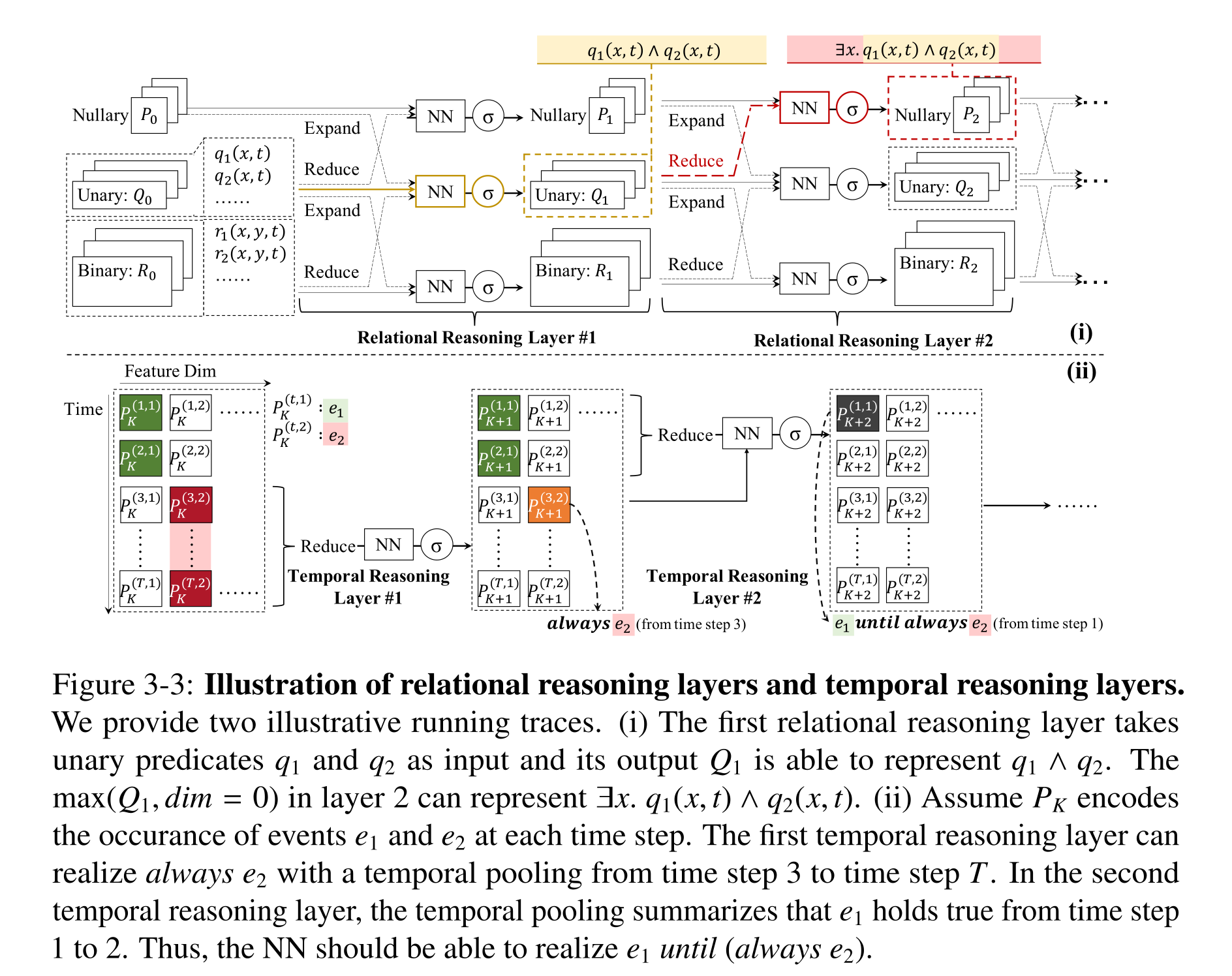
Figure 3-3: Illustration of relational reasoning layers and temporal reasoning layers. We provide two illustrative running traces. (i) The first relational reasoning layer takes unary predicates q1 and q2 as input and its output Q1 is able to represent q1 ∧q2. The max(Q1, dim = 0) in layer 2 can represent ∃x. q1(x, t) ∧q2(x, t). (ii) Assume PK encodes the occurance of events e1 and e2 at each time step. The first temporal reasoning layer can realize always e2 with a temporal pooling from time step 3 to time step T. In the second temporal reasoning layer, the temporal pooling summarizes that e1 holds true from time step 1 to 2. Thus, the NN should be able to realize e1 until (always e2).
Relational Reasoning Layers
Each relational layer concatenates features at adjacent arities using broadcasting and max reductions, then applies shared affine maps with sigmoid activations. Max pooling realizes soft existential quantification; learned negation can express universal quantification through its dual. Pooling both arguments of binary tensors preserves directional roles. The same layer runs at every time; this chapter uses arity at most two, although the construction extends to higher arities.
Equation

Temporal Reasoning Layers
Temporal layers pool event features over intervals and combine them with a candidate future endpoint, then pool over endpoints. The first layer instead summarizes suffixes; residual connections retain the unpooled features. Stacking layers can express sequences of eventually/until conditions such as an event holding until another becomes persistent, with quadratic space in sequence length. The actual endpoint enumeration is strict, t′ > t, as shown by the running algorithm. With all relational layers preceding temporal layers, object quantification is nested inside temporal quantification: “always some object has a property” is expressible, but “one object always has it” requires interleaving the layer types.
Equations


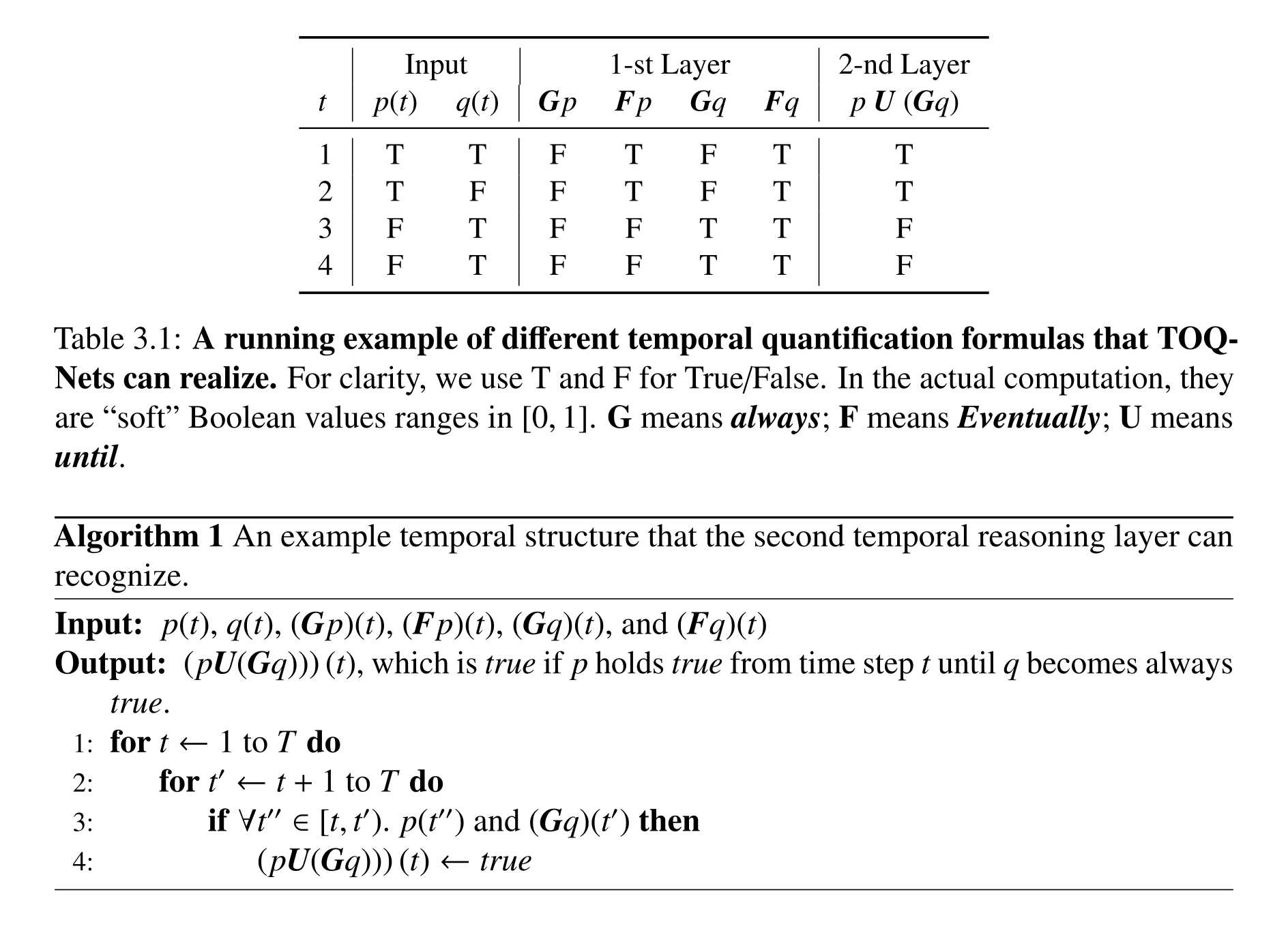
Table 3.1: A running example of different temporal quantification formulas that TOQ- Nets can realize. For clarity, we use T and F for True/False. In the actual computation, they are “soft” Boolean values ranges in [0, 1]. G means always; F means Eventually; U means until.
Equations


Experiments
Evaluation separates ordinary classification from few-shot transfer, changes in entity count, and temporal distortions. Inputs are tracked physical states or annotated features, so these experiments principally test relational and temporal reasoning rather than complete visual perception.
Baseline Approaches
Comparisons include spatiotemporal graph convolution (STGCN), max-pooling and LSTM variants, space-time region graphs, and non-local attention. Capacity and input-feature ablations in Appendix C help distinguish temporal reasoning from parameter count and access to pairwise distances.
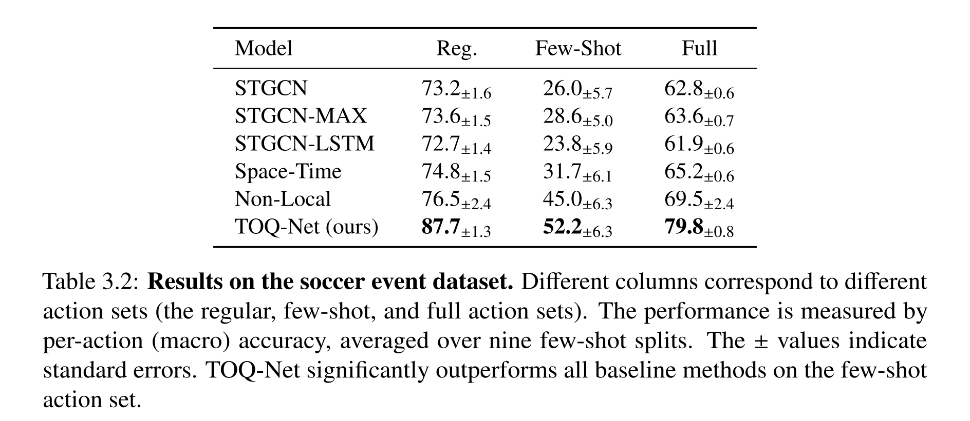
Table 3.2: Results on the soccer event dataset. Different columns correspond to different action sets (the regular, few-shot, and full action sets). The performance is measured by per-action (macro) accuracy, averaged over nine few-shot splits. The ± values indicate standard errors. TOQ-Net significantly outperforms all baseline methods on the few-shot action set.
Trajectory-Based Soccer Event Detection
Simulator soccer data contains nine action categories; seven receive the full training set and two only 50 clips each. TOQ-Net reaches 79.8% macro accuracy overall and 52.2% on few-shot classes, versus 69.5% and 45.0% for the strongest listed non-local baseline. Training on 6v6 games gives 88.4% ordinary accuracy, 77.1% on 11v11, and 86.9% on time-warped 6v6 sequences. Larger games still cause errors: shot recall falls from 97% to 60% when failed shots resemble passes. Small-data finetuning helps transfer to changed spatial/temporal scales; depth and capacity ablations favor three relational and four temporal layers in the main text. Gradient-based feature visualizations illustrate learned dependencies without establishing an exact symbolic program. The dataset description mentions both 25-frame contexts and 17-frame clips, while the temporal-shift test explicitly uses 25 frames.
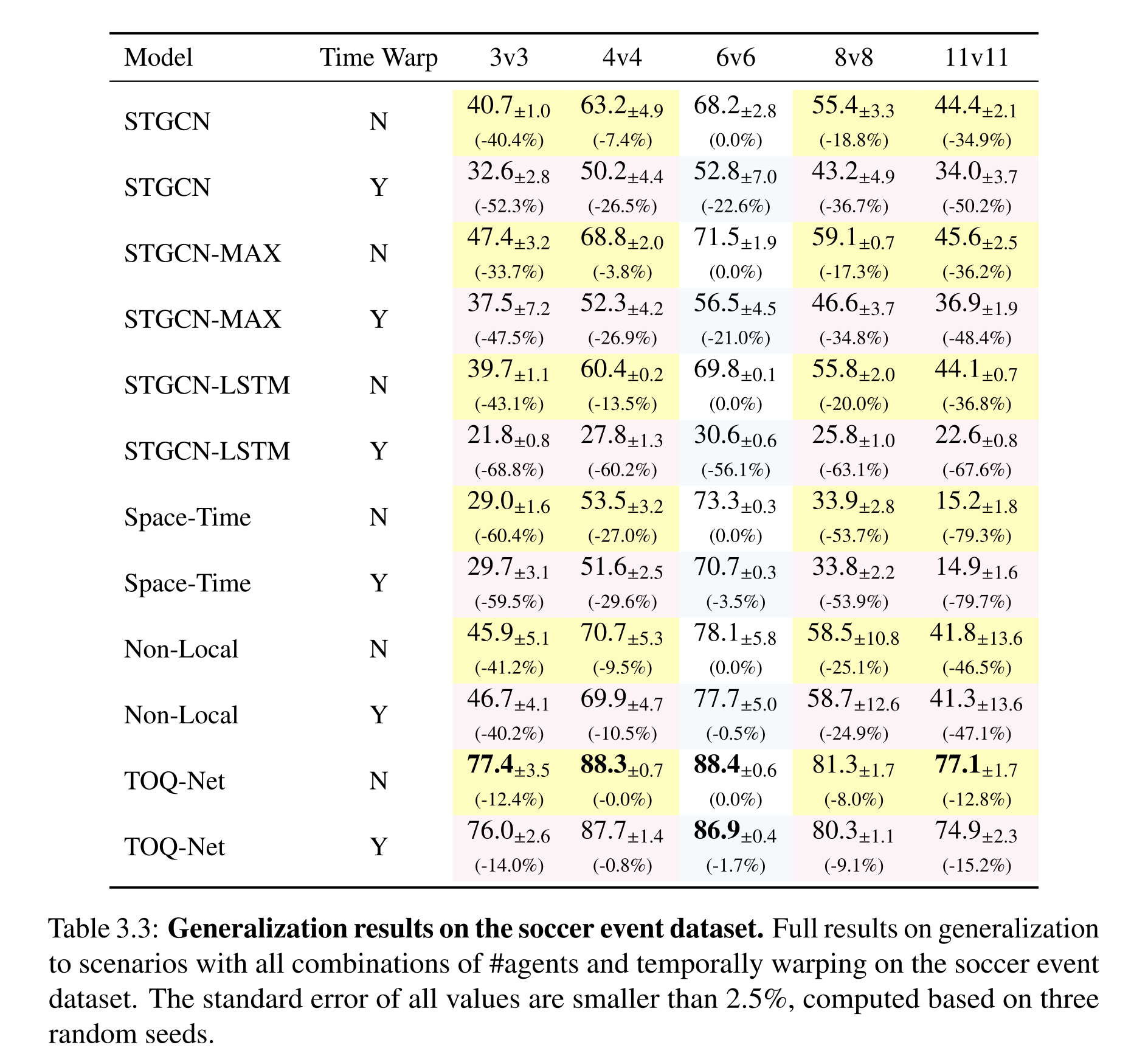
Table 3.3: Generalization results on the soccer event dataset. Full results on generalization to scenarios with all combinations of #agents and temporally warping on the soccer event dataset. The standard error of all values are smaller than 2.5%, computed based on three random seeds.
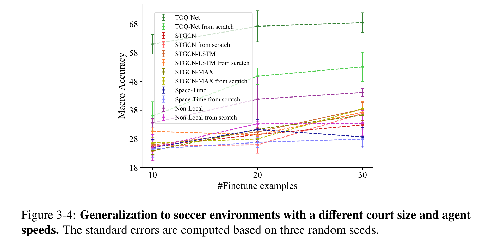
Figure 3-4: Generalization to soccer environments with a different court size and agent speeds. The standard errors are computed based on three random seeds.
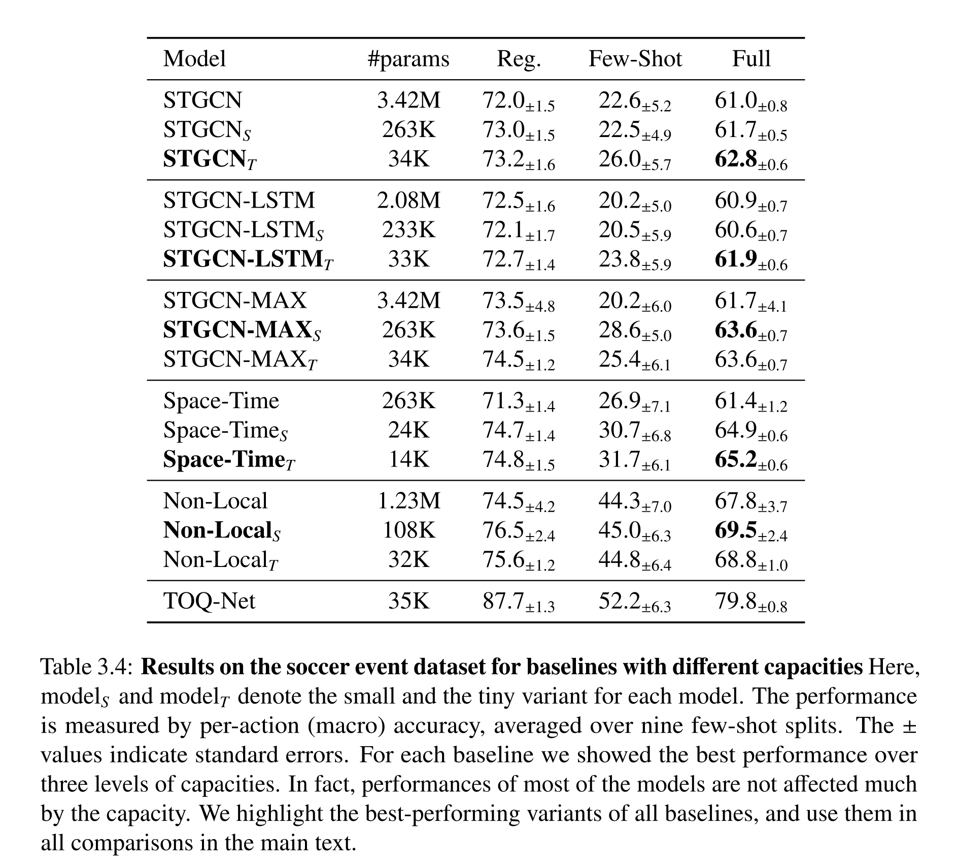
Table 3.4: Results on the soccer event dataset for baselines with different capacities Here, modelS and modelT denote the small and the tiny variant for each model. The performance is measured by per-action (macro) accuracy, averaged over nine few-shot splits. The ± values indicate standard errors. For each baseline we showed the best performance over three levels of capacities. In fact, performances of most of the models are not affected much by the capacity. We highlight the best-performing variants of all baselines, and use them in all comparisons in the main text.
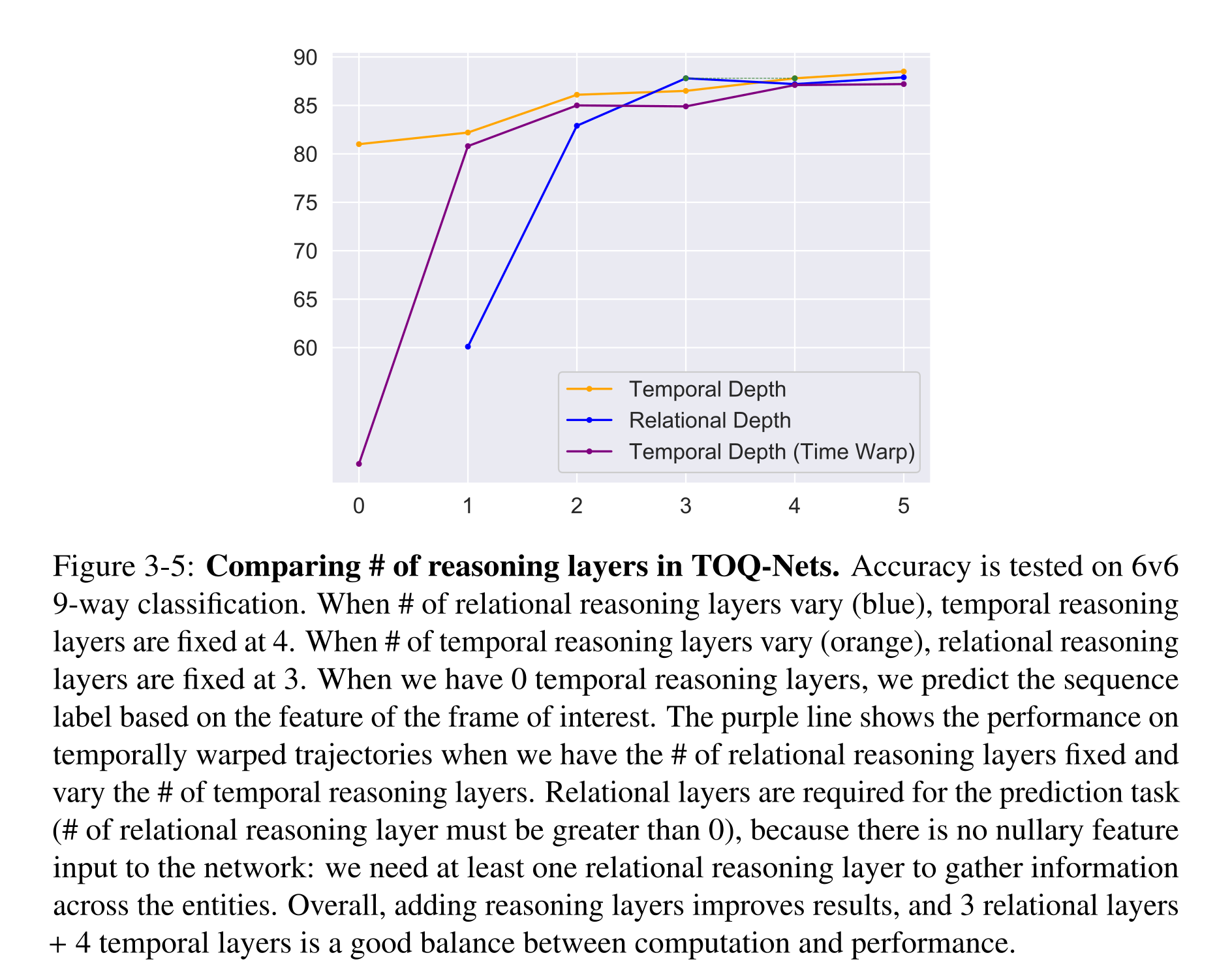
Figure 3-5: Comparing # of reasoning layers in TOQ-Nets. Accuracy is tested on 6v6 9-way classification. When # of relational reasoning layers vary (blue), temporal reasoning layers are fixed at 4. When # of temporal reasoning layers vary (orange), relational reasoning layers are fixed at 3. When we have 0 temporal reasoning layers, we predict the sequence label based on the feature of the frame of interest. The purple line shows the performance on temporally warped trajectories when we have the # of relational reasoning layers fixed and vary the # of temporal reasoning layers. Relational layers are required for the prediction task (# of relational reasoning layer must be greater than 0), because there is no nullary feature input to the network: we need at least one relational reasoning layer to gather information across the entities. Overall, adding reasoning layers improves results, and 3 relational layers + 4 temporal layers is a good balance between computation and performance.
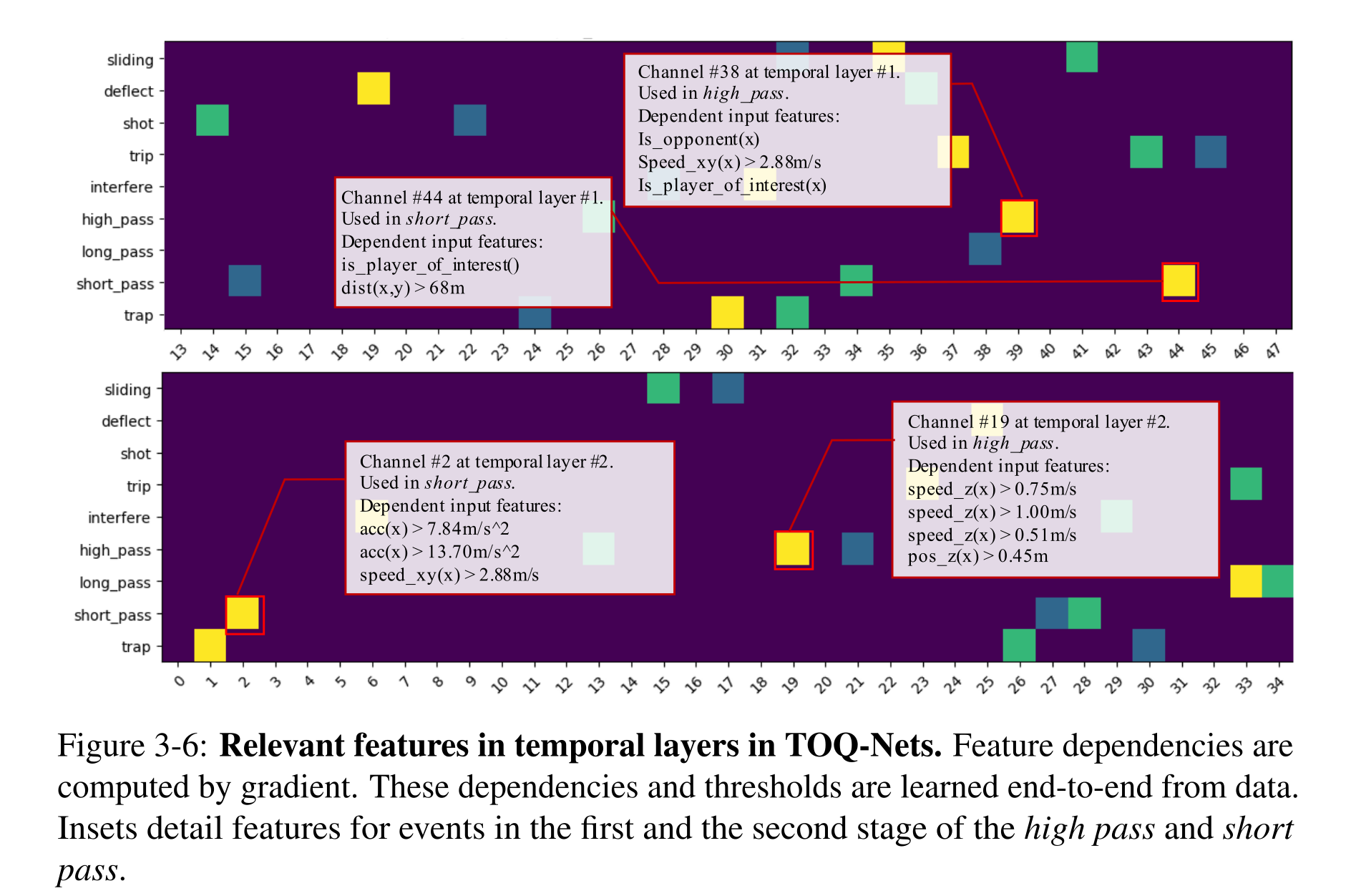
Figure 3-6: Relevant features in temporal layers in TOQ-Nets. Feature dependencies are computed by gradient. These dependencies and thresholds are learned end-to-end from data. Insets detail features for events in the first and the second stage of the high pass and short pass.
Manipulation Concept Learning from 6D Poses
RLBench supplies 100 motion-planned trajectories for each of 24 actions, with varying lengths and object/gripper poses as inputs. Standard classification and time stretching from one eighth to eight times the original duration favor TOQ-Net. A separate three-way Open-X/Close-X/Other test with held-out object actions seen once yields 98.04% macro accuracy on the one-shot subset and 99.48% overall. Closing jars and drawers remains harder because rotation and pushing differ from other closing motions. These are action-recognition results on simulated trajectories, not learned execution policies.
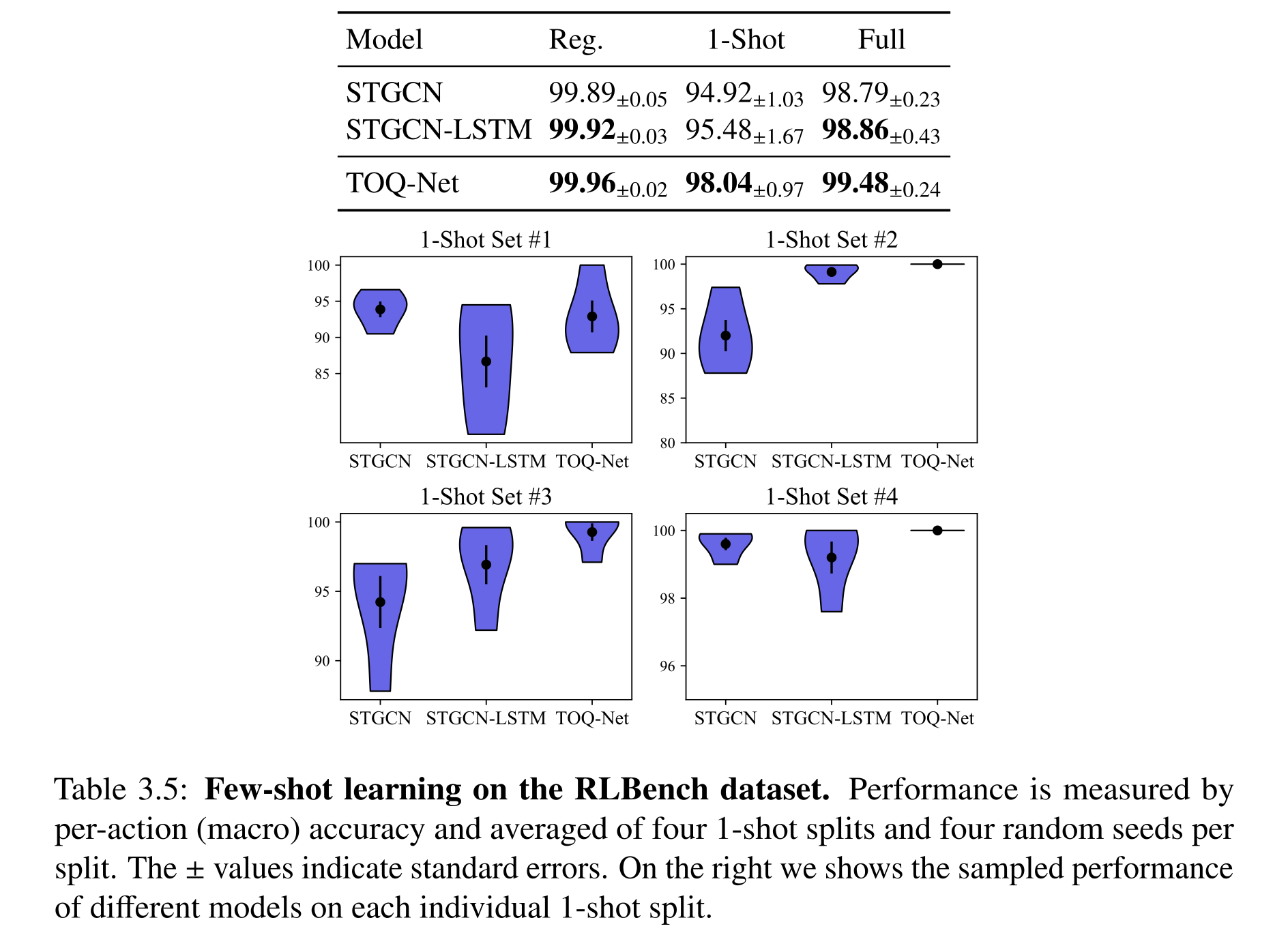
Table 3.5: Few-shot learning on the RLBench dataset. Performance is measured by per-action (macro) accuracy and averaged of four 1-shot splits and four random seeds per split. The ± values indicate standard errors. On the right we shows the sampled performance of different models on each individual 1-shot split.
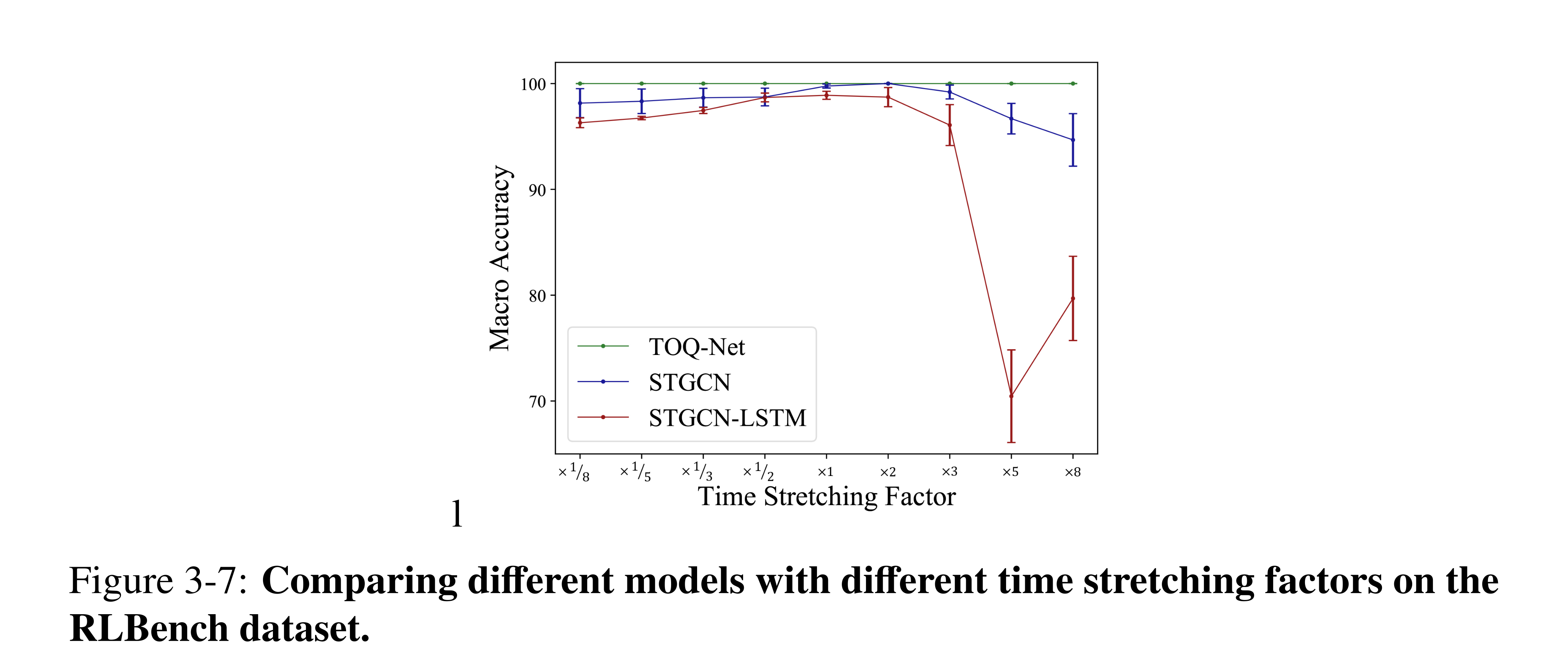
Figure 3-7: Comparing different models with different time stretching factors on the RLBench dataset.
Extension to Real-World Datasets
On Toyota Smarthome skeletons, TOQ-Net is comparable to STGCN on ordinary classification (42.0% versus 43.0%) but retains 41.2% under doubled speed, where STGCN falls to 32.3%. On volleyball, manually annotated player features give 73.3% versus 73.6% ordinarily; TOQ-Net retains about 70% under time shifts and faster motion while STGCN falls to 39.5% and 48.6%. The gain is robustness to temporal variation, not higher standard accuracy on every dataset.
Related Work
Symbolic event systems and temporal-logic synthesis offer explicit descriptions but often require annotated primitives or combinatorial rule search. Neural graph and recurrent approaches learn representations from data. TOQ-Nets combine end-to-end feature learning with explicit finite object/time quantification, using a different temporal inductive bias from convolution, recurrence, or order-agnostic aggregation.
Discussion
Object/time pooling improves transfer across observed entity counts and time courses, but fixed depth and the chosen ordering of quantifiers limit expressiveness. Generalization to substantially different object kinds remains open, and physical trajectories alone can confuse unsuccessful intentions with successful actions of another class. Modeling goals, beliefs, and intentions is proposed as a next step; the temporal structures also motivate later action-precondition/postcondition models.
Expressiveness of Neuro-Symbolic Logic Models
This chapter connects classical planning search to relational policy circuits. Serialized goal regression provides constructive upper bounds on network breadth and depth, explaining why some object-centric tasks admit policies that scale across instance sizes while others require growing computation. The analysis builds on Mao et al. (2023) and Luo et al. (2021); empirical learning experiments test selected implications rather than proving learnability in general.
Introduction
A goal-conditioned network produces the next action from a state and goal, but compact parameters do not guarantee that it can represent a successful planner. The chapter relates regression width and planning horizon to the size of a parameter-sharing relational circuit. It constructs policies for restricted classical domains and studies when resource conflicts prevent simple subgoal decomposition; unrestricted STRIPS planning remains computationally hard.
Preliminaries: Planning Domain and Problem
States are finite sets of true ground atoms over a fixed object universe; omitted atoms are false. STRIPS action schemas specify positive preconditions and add/delete effects, yielding deterministic partial transitions. Planning finds an action sequence, whereas a goal-conditioned policy is applied repeatedly to produce one. The analysis uses a single goal atom; conjunctive goals can be encoded with an extra achievement action, but this transformation does not preserve all small-width or optimal-serialization advantages.
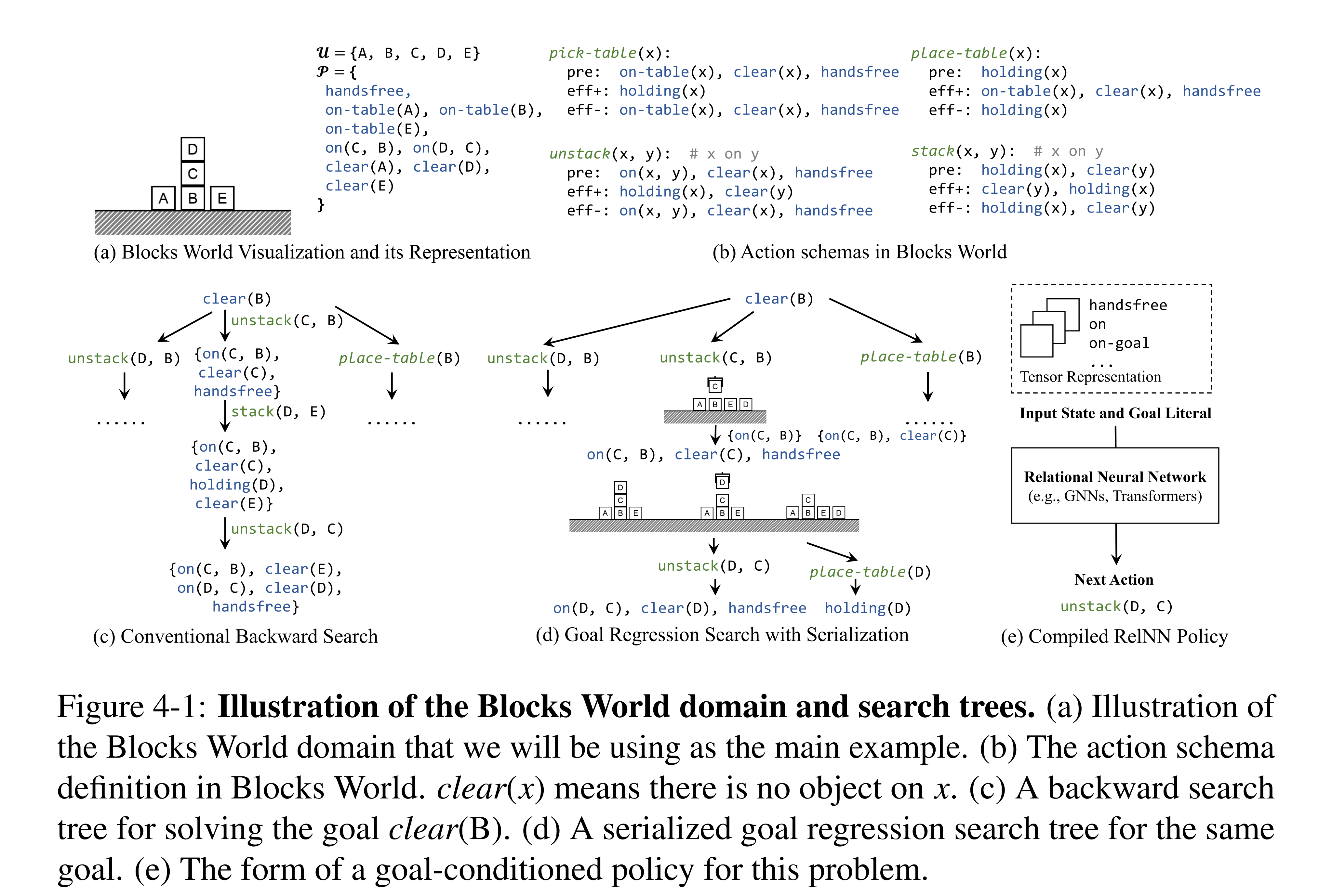
Figure 4-1: Illustration of the Blocks World domain and search trees. (a) Illustration of the Blocks World domain that we will be using as the main example. (b) The action schema definition in Blocks World. clear(x) means there is no object on x. (c) A backward search tree for solving the goal clear(B). (d) A serialized goal regression search tree for the same goal. (e) The form of a goal-conditioned policy for this problem.
Goal Regression Search and Width
Plain backward search repeatedly replaces desired effects with action preconditions, keeping conjunctive goal sets and rejecting cycles. Both growing goal sets and long horizons can make this search expensive. Serialized goal regression instead tries an ordering of preconditions and explicitly tracks facts that must remain true, making the source of combinatorial width more visible.
Serialized Goal Regression Search
A regression rule achieves one goal by solving an ordered precondition list and then executing its final action. Each subproblem preserves the external constraints and previously achieved preconditions. All candidate rules can be obtained by permuting action preconditions. The simplified algorithm keeps a shortest result at each step, but is neither complete nor optimal for arbitrary domains: different ways of reaching one subgoal can affect whether later ones remain achievable.
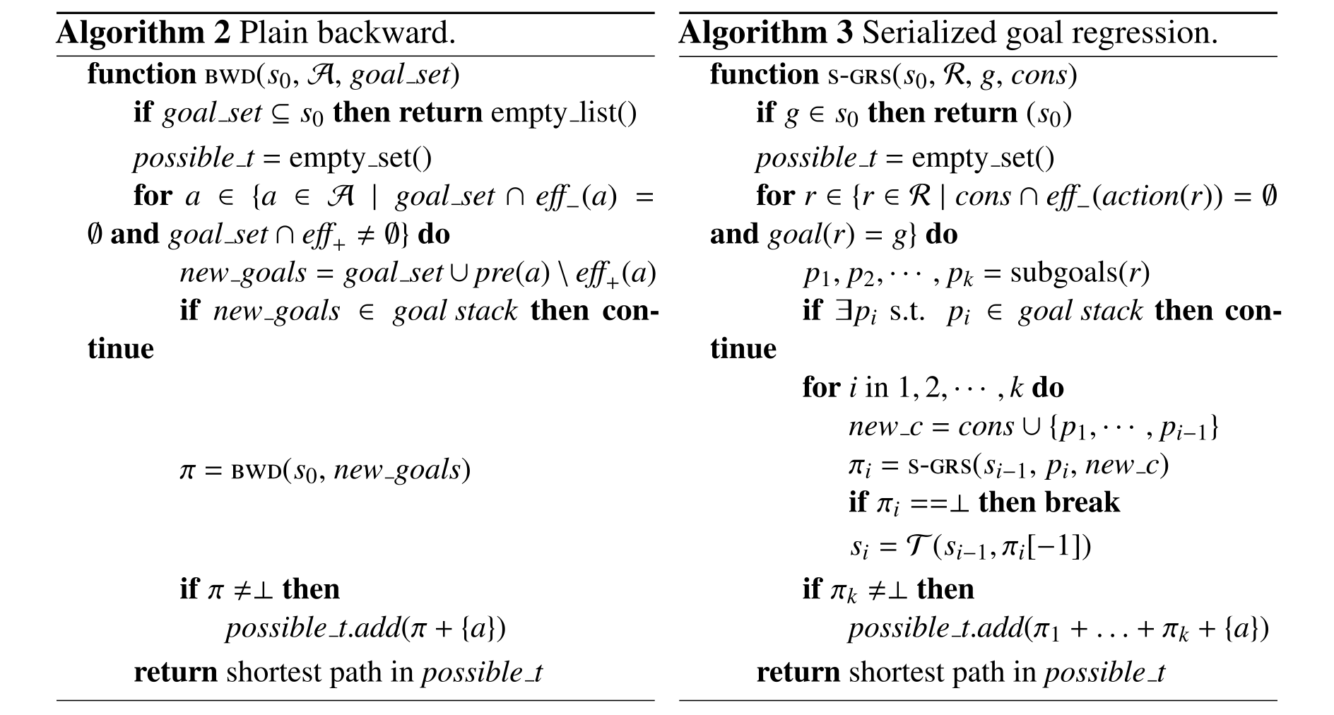
Complete original algorithm group.
Serialization of Goal Regression Rules
Optimal serializability requires every optimal solution of a precondition prefix to extend, through an optimal next-subgoal solution, to an optimal solution of the longer prefix; satisfying all preconditions followed by the final action must also be optimal for the goal. Under the stated set of solvable optimally serializable goals, S-GRS is complete and optimal. These are domain/state conditions, not properties of arbitrary subgoal orderings.
Width of Search Problems
Generalized rules retain only the prior facts that need explicit protection. Width counts these retained constraints; strong optimal serializability (SOS) additionally ensures that solving the reduced subproblem preserves the full prefix under added constraints. For SOS width k, the stated search bound is O(Nk+1) in the number of atoms, suppressing polynomial action/serialization factors. SOS is essential to reuse reduced subproblems. SOS width k implies forward width at most k+1 and solvability by IW(k+1), but the two width notions are not equal.
Policy Realization
Relational policies accept state and goal tensors of variable object count with shared parameters. Breadth measures maximum tuple arity; depth measures sequential computation. The chapter first compiles general and serialized search into such circuits, then shows how a suitable rule selector can reduce the work further. Constant breadth still permits depth and grounded circuit size to grow with the instance.
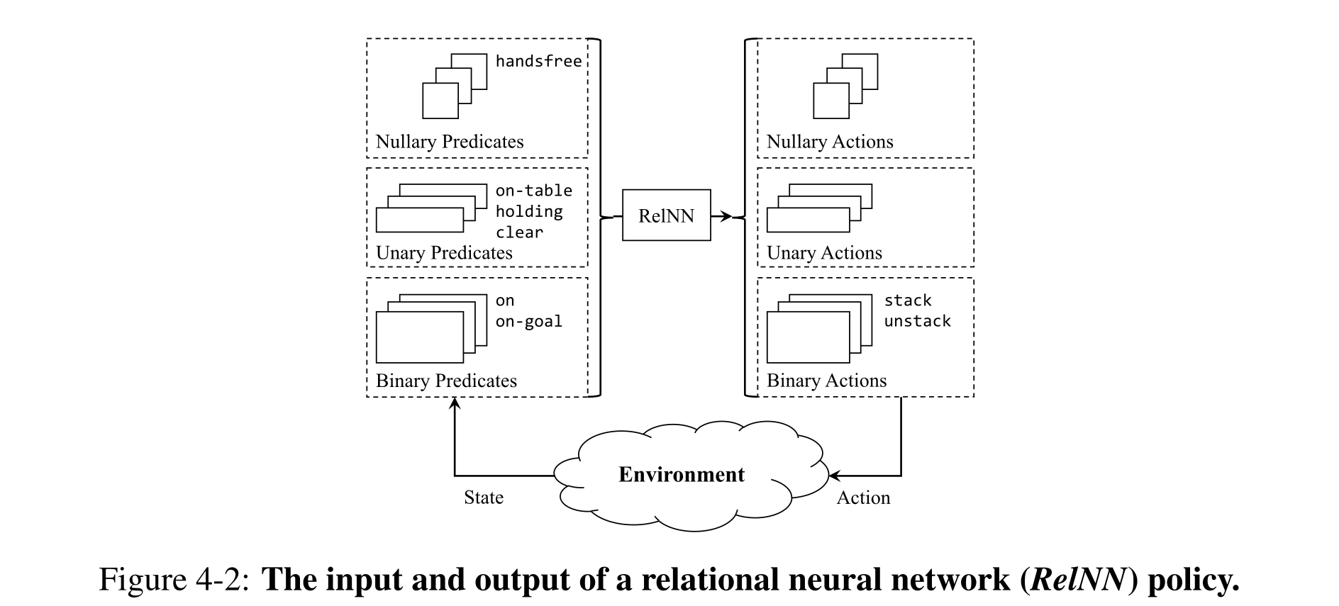
Figure 4-2: The input and output of a relational neural network (RelNN) policy.
Relational Neural Network Expressiveness
Increasing intermediate arity strictly increases relational-network expressiveness under the stated Weisfeiler–Leman connection. B-variable first-order logic with counting motivates breadth-B constructions, with sum aggregation providing counting; this extends beyond a max-only NLM layer. Hidden-channel capacity is assumed sufficient. The proposed fixed-precision depth hierarchy is explicitly a conjecture, not a theorem; its separation is not transferred to unbounded-precision networks, which the source says saturate at a bounded polynomial depth.
Compilation of BWD and S-GRS
Backward search with maximum conjunctive goal size kBWD compiles to depth O(T) and breadth βkBWD, where T is optimal plan length and β maximum predicate arity. SOS width k yields the stated breadth bound β(k+1) at the same O(T) depth. Serialization can therefore bound breadth even when ordinary regression goal sets grow, but neither construction guarantees a shallow policy when the required horizon grows.
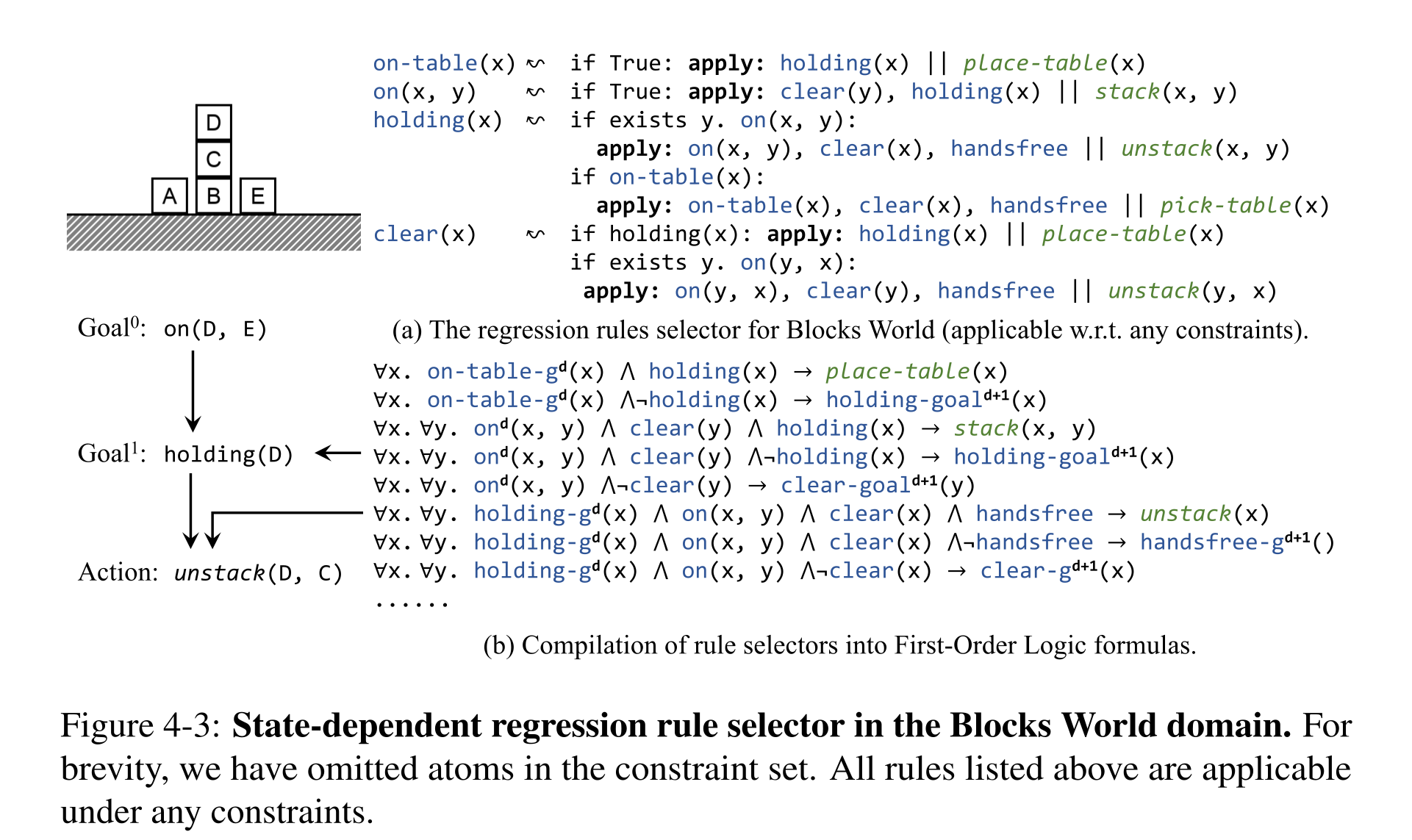
Figure 4-3: State-dependent regression rule selector in the Blocks World domain. For brevity, we have omitted atoms in the constraint set. All rules listed above are applicable under any constraints.
Compilation of S-GRS with a Regression Rule Selector
A state-dependent regression-rule selector chooses an operator, precondition order, and bindings without exhaustive branching. If it is serializable and computable with depth Dr and breadth Br, the resulting next-action circuit has stated depth O(dDr) and breadth max(Br,β), where d is regression-tree depth. The policy follows the first unsatisfied subgoal in the current state. The selector may be supplied or learned; its existence and correctness are additional assumptions. A logarithmic relation between tree depth and plan length requires branching structure and is not a general guarantee for chain-like regressions. Recurrent layers or explicitly supplied shortcut predicates can handle some growing-depth cases.
Equation

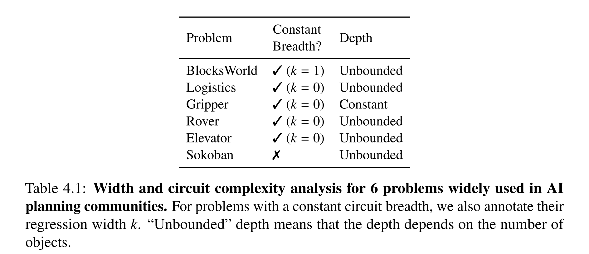
Table 4.1: Width and circuit complexity analysis for 6 problems widely used in AI planning communities. For problems with a constant circuit breadth, we also annotate their regression width k. “Unbounded” depth means that the depth depends on the number of objects.
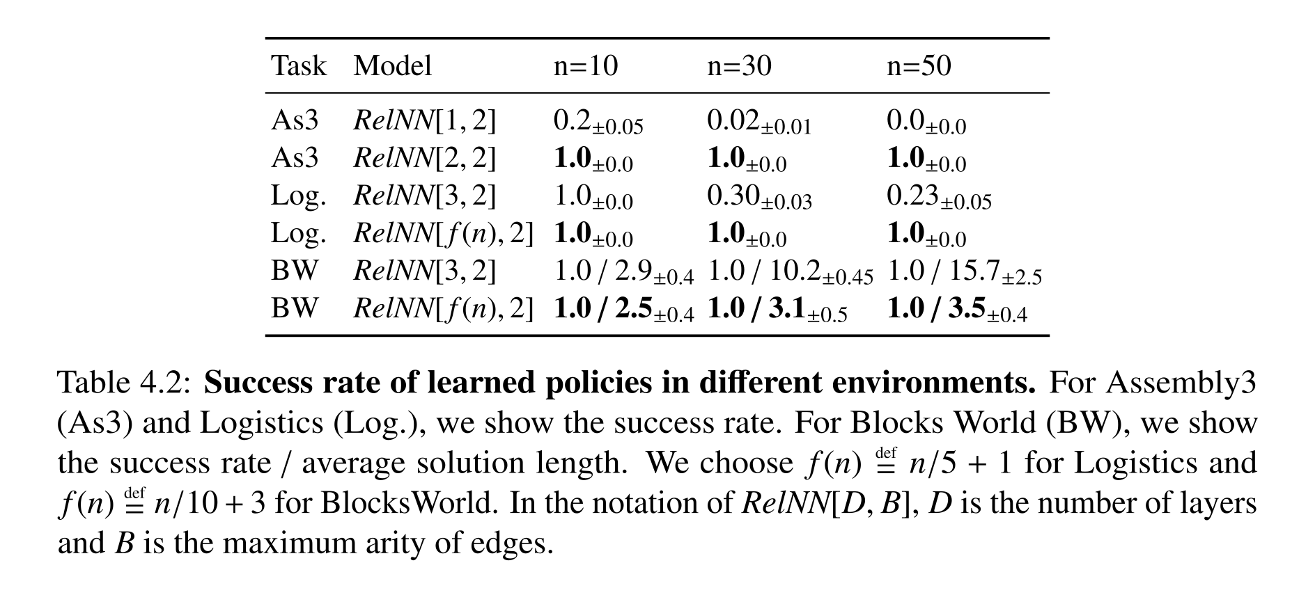
Table 4.2: Success rate of learned policies in different environments. For Assembly3 (As3) and Logistics (Log.), we show the success rate. For Blocks World (BW), we show the success rate / average solution length. We choose f(n) def= n/5 + 1 for Logistics and f(n) def= n/10 + 3 for BlocksWorld. In the notation of RelNN[D, B], D is the number of layers and B is the maximum arity of edges.
Problem Analysis and Results
For single-atom goals, the analysis assigns constant breadth to BlocksWorld, Logistics, Gripper, Rover, and Elevator, while Sokoban lacks the proposed bounded-width serialization. Most listed domains still need instance-dependent depth; Gripper assumes direct travel between rooms. Three-seed experiments support selected depth predictions: a two-layer Assembly3 policy generalizes from 10 to 50 objects where one layer fails; adaptive-depth Logistics reaches 100% at 50 cities versus 23% for three layers. Both BlocksWorld policies succeed, but adaptive depth reduces average plan length at 50 objects from 15.7 to 3.5. These results concern constructed task distributions and chosen depth schedules, not universal learned planning guarantees.
Related Work
The analysis combines classical planning complexity and width, hierarchical/subgoal serialization, and logical characterizations of relational neural networks. Its distinctive link is constructive compilation of search into a next-action policy. This complements empirical algorithmic-alignment and graph-size generalization studies rather than replacing their learning assumptions.
Discussion
Regression width characterizes how many facts must be protected while decomposing a goal, while policy depth reflects the amount of sequential reasoning. Resource constraints can obstruct small circuits, and the constructive upper bounds do not establish easy optimization or learning. The proofs concern discrete fully specified domains; extending them to continuous actions, uncertain transitions, or policies shared across many domains remains open.
Neuro-Symbolic Continuous Constraint Satisfaction
Diffusion-CCSP learns modular continuous constraint models and composes them to generate assignments for new factor graphs. It targets geometric, physical, and qualitative constraints in robot planning, complementing the preceding chapters’ logical deduction. The chapter builds on Yang et al. (2023); experiments demonstrate useful compositional sampling rather than a complete or certified constraint solver.
Introduction
A feasible placement must jointly respect geometry, stability, grasps, motion, and task requirements. Sequential samplers can waste effort when later constraints invalidate earlier choices, while hand-written differentiable objectives are difficult for qualitative relations. Diffusion-CCSP associates a learned model with each constraint type and combines their updates over a graph, allowing new combinations and larger instances built from known types.
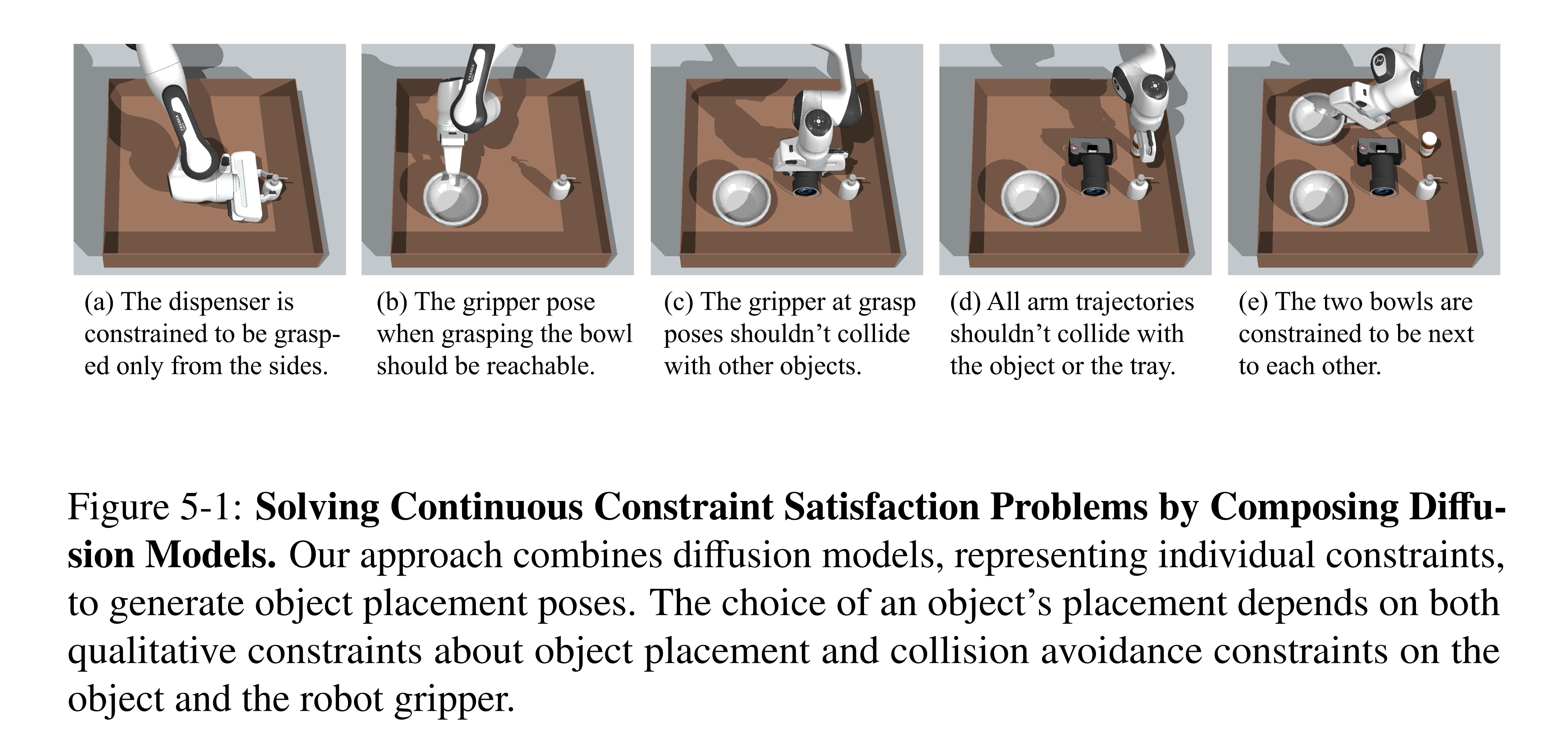
Figure 5-1: Solving Continuous Constraint Satisfaction Problems by Composing Diffu- sion Models. Our approach combines diffusion models, representing individual constraints, to generate object placement poses. The choice of an object’s placement depends on both qualitative constraints about object placement and collision avoidance constraints on the object and the robot gripper.
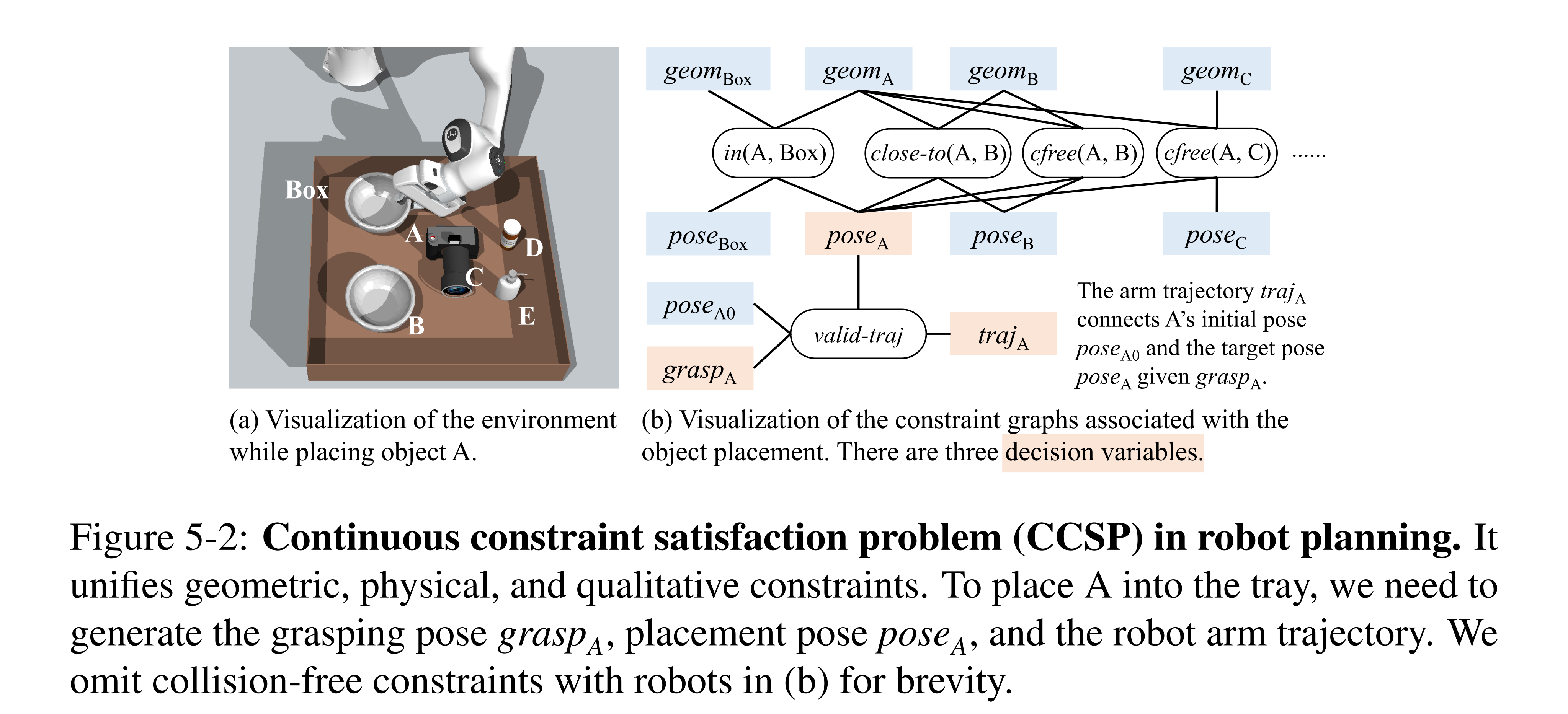
Figure 5-2: Continuous constraint satisfaction problem (CCSP) in robot planning. It unifies geometric, physical, and qualitative constraints. To place A into the tray, we need to generate the grasping pose graspA, placement pose poseA, and the robot arm trajectory. We omit collision-free constraints with robots in (b) for brevity.
Compositional Diffusion Constraint Solvers
A factor graph separates decision variables from fixed conditioning information and records each constraint’s scope. Learned denoisers share parameters across occurrences of the same constraint type; their contributions are combined to update shared variables jointly. Task planning can supply the graph, leaving continuous sampling as a reusable subroutine.
Formulation and Representation of Constraint Satisfaction Problems
Decision variables include object poses, grasps, or trajectories; conditioning variables include object geometry and known states. A constraint specifies a type and its arguments, with a validity test supplied by rules, a classifier, or simulation. The pose chosen for an object can affect containment, proximity, collision, and the existence of a valid robot path simultaneously, so solving constraints independently is generally insufficient.
Compositional Diffusion Models
Ideally each constraint model represents the bounded feasible region, and multiplying these densities corresponds to summing their energies. Diffusion-CCSP composes learned noise/score predictions and uses annealed unadjusted Langevin sampling, following compositional diffusion sampling work. Training jointly minimizes the error between injected noise and the composed denoising prediction over solution/graph pairs, although independent training is also possible. Learned densities and finite-step sampling only approximate the ideal feasible intersection; low energy is not itself a certificate that every constraint holds.
Equation

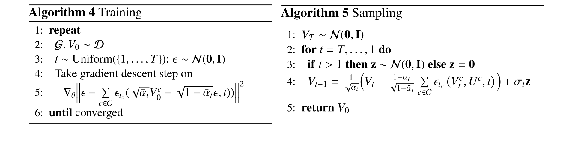
Complete original algorithm group.
Equation

Geometric and Physical Constraint Solving with Diffusion-CCSP
Shared geometry encoders and constraint-specific pose encoders feed a denoising network for each constraint type. The described object representation uses bounding boxes and translation plus sine/cosine yaw; each factor predicts updates for its participating poses. Fixed variables ignore their predicted updates, while free variables receive contributions from every incident constraint. The formulation permits richer variables, but the robot-packing implementation predicts placement poses and relies on separate grasp enumeration and motion planning for feasibility.
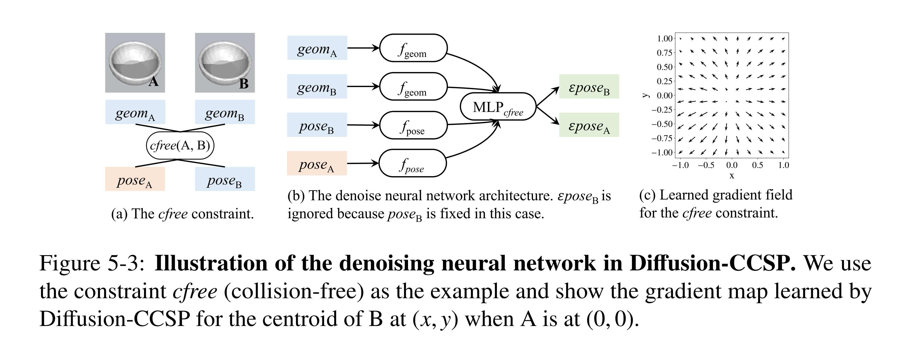
Figure 5-3: Illustration of the denoising neural network in Diffusion-CCSP. We use the constraint cfree (collision-free) as the example and show the gradient map learned by Diffusion-CCSP for the centroid of B at (x, y) when A is at (0, 0).
Equation

Experiments
Four simulated domains compare Langevin-based Diffusion-CCSP with direct reverse diffusion, sequential rejection sampling, and a scene-level StructDiffusion baseline where applicable. Success is measured by actual constraint checks over repeated samples, separating a fixed graph’s solvability from the complete task-and-motion pipeline. Ten-sample main results and extended 100-sample curves expose a speed/success tradeoff; the sequential baseline is capped at 50 attempts per variable.
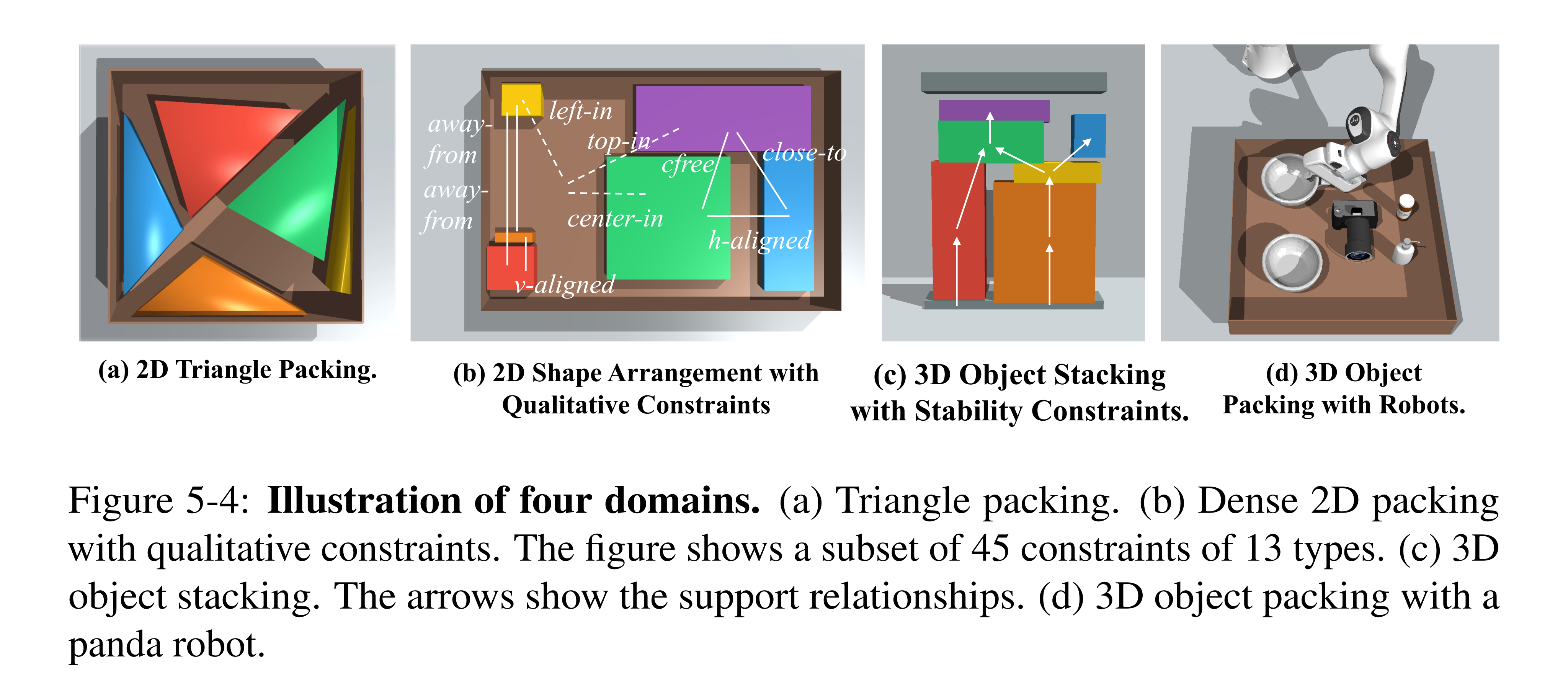
Figure 5-4: Illustration of four domains. (a) Triangle packing. (b) Dense 2D packing with qualitative constraints. The figure shows a subset of 45 constraints of 13 types. (c) 3D object stacking. The arrows show the support relationships. (d) 3D object packing with a panda robot.
2D Triangle Packing
Triangle packing learns from 30,000 tray partitions with two to four triangles and tests transfer to larger sets. Joint sampling handles dense collision/containment constraints better than sequential rejection. StructDiffusion performs similarly and generalizes better in this domain, so the modular solver is not uniformly superior to a transformer that models the whole scene.
2D Shape Arrangement with Qualitative Constraints
Rectangle arrangement adds eleven qualitative relation types to containment and collision constraints. Models train on 30,000 problems with two to four objects and transfer to more densely constrained scenes; Diffusion-CCSP outperforms rejection and its reverse-only variant. The text’s stated test-size range and six-object illustration are not fully consistent. Qualitative training labels come from handcrafted spatial tests, not human annotations, and narrow or disconnected valid regions remain difficult.
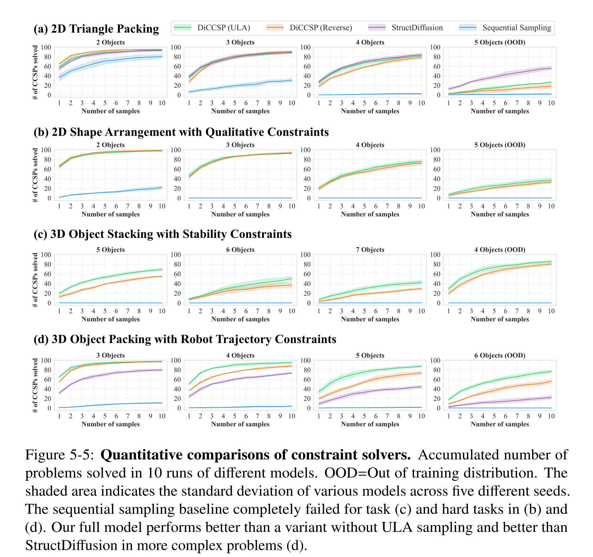
Figure 5-5: Quantitative comparisons of constraint solvers. Accumulated number of problems solved in 10 runs of different models. OOD=Out of training distribution. The shaded area indicates the standard deviation of various models across five different seeds. The sequential sampling baseline completely failed for task (c) and hard tasks in (b) and (d). Our full model performs better than a variant without ULA sampling and better than StructDiffusion in more complex problems (d).
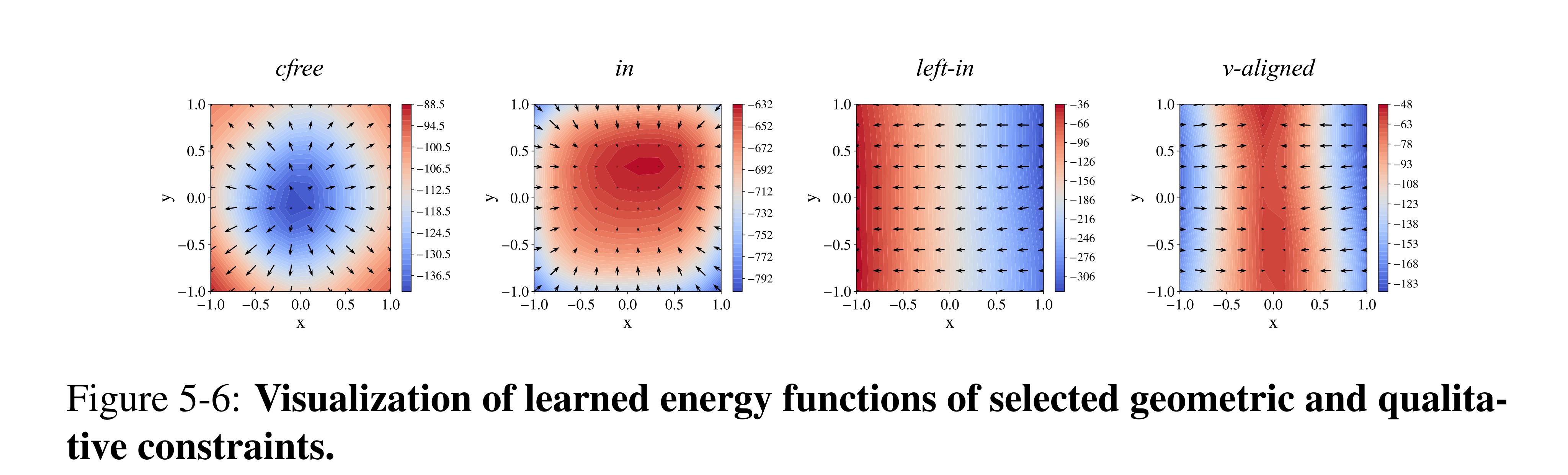
Figure 5-6: Visualization of learned energy functions of selected geometric and qualita- tive constraints.
3D Object Stacking with Stability Constraints
Stacking requires prescribed support relations and physical stability after every placement, including bridge structures with multiple supports. Training uses 24,000 simulated solutions with five to seven objects. An external planner samples placement orders/support structures and calls the continuous solver; failures can therefore reflect an infeasible proposed graph as well as solver failure. Table 5.1 reports 11.9 calls for four objects and 33.33 for five, whereas neighboring prose mentions a different six-box example. Batched per-instance runtimes measure throughput, not complete end-to-end planning latency.
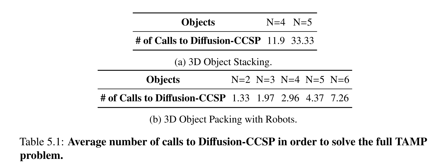
Table 5.1: Average number of calls to Diffusion-CCSP in order to solve the full TAMP problem.
Object Packing with Robot Trajectory Constraints
Robot packing uses a simulated Panda arm and 53 object assets, including objects restricted to side grasps. Training covers three to five objects and testing extends to six. The diffusion model generates promising placements conditioned on geometry and selected grasps; a separate motion planner checks trajectories. Composed constraints outperform rejection and StructDiffusion on larger instances, with mean full-pipeline solver calls increasing to 7.26 for six objects. The paragraph’s reference to “6-triangle packing” appears misplaced, so its numerical claim is not reinterpreted as a clean robot-specific result.
Related Work
The method connects geometric rearrangement, compositional energy/diffusion models, and task and motion planning. Compared with one global scene constraint, factor-specific models support new combinations over different subsets of variables. Generality is a representational aim; the evaluated implementation still depends on a known constraint vocabulary and domain-specific data/checkers.
Discussion
Modular diffusion models provide a practical sampler for new combinations of familiar fixed-arity constraints and can support a search-based planner. Failures and repeated sampling remain, and formal feasibility is delegated to downstream checks. Variable-arity constraints, richer shape representations, real-world training data, and partial observability are future directions rather than demonstrated capabilities.
II Neuro-Symbolic Visual Concepts
Part II develops visual concepts that combine learned perceptual grounding with executable semantics: joint concept learning from questions, rapid acquisition using metaconcepts, cross-domain reasoning through first-order logic, and grammar-based discovery of a grounded lexicon.
Visual Concept Learning
The Neuro-Symbolic Concept Learner (NS-CL) jointly learns object attributes, relations, and question-to-program mappings from image–question–answer examples. An object-centered perception module and a semantic parser communicate through a differentiable executor with fixed logical semantics. The chapter develops work published in Mao et al. (2019).
Introduction
Learning begins with simple object questions and progresses to relations and compositional reasoning. Symbolic programs expose intermediate object selections, while learned concept embeddings connect words to visual features. The goal is to learn grounding and parsing without concept-class or program-trace labels; this does not remove the detector pretraining and supplied language primitives described later.
Related Work
Unlike feature-manipulation or attention-only reasoning, NS-CL executes explicit programs on object features. NS-VQA uses annotated scenes and program supervision; NS-CL instead trains its grounding through answer supervision and differentiable execution. A fixed executor supplies reasoning operations that purely neural baselines must learn, so the comparison includes a substantial architectural prior.
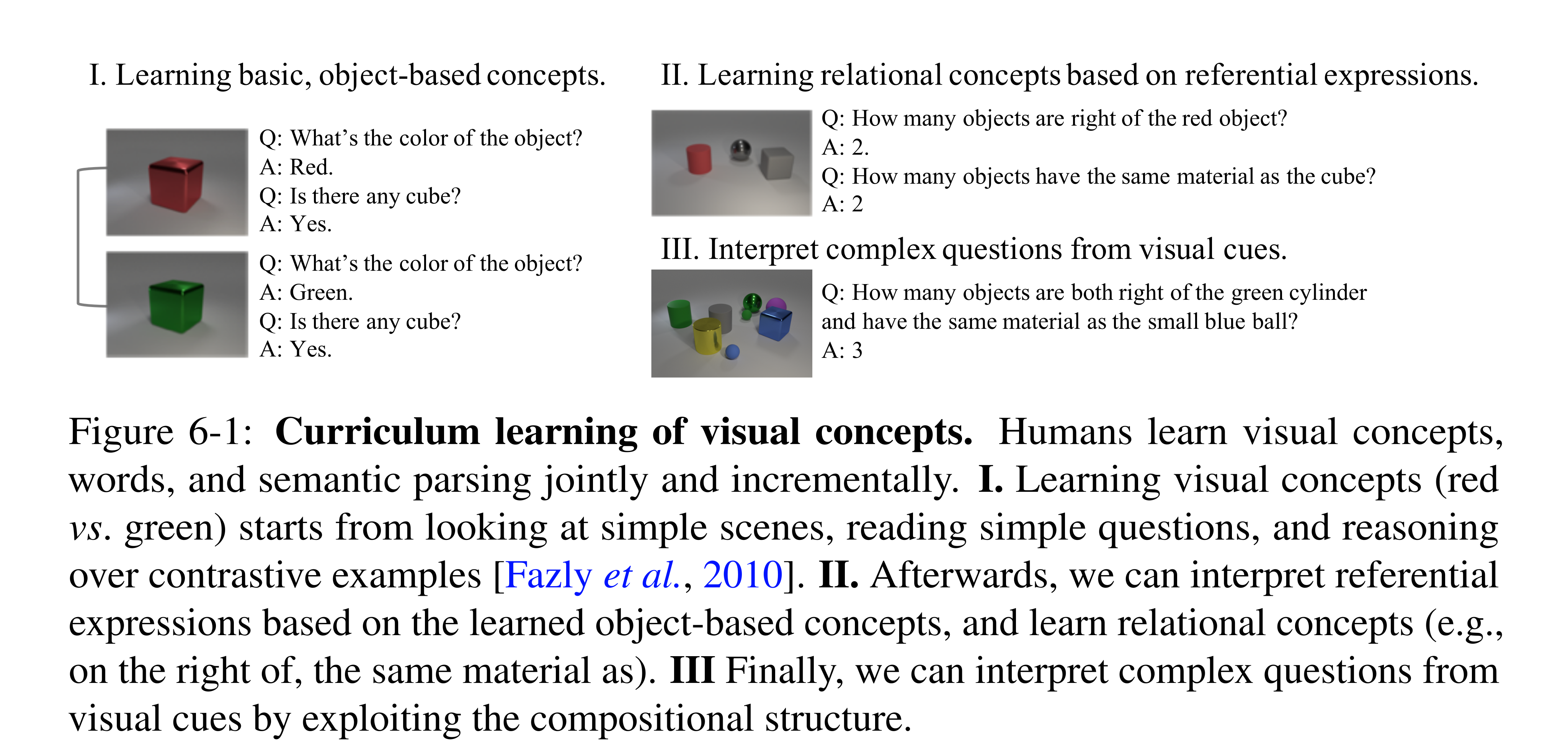
Figure 6-1: Curriculum learning of visual concepts. Humans learn visual concepts, words, and semantic parsing jointly and incrementally. I. Learning visual concepts (red vs. green) starts from looking at simple scenes, reading simple questions, and reasoning over contrastive examples [Fazly et al., 2010]. II. Afterwards, we can interpret referential expressions based on the learned object-based concepts, and learn relational concepts (e.g., on the right of, the same material as). III Finally, we can interpret complex questions from visual cues by exploiting the compositional structure.
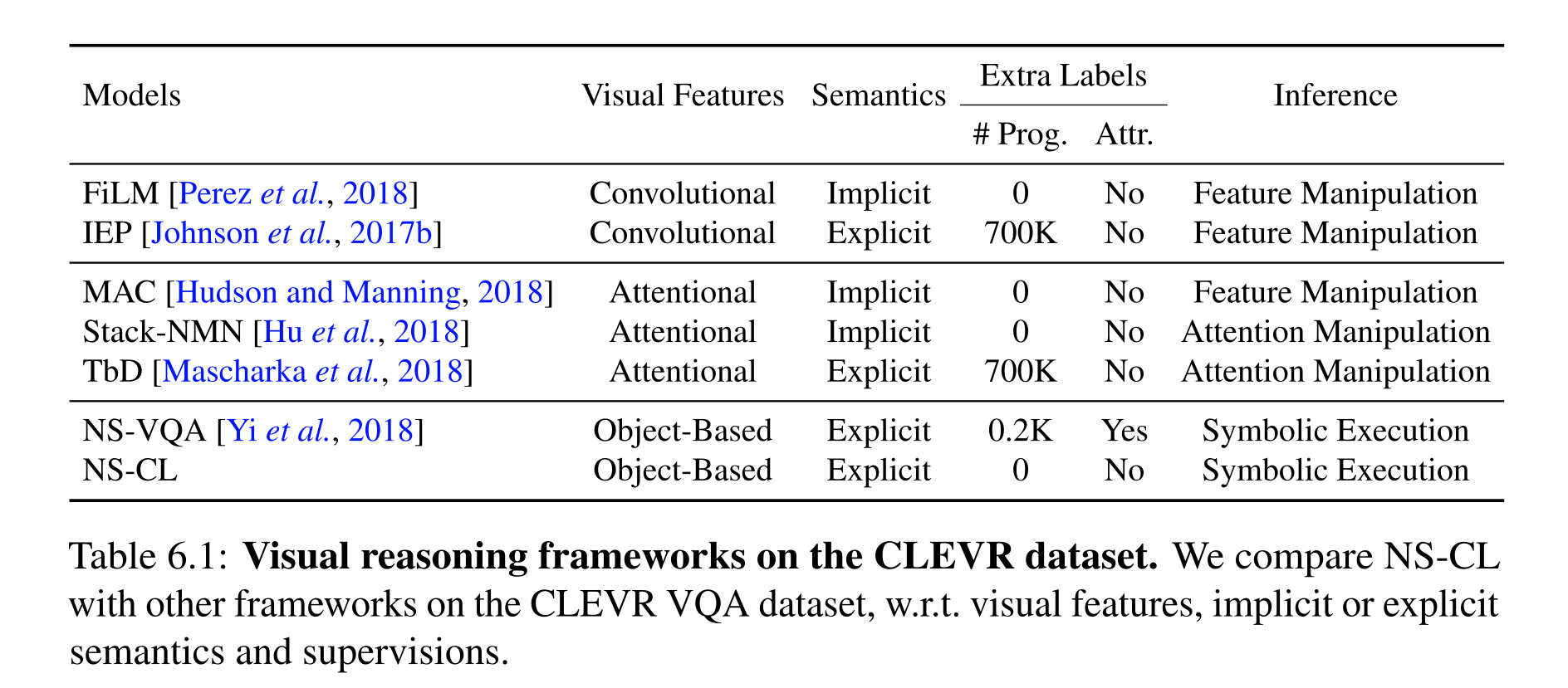
Table 6.1: Visual reasoning frameworks on the CLEVR dataset. We compare NS-CL with other frameworks on the CLEVR VQA dataset, w.r.t. visual features, implicit or explicit semantics and supervisions.
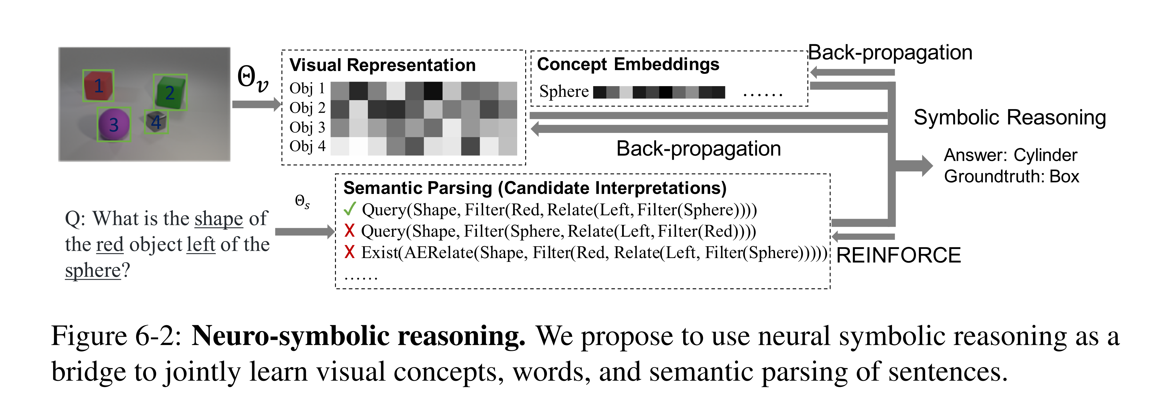
Figure 6-2: Neuro-symbolic reasoning. We propose to use neural symbolic reasoning as a bridge to jointly learn visual concepts, words, and semantic parsing of sentences.
Neuro-Symbolic Concept Learner
Perception detects objects and represents them with latent features. A sequence-to-tree parser produces a program in a predefined domain-specific language; deterministic modules execute it using soft object sets. Answer loss updates the visual and concept representations, while program search/reinforcement learning trains the discrete parser.
Model details
A pretrained Mask R-CNN proposes boxes. ResNet-34 features combine each region with whole-scene context, which supports relative size and spatial relations. Attribute-specific operators map features into embedding spaces; cosine similarity to learned concept vectors yields soft classifications. Pairwise features ground relations.
A bidirectional GRU encodes the question, and a recursive decoder selects operations and concept parameters. The executor represents an object set by membership scores and composes filtering, relations, set operations, counting, and attribute queries. These scores permit differentiation; a transparent execution trace does not guarantee that its learned grounding is correct.
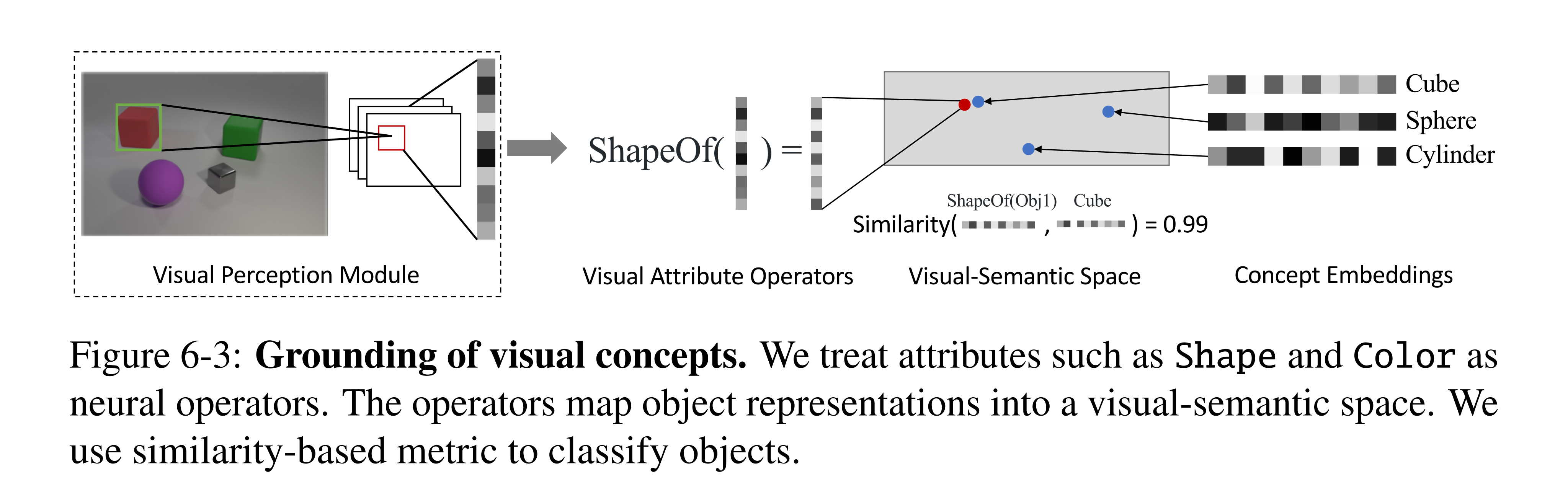
Figure 6-3: Grounding of visual concepts. We treat attributes such as Shape and Color as neural operators. The operators map object representations into a visual-semantic space. We use similarity-based metric to classify objects.
Training paradigm
The objective rewards the correct answer averaged over parser-produced programs. Grounding parameters receive gradients through execution; the parser uses REINFORCE and off-policy search for answer-consistent programs. Training proceeds from object concepts to relations, then complex parsing with perception temporarily frozen, followed by joint fine-tuning. Appendix F groups the last two phases into one of three lessons.
Equation

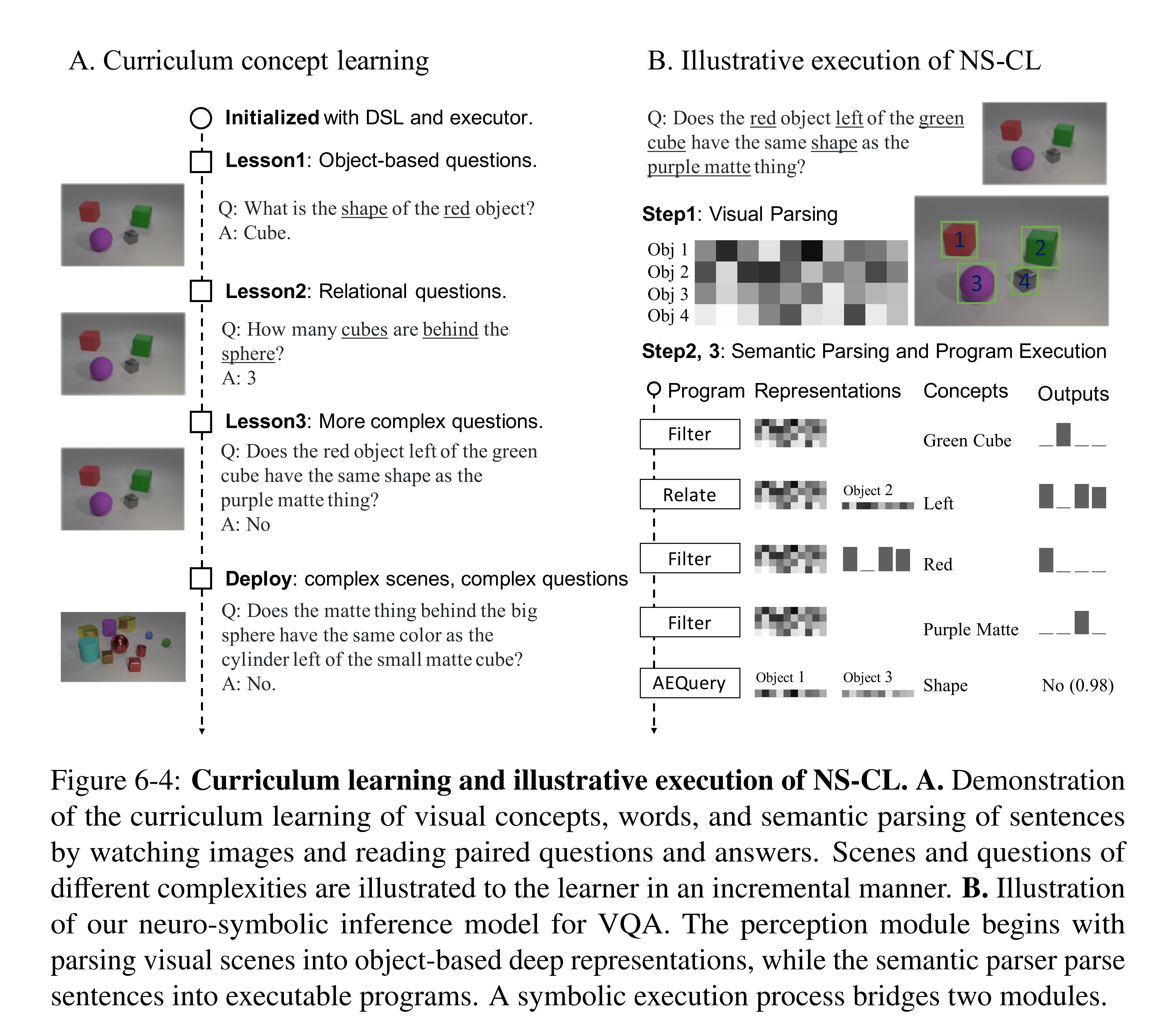
Figure 6-4: Curriculum learning and illustrative execution of NS-CL. A. Demonstration of the curriculum learning of visual concepts, words, and semantic parsing of sentences by watching images and reading paired questions and answers. Scenes and questions of different complexities are illustrated to the learner in an incremental manner. B. Illustration of our neuro-symbolic inference model for VQA. The perception module begins with parsing visual scenes into object-based deep representations, while the semantic parser parse sentences into executable programs. A symbolic execution process bridges two modules.
Experiments
The main CLEVR setup trains on 5,000 images with 20 generated questions per image. The detector is separately pretrained on 4,000 generated CLEVR images with bounding-box annotations, and the feature extractor uses ImageNet pretraining. Thus “no extra labels” applies to concept/program learning rather than every component of the complete pipeline.
Visual concept learning
Learned object properties classify at roughly 99% accuracy; spatial relations are weaker because their supervision is indirect. On diagnostic concept-counting questions, NS-CL averages 98.7%, versus IEP 90.6%, MAC 95.9%, and high-resolution TbD 96.5%. This supports grounded concept accuracy in the synthetic domain, not unrestricted visual recognition.
Data-efficient and interpretable visual reasoning
Table 6.4 gives 98.9% overall CLEVR accuracy with zero program annotations, tying MAC’s displayed overall score and approaching TbD’s 99.1% with full program supervision. The data-efficiency study reports 98.9% at its 10%-data setting and 99.2% with the full training set. Simply supplying object features to TbD/MAC does not reproduce these results, although mask-guided attention speeds training.
The reported parser score above 99.9% evaluates answers from execution on annotated object scenes, rather than exact syntax recovery; equivalent programs are allowed. ImageNet and detector pretraining, the supplied DSL, and curriculum remain relevant sources of prior knowledge.
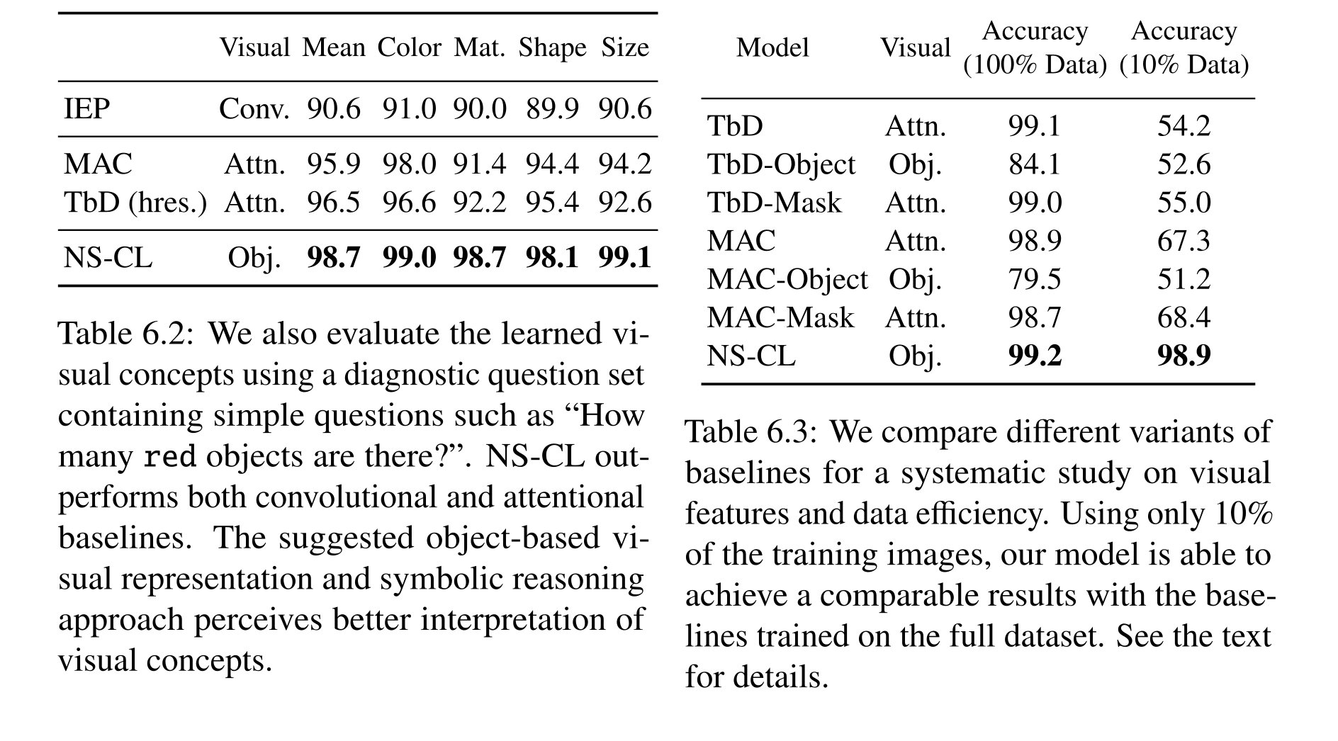
Table 6.2: We also evaluate the learned vi- sual concepts using a diagnostic question set containing simple questions such as “How many red objects are there?”. NS-CL out- performs both convolutional and attentional baselines. The suggested object-based vi- sual representation and symbolic reasoning approach perceives better interpretation of visual concepts.
Table 6.3: We compare different variants of baselines for a systematic study on visual features and data efficiency. Using only 10% of the training images, our model is able to achieve a comparable results with the base- lines trained on the full dataset. See the text for details.
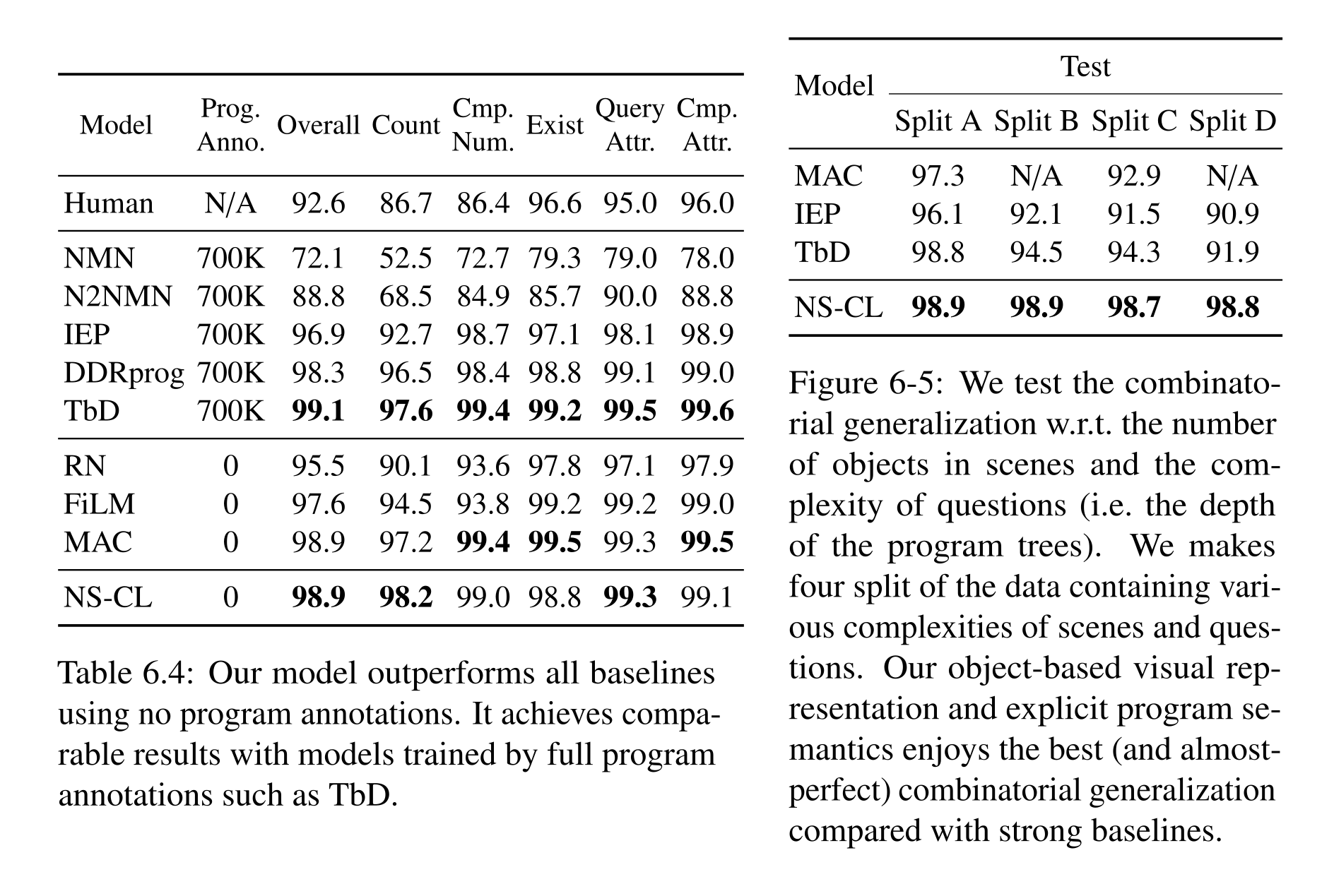
Table 6.4: Our model outperforms all baselines using no program annotations. It achieves compa- rable results with models trained by full program annotations such as TbD.
Figure 6-5: We test the combinato- rial generalization w.r.t. the number of objects in scenes and the com- plexity of questions (i.e. the depth of the program trees). We makes four split of the data containing vari- ous complexities of scenes and ques- tions. Our object-based visual rep- resentation and explicit program se- mantics enjoys the best (and almost- perfect) combinatorial generalization compared with strong baselines.
Generalization to new attributes and compositions
For CLEVR-CoGenT, attribute operators are pretrained and frozen while concept embeddings and parsing learn from split A; accuracy is 98.8% on A and 98.9% on the color–shape-swapped B. This result depends on those pretrained attribute operators, since direct training on A otherwise entangles color with shape.
For a novel purple concept, models first train without purple and adapt on 100 images containing it. NS-CL reaches 93.9% QA accuracy, ahead of IEP and TbD by 4.6 and 6.1 points. All methods in this experiment use a semantic parser pretrained on full CLEVR, so the adaptation test primarily isolates visual concept acquisition.
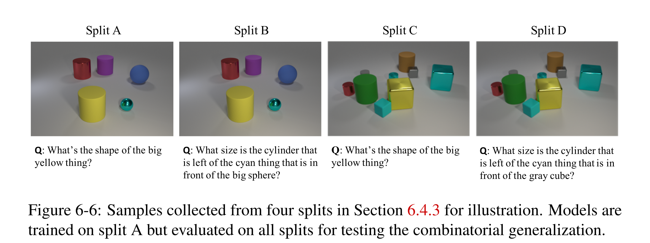
Figure 6-6: Samples collected from four splits in Section 6.4.3 for illustration. Models are trained on split A but evaluated on all splits for testing the combinatorial generalization.
Combinatorial generalization to new scenes and questions
Train on scenes with fewer than six objects and programs shallower than five, then test larger scenes and/or deeper questions. NS-CL remains at 98.7–98.9% across the four splits, while the listed alternatives degrade. Explicit-program methods use a parser pretrained on the full dataset, and count queries over more than six objects are removed for comparison. This demonstrates execution/perception composition under that protocol, not fully unseen language parsing.
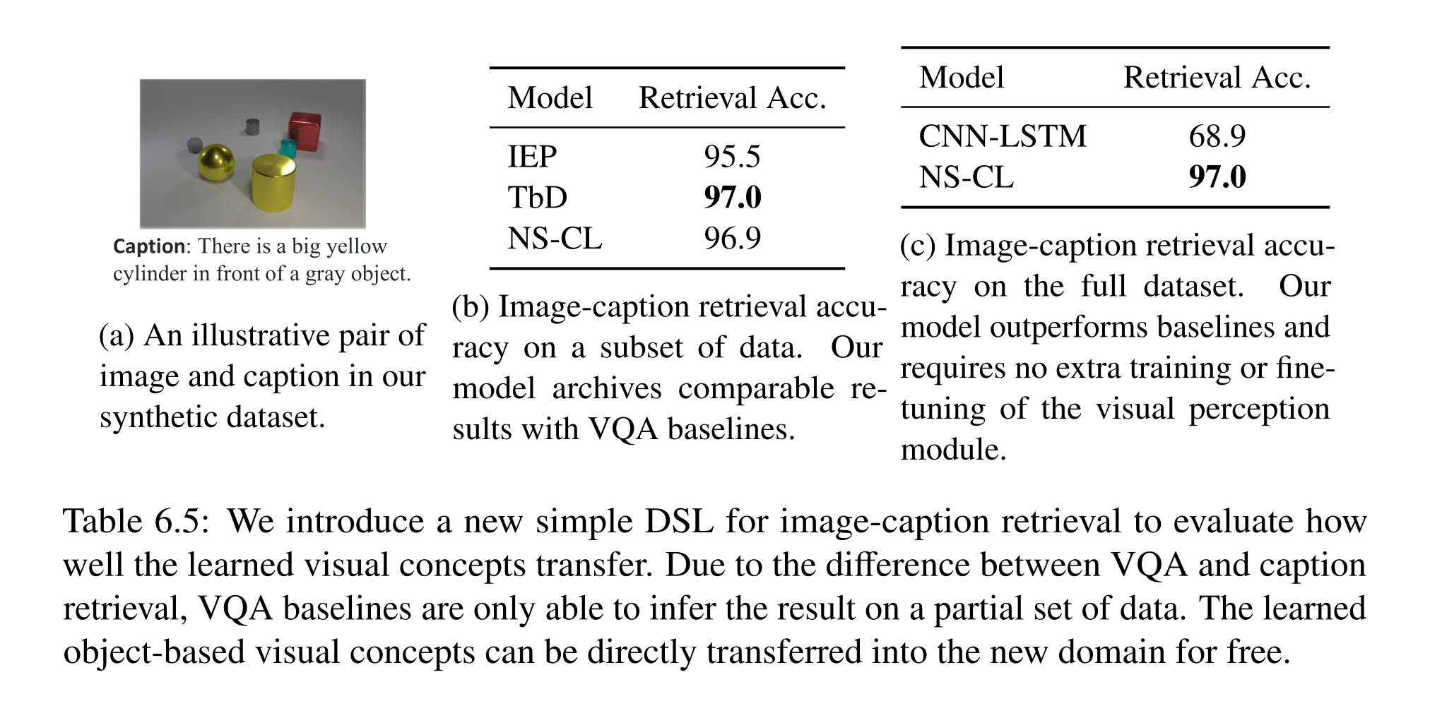
Table 6.5: We introduce a new simple DSL for image-caption retrieval to evaluate how well the learned visual concepts transfer. Due to the difference between VQA and caption retrieval, VQA baselines are only able to infer the result on a partial set of data. The learned object-based visual concepts can be directly transferred into the new domain for free.
Extending to other program domain
Learned visual concepts transfer to a new retrieval DSL while only a new caption parser is trained. Retrieval here means deciding whether an image contains a caption’s relational triple, rather than open-ended ranked search. On the unambiguous subset, NS-CL scores 96.9% versus TbD 97.0%; on the full synthetic dataset it scores 97.0% versus CNN-LSTM 68.9%. The gain on the full task is 28.1 percentage points, rounded to “30%” in the source.
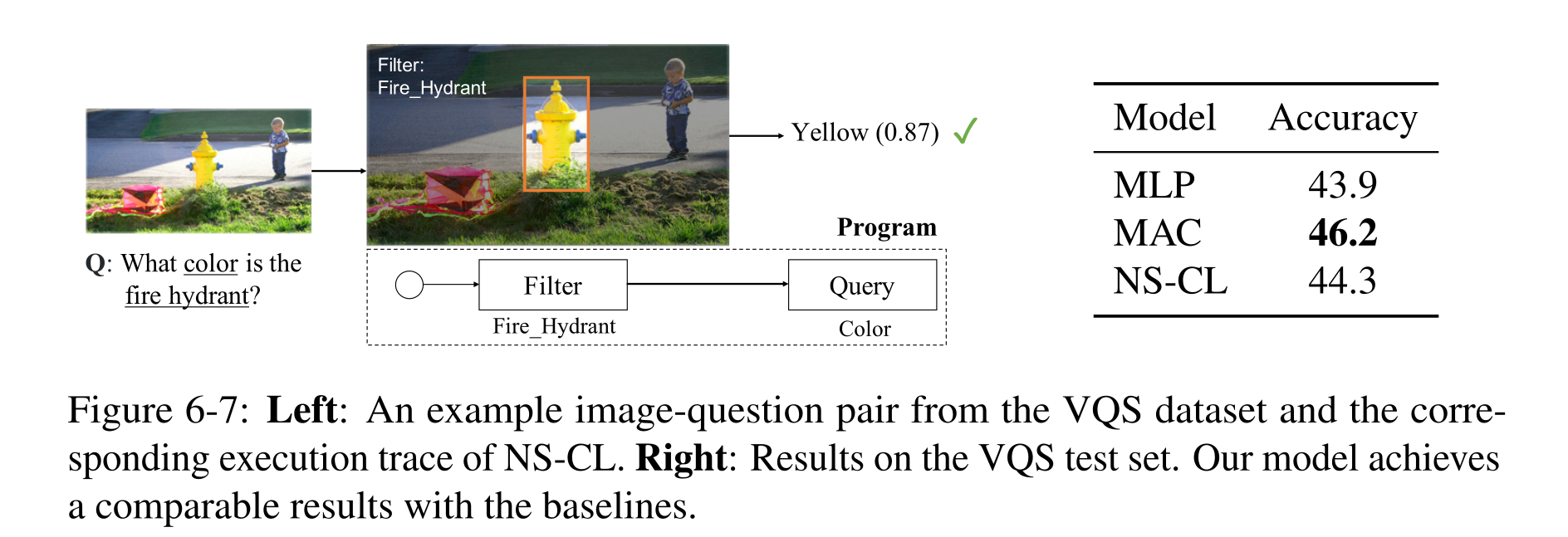
Figure 6-7: Left: An example image-question pair from the VQS dataset and the corre- sponding execution trace of NS-CL. Right: Results on the VQS test set. Our model achieves a comparable results with the baselines.
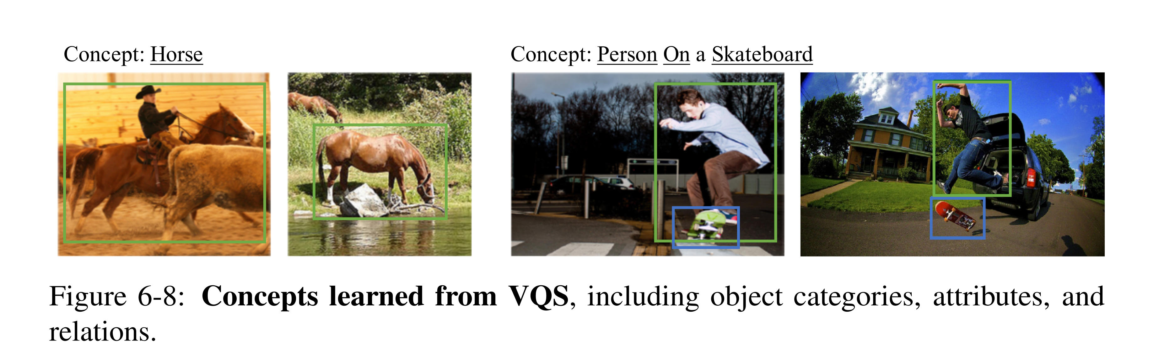
Figure 6-8: Concepts learned from VQS, including object categories, attributes, and relations.
Extending to natural images and language
On grounded VQS questions over MS-COCO images, a pretrained dependency parser supplies programs and COCO/ImageNet models supply proposals/features. NS-CL reaches 44.3%, versus MLP 43.9% and MAC 46.2%, in the 18-choice evaluation detailed in Appendix F. This establishes feasibility with interpretable traces, not a lead on unrestricted natural-image VQA. Events and activities remain outside the demonstrated static-concept scope.

Discussion
NS-CL separates concept learning from fixed compositional execution, enabling data efficiency and reuse across selected visual tasks. Its limits are a predefined primitive language and supplied concept-word inventory. Richer control flow increases expressiveness but complicates differentiable learning; later chapters address concept discovery through LLM interpretation and grounded grammar learning.
Fast Visual Concept Learning with Metaconcepts
FALCON learns a reusable visual-concept representation from a few image–description examples and sentences relating the new concept to known ones. A learned concept library supports later recognition and compositional questions; this chapter, based on Mei et al. (2022), studies fast concept acquisition rather than training a new question-answering network for each concept.
Introduction
A purple cylinder alone cannot reveal whether a new word names its color or shape. Supplemental statements such as “purple and yellow are colors” constrain this ambiguity through known concepts. FALCON grounds the examples, combines their visual evidence with concept relationships, and adds an embedding to a growing library. Its evaluations use annotated images and generated language, with pretrained perception and semantic parsing.
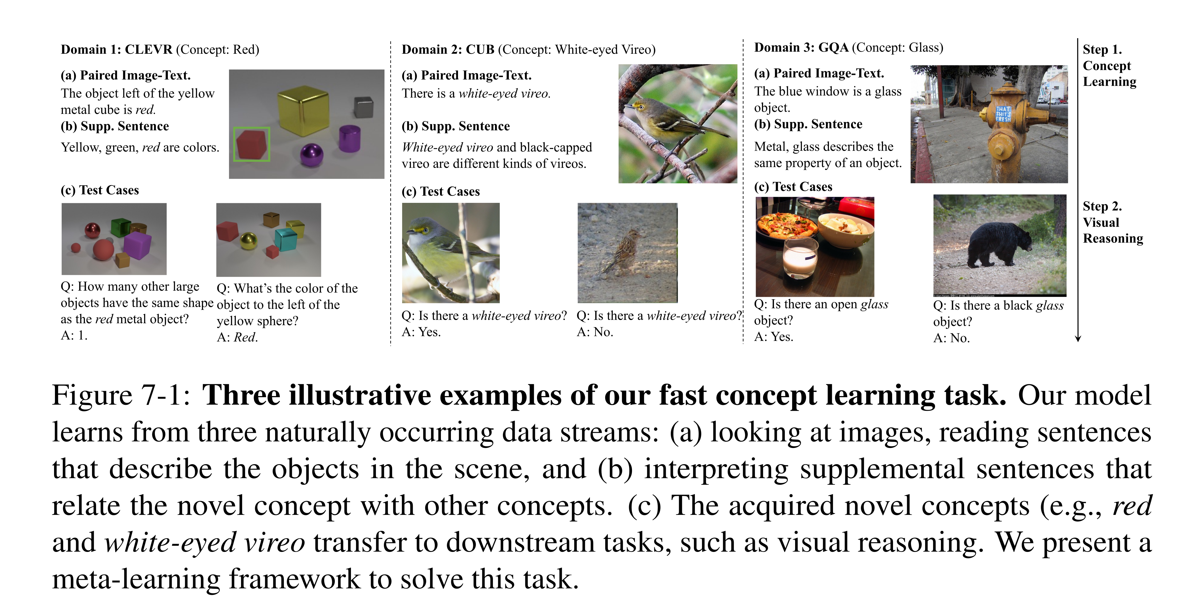
Figure 7-1: Three illustrative examples of our fast concept learning task. Our model learns from three naturally occurring data streams: (a) looking at images, reading sentences that describe the objects in the scene, and (b) interpreting supplemental sentences that relate the novel concept with other concepts. (c) The acquired novel concepts (e.g., red and white-eyed vireo transfer to downstream tasks, such as visual reasoning. We present a meta-learning framework to solve this task.
FALCON
Each learning task supplies a novel concept, image–description examples, supplemental concept relations, and downstream questions. Existing concepts identify the example objects; a graph or recurrent meta-learner predicts the new embedding, which the same differentiable executor can subsequently use. Learning and question answering are separated by this persistent concept representation.
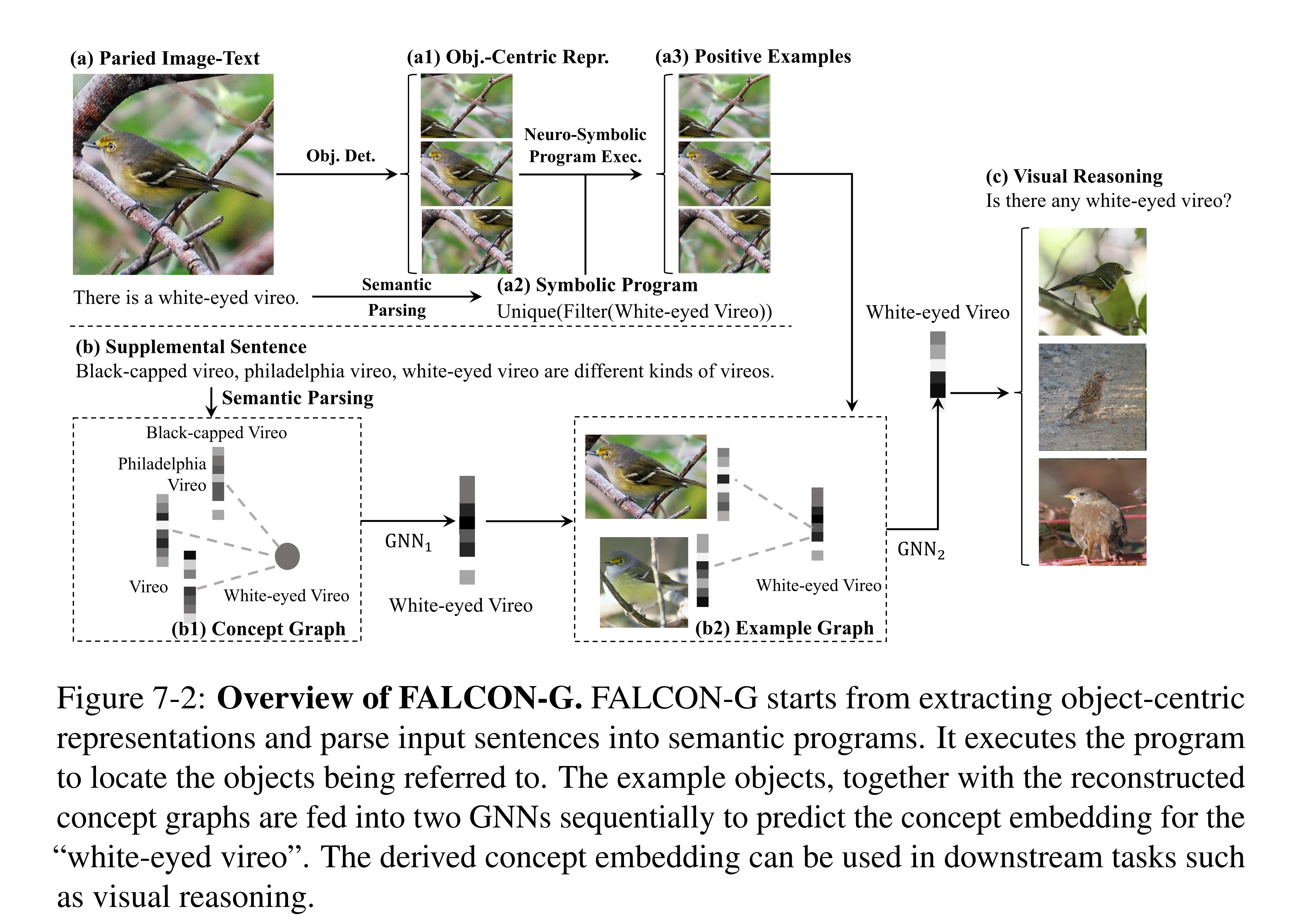
Figure 7-2: Overview of FALCON-G. FALCON-G starts from extracting object-centric representations and parse input sentences into semantic programs. It executes the program to locate the objects being referred to. The example objects, together with the reconstructed concept graphs are fed into two GNNs sequentially to predict the concept embedding for the “white-eyed vireo”. The derived concept embedding can be used in downstream tasks such as visual reasoning.
Visual Representations and Embedding Spaces
Mask-RCNN proposals and ResNet-34 features represent objects and object pairs. Concepts are axis-aligned boxes in a 100-dimensional unit domain; objects are nearly point-sized boxes. Intersection volume relative to the object box scores membership, while containment represents asymmetric concept entailment. Smooth positive-part functions make box volumes differentiable. Hyperplane and hypercone alternatives provide comparison representations; box geometry is an inductive bias, not an enforced logical guarantee.
Neuro-Symbolic Reasoning
Pretrained parsers translate descriptions, supplemental relationships, and questions into symbolic structures. The differentiable executor follows the NS-CL operator design, applying learned concept-membership scores to soft object sets. Descriptions first select examples using known concepts, and questions can then reuse the new concept within relational, counting, or existence programs. Correct execution still depends on detection, parsing, and visual grounding.
Learning to Learn Concepts
The learner samples candidate embeddings from a learned prior and updates them using known-concept relationships and visual examples. FALCON-G applies graph networks; FALCON-R processes randomized relation sequences recurrently. Candidates are ranked by how well they explain the positive examples. Downstream answer loss trains the meta-learner, with a prior regularizer discouraging implausible embeddings; it does not directly enforce every supplied relation as a hard constraint.
Equation

Training and Testing Paradigm
Training first learns perception and base concepts, then meta-trains novel-concept inference while keeping the base library fixed. Validation and test concepts are held out from concept training. In the continual variant, previously inferred concepts become available to later learning tasks. This tests sequential expansion of the library, with frozen earlier embeddings, rather than establishing resistance to every form of long-term forgetting.
Experiments
Experiments compare graph and recurrent inference, three embedding spaces, and end-to-end or concept-centric baselines on CUB birds, CLEVR, and GQA. The central comparisons separate visual examples alone from examples supplemented by concept relations. Reported accuracies depend on generated question distributions and each dataset’s concept split.
Dataset
CUB splits 200 species into 100/50/50 training, validation, and test species, producing 211/83/72 taxonomic concepts; each novel concept receives one image. CLEVR holds out colors and a shape across four splits, and GQA splits 105 frequent concepts into 89/6/10. Supplemental relations include hypernyms and shared attributes. CUB evaluation uses generated binary questions about a single bird, not 200-way species classification.
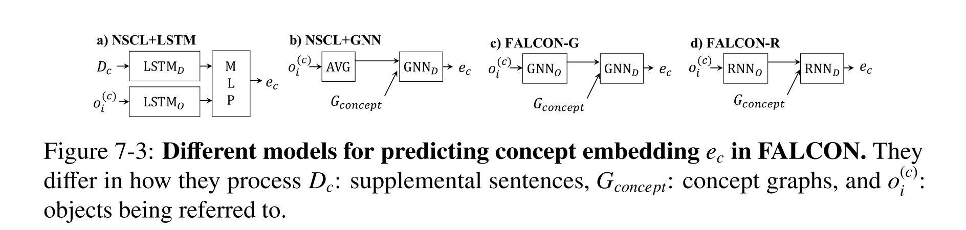
Figure 7-3: Different models for predicting concept embedding ec in FALCON. They differ in how they process Dc: supplemental sentences, Gconcept: concept graphs, and o(c) i : objects being referred to.
Baseline
CNN+LSTM and MAC process the task inputs end to end. NSCL+LSTM and NSCL+GNN instead infer a concept embedding for a shared executor; FALCON adds learned candidate inference using separate evidence sources. Box embeddings have 100 dimensions with center/size parameters, whereas hyperplane and hypercone embeddings use 512 dimensions. These comparisons therefore change both geometry and representation size.
Results on CUB
Table 7.1 gives the best CUB result to FALCON-G with boxes (81.33%), followed by FALCON-R (79.83%); the surrounding sentence naming R as best disagrees with the table. Without supplemental relations, G scores 76.37%, and continual learning scores 79.67%. Fewer base concepts reduce performance, while even 25% of related concepts supplies much of the observed benefit. FALCON is not best under every alternative geometry, so the strongest result concerns the box-based configuration.
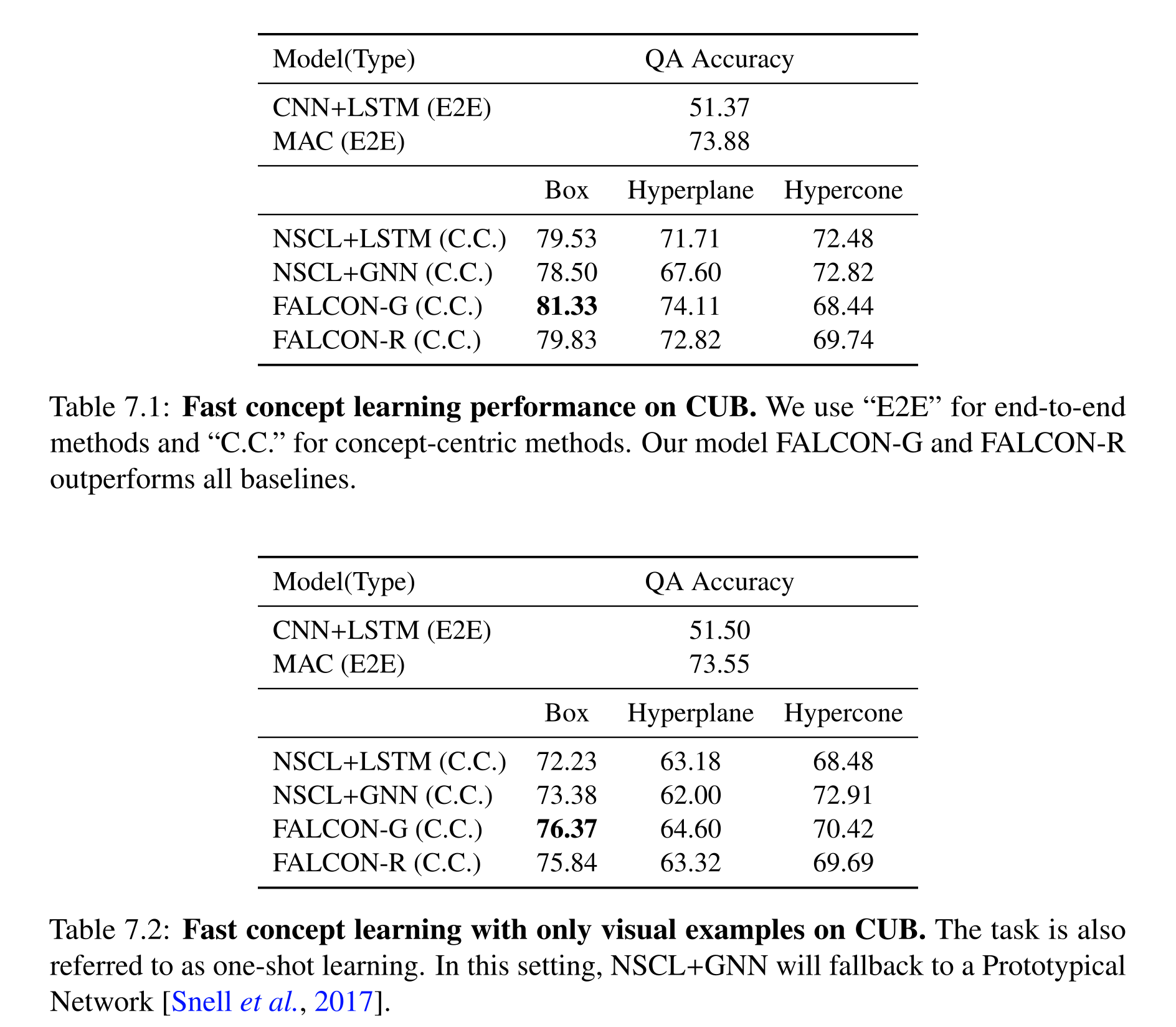
Table 7.1: Fast concept learning performance on CUB. We use “E2E” for end-to-end methods and “C.C.” for concept-centric methods. Our model FALCON-G and FALCON-R outperforms all baselines.
Table 7.2: Fast concept learning with only visual examples on CUB. The task is also referred to as one-shot learning. In this setting, NSCL+GNN will fallback to a Prototypical Network [Snell et al., 2017].
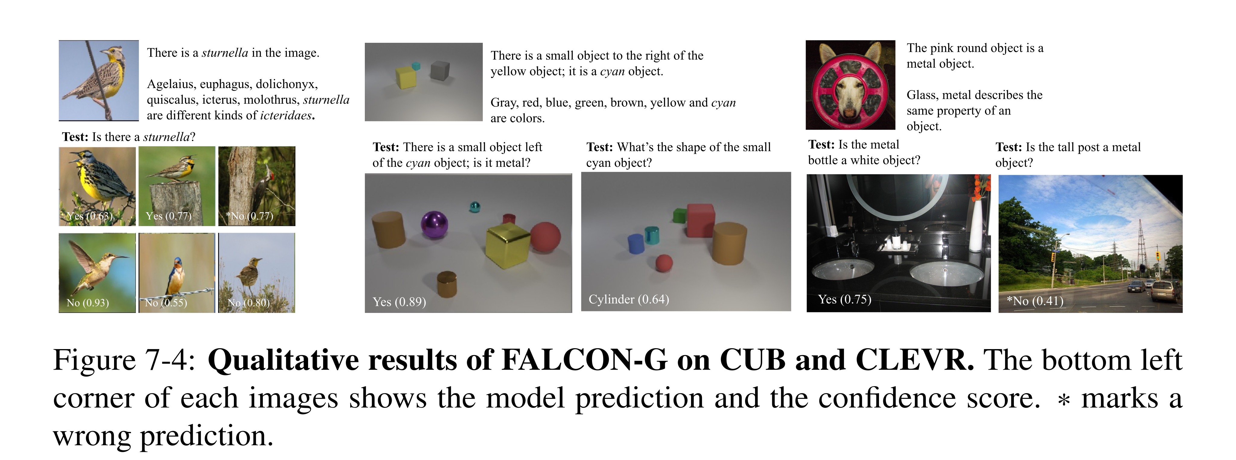
Figure 7-4: Qualitative results of FALCON-G on CUB and CLEVR. The bottom left corner of each images shows the model prediction and the confidence score. * marks a wrong prediction.
Results on CLEVR
On CLEVR, supplemental concept relations raise FALCON-G from 68.47% to 88.40%, compared with NSCL+GNN’s 65.01% to 84.11%. The benefit is pronounced when an example has several plausible attributes. Biased examples make this explicit by pairing every novel cylinder with purple: Appendix Table G.7 reports 87.29% for G with supplemental information, whereas the chapter text states 88.29%.
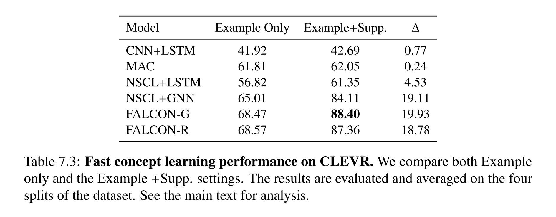
Table 7.3: Fast concept learning performance on CLEVR. We compare both Example only and the Example +Supp. settings. The results are evaluated and averaged on the four splits of the dataset. See the main text for analysis.
Results on GQA
On GQA, FALCON-G with boxes reaches 55.96%, versus 55.41% for NSCL+LSTM and 54.99% for MAC. The gains are much smaller than on CLEVR, reflecting harder natural-image grounding and more complex concept boundaries. The reported point estimates have no accompanying uncertainty analysis; they support a modest advantage in this benchmark, not a large general improvement.
Related Work
The approach joins few-shot learning, meta-learning, concept representations, and neuro-symbolic reasoning. Unlike methods that only classify examples by similarity, it uses linguistic relations to constrain a reusable concept embedding. Box embeddings offer an asymmetric containment structure for entailment, while the symbolic executor composes learned concepts into questions.
Discussion
Fast concept learning benefits from combining grounded examples with knowledge about relations among concepts. The resulting library can support recognition, reasoning, and later concept acquisition. The demonstrated setting nevertheless assumes a concept vocabulary, generated language, pretrained modules, and a restricted family of concept representations; broader language and visual ambiguity remain unresolved.
Concept Learning Across Domains and Modalities
LEFT combines an LLM that translates language into first-order logic, a differentiable executor shared across domains, and trainable domain-specific grounding modules. Based on Hsu et al. (2023), the chapter extends NS-CL-style concept learning to images, 3D point clouds, human motion, and manipulation. The shared component is the reasoning framework; perception and concept groundings still depend on the modality and its training data.
Introduction
A symbol such as “left” supports related reasoning across domains while requiring different perceptual groundings. Inference-only systems depend on available pretrained APIs, which may not cover a new modality. LEFT instead learns the grounding modules through a differentiable logic executor, while an LLM resolves language into programs. This separates reusable reasoning structure from the data-dependent interpretation of concepts.
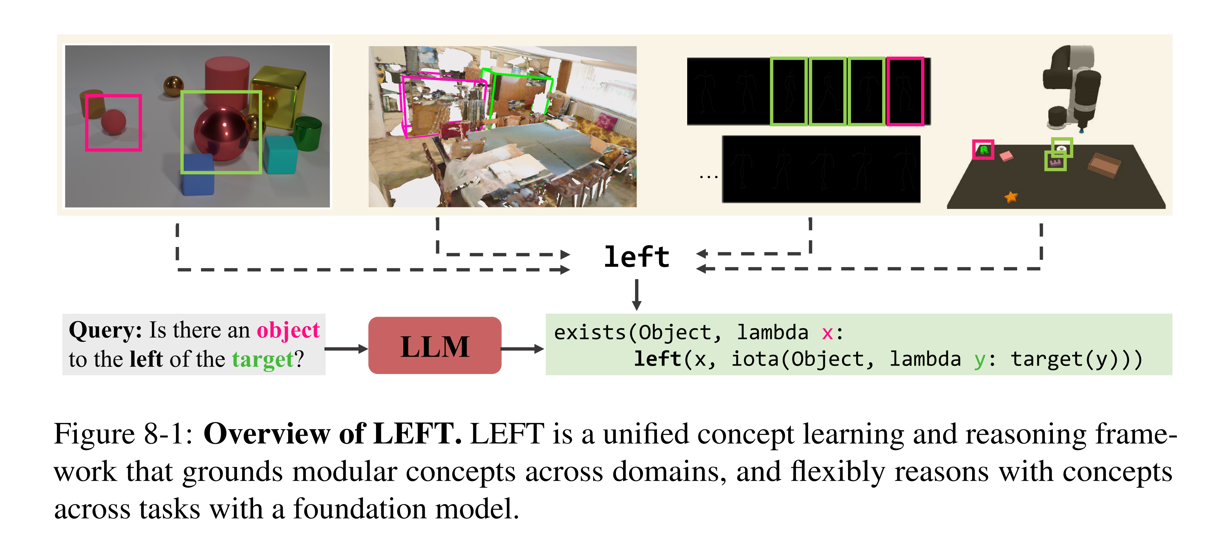
Figure 8-1: Overview of LEFT. LEFT is a unified concept learning and reasoning frame- work that grounds modular concepts across domains, and flexibly reasons with concepts across tasks with a foundation model.
Logic-Enhanced Foundation Model (LEFT)
The LLM interpreter generates hierarchical logic programs; a recursive tensor-based executor evaluates them; modality-specific encoders and concept networks supply predicate scores. Concept names and arities produced by the interpreter determine which grounding modules are initialized. Automatic initialization supplies an architecture, not an already learned meaning for an arbitrary new predicate.
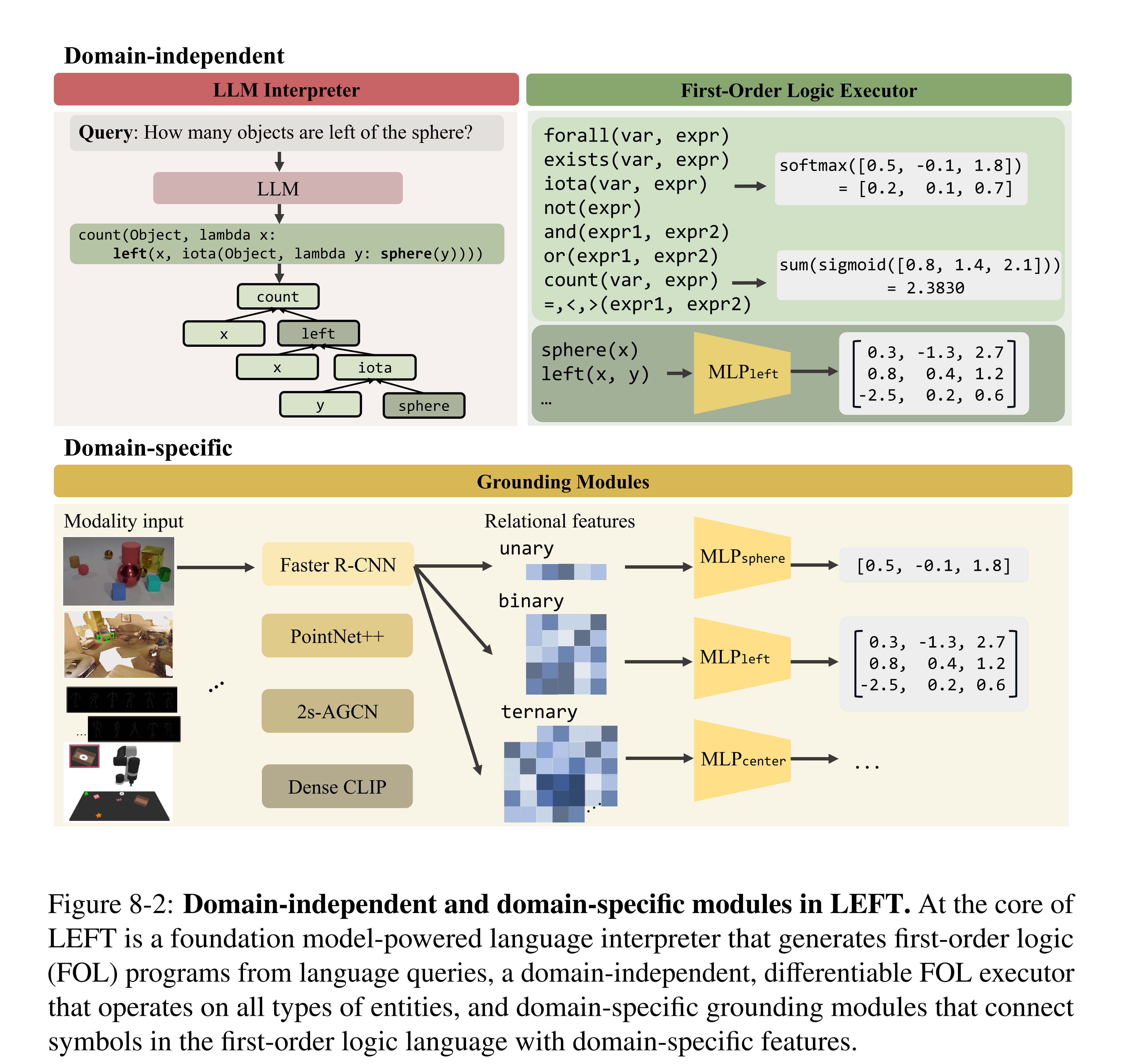
Figure 8-2: Domain-independent and domain-specific modules in LEFT. At the core of LEFT is a foundation model-powered language interpreter that generates first-order logic (FOL) programs from language queries, a domain-independent, differentiable FOL executor that operates on all types of entities, and domain-specific grounding modules that connect symbols in the first-order logic language with domain-specific features.
Domain-independent LLM interpreter
GPT-3.5 receives domain-independent syntax instructions and simple examples involving generic objects. It first reasons about and simplifies the query, then emits logic that can express references, analogies, or patterns. The language includes predefined logical and numerical operations together with learned predicates and output functions. This reduces domain-specific program engineering, but parsing errors and non-executable LLM outputs remain possible.
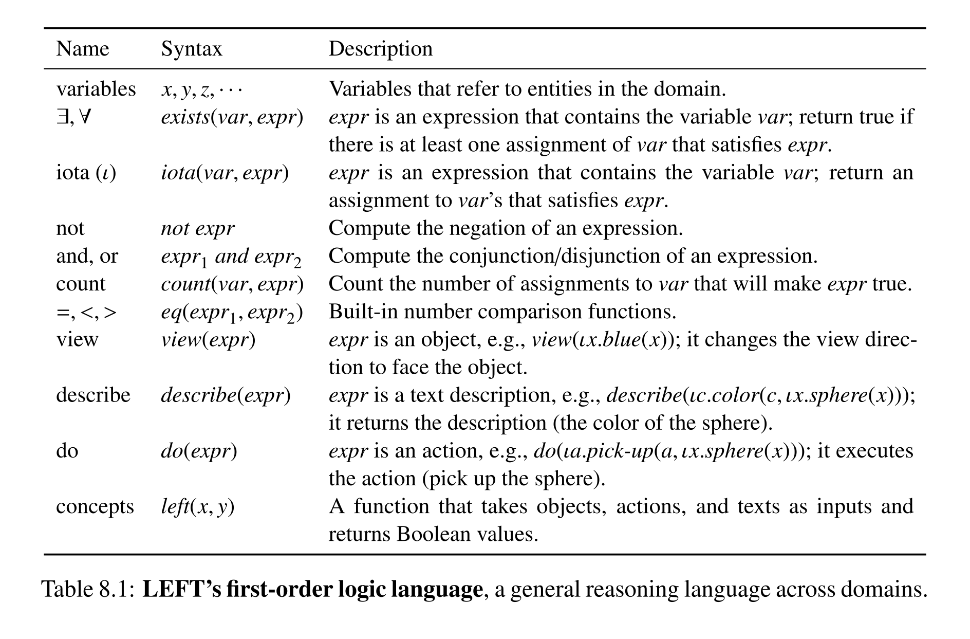
Table 8.1: LEFT’s first-order logic language, a general reasoning language across domains.
Domain-independent first-order logic executor
Predicates are tensors over entities: unary properties form vectors, binary relations form matrices, and higher arities add dimensions. Existential and universal quantifiers use maximum and minimum; conjunction/disjunction use elementwise minimum/maximum; negation changes logit sign; iota uses softmax; counting sums sigmoid memberships. Numerical comparisons use smooth thresholds. These differentiable relaxations enable grounding gradients, but soft selection and counts are not exact discrete logical inference.
Domain-specific grounding modules
Domain encoders include Faster R-CNN or DenseCLIP for images, PointNet++ for point clouds, and 2s-AGCN for motion. An MLP for each named predicate maps unary or relational features to scores, with its input structure determined by arity. Training backpropagates through the executor into these modules. The method avoids hand-coding each concept’s logic while retaining modality-specific encoders, entity representations, and training choices.
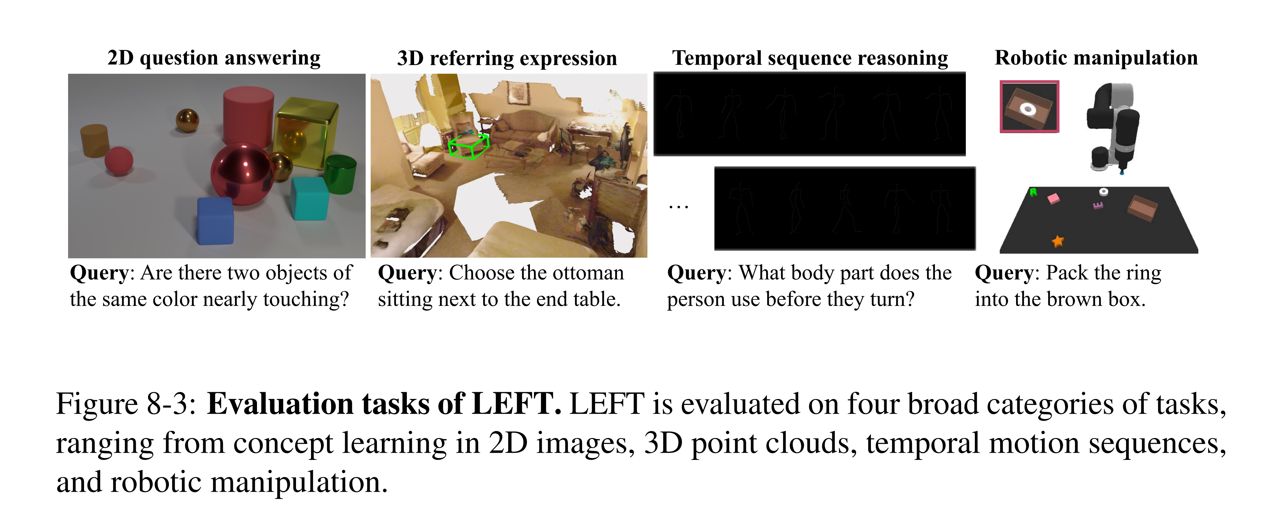
Figure 8-3: Evaluation tasks of LEFT. LEFT is evaluated on four broad categories of tasks, ranging from concept learning in 2D images, 3D point clouds, temporal motion sequences, and robotic manipulation.
Experiments
Six datasets test concept learning in four domains, followed by three CLEVR-derived transfer tasks. Comparisons distinguish task accuracy, reduced-data training, and reuse of trained concepts in unseen reasoning structures. Results therefore test a common framework across separately grounded domains and within-domain reasoning transfer, rather than one zero-shot model for all modalities.
Concept learning across domains
LEFT scores 99.6% on CLEVR, 62.0% on SR3D, 58.2% on HumanMotionQA, and 79.3% reward on the CLIPort packing task, broadly matching specialized neuro-symbolic systems. It does not beat every end-to-end comparison: BUTD’s SR3D score is higher under a constrained class vocabulary. For natural language, executable-query/all-query accuracies are 78.8%/69.8% on CLEVR-Humans and 49.6%/48.5% on the selected NR3D subset. Low-data results favor modular reasoning over the listed end-to-end models, although NS-CL’s additional attribute priors outperform LEFT at 10% CLEVR data (98.9% versus 94.1%).
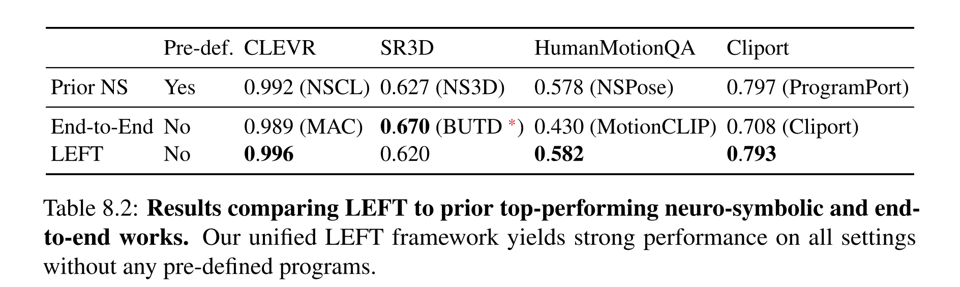
Table 8.2: Results comparing LEFT to prior top-performing neuro-symbolic and end- to-end works. Our unified LEFT framework yields strong performance on all settings without any pre-defined programs.
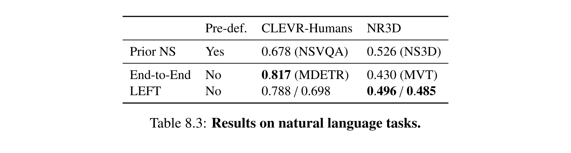
Table 8.3: Results on natural language tasks.
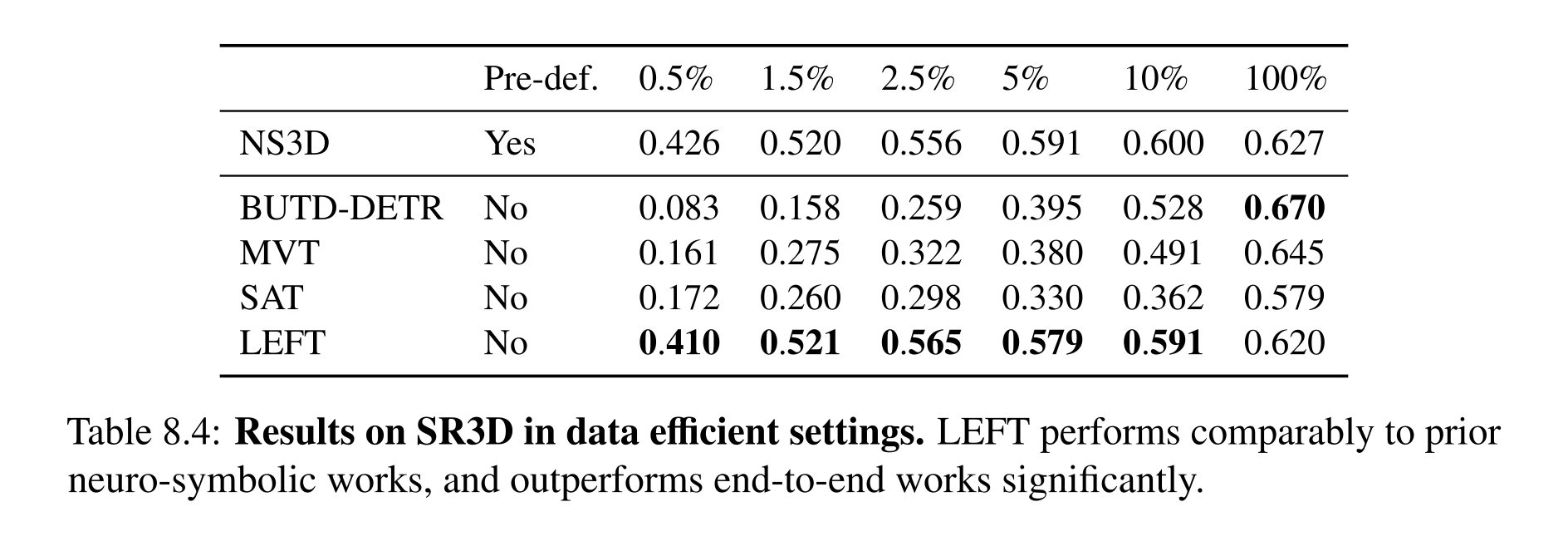
Table 8.4: Results on SR3D in data efficient settings. LEFT performs comparably to prior neuro-symbolic works, and outperforms end-to-end works significantly.
Reasoning generalization across tasks
After CLEVR question-answer training, LEFT is evaluated on 100 examples each of referring expressions, four-object puzzles, and text-described Raven-style grids. With LLM programs, accuracies are 94%, 75%, and 87%; ground-truth programs yield 100%, 92%, and 100%. The 6–17 percentage-point gaps show that interpretation remains consequential. LEFT outperforms the tested VisProg, ViperGPT, and OpenFlamingo configurations, but the RPM input describes the grid in language and asks whether the missing object exists in an image, rather than requiring perception of an entire visual matrix.
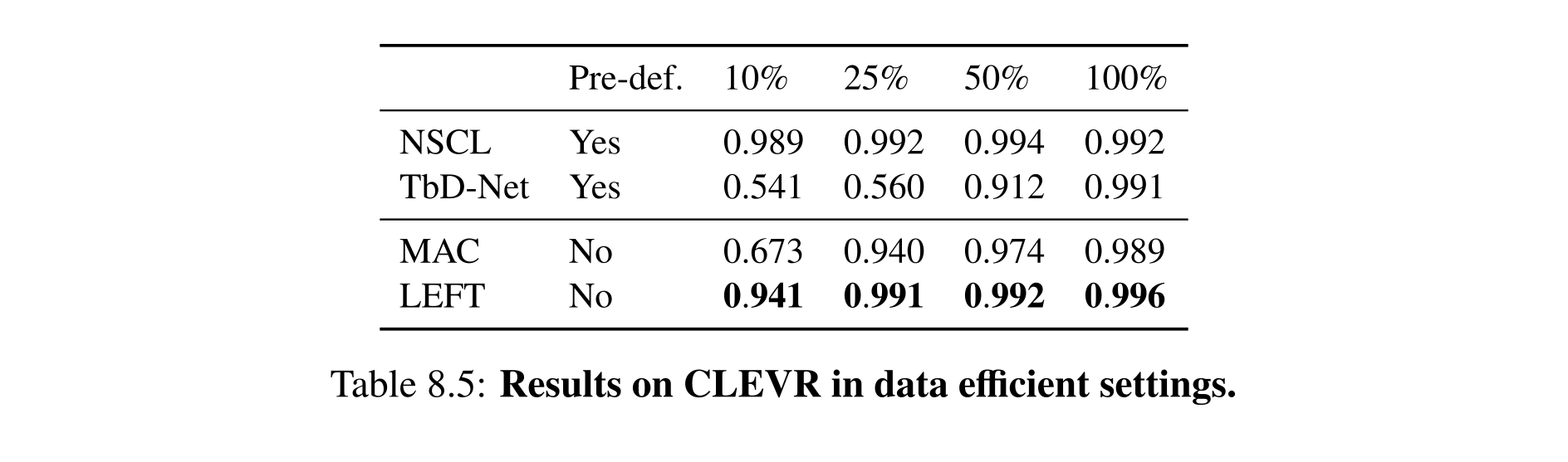
Table 8.5: Results on CLEVR in data efficient settings.
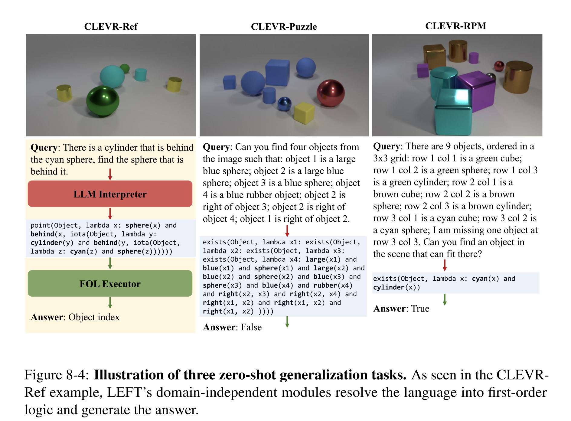
Figure 8-4: Illustration of three zero-shot generalization tasks. As seen in the CLEVR- Ref example, LEFT’s domain-independent modules resolve the language into first-order logic and generate the answer.
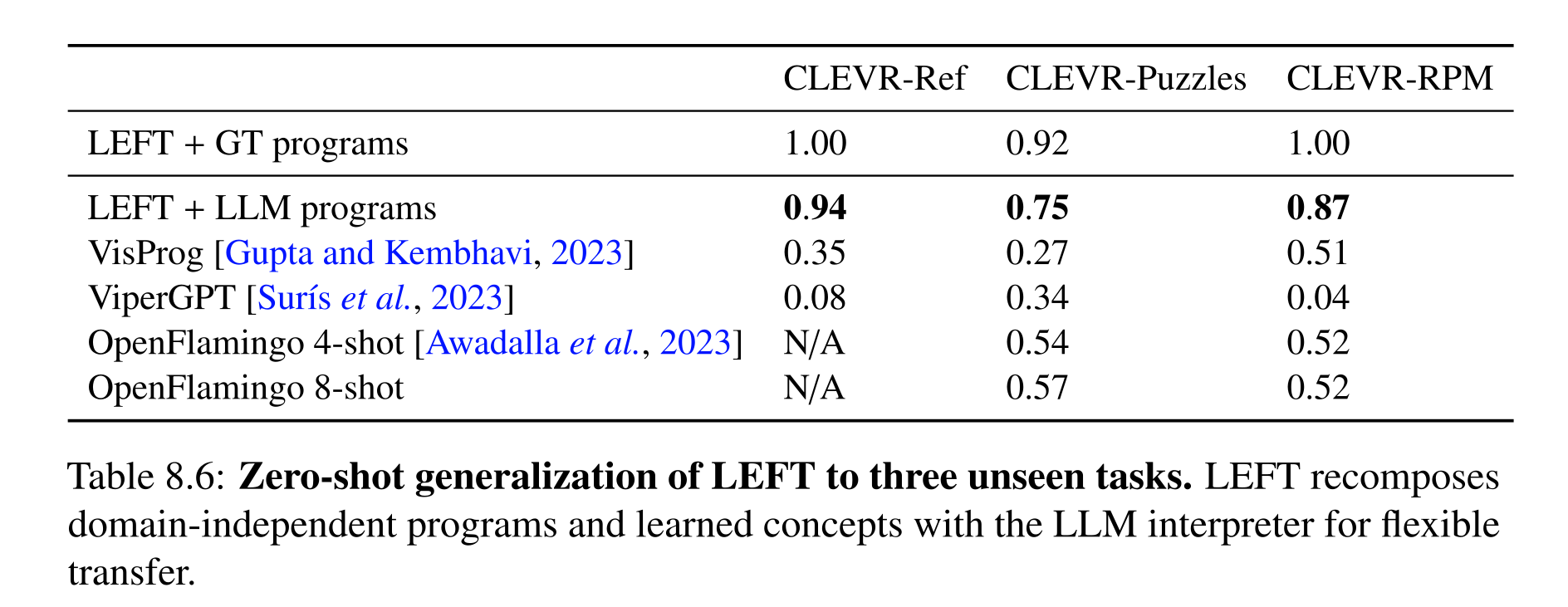
Table 8.6: Zero-shot generalization of LEFT to three unseen tasks. LEFT recomposes domain-independent programs and learned concepts with the LLM interpreter for flexible transfer.
Related Work
LEFT combines LLM program decomposition with the trainability of neuro-symbolic models. Its contribution is a shared differentiable logic language whose learned predicates can be grounded in several modalities, whereas the compared API-based systems depend on fixed pretrained operations and earlier neuro-symbolic systems define domain-specific program languages. These are comparisons to the evaluated systems, not a guarantee that all other architectures lack such capabilities.
Discussion
The experiments support modular grounding plus reusable logic as a route to efficient learning and reasoning transfer. LEFT does not model feedback between language interpretation and perception, speaker intent, or pragmatic ambiguity. Its independent concept modules also do not automatically share meanings across synonymous expressions; perception-informed interpretation and pragmatic learning remain future directions.
Visual Concept Lexicon
Grammar-Based Grounded Lexicon Learning (G2L2) jointly learns a word’s syntactic type, executable meaning, and associated perceptual concepts from grounded examples. A compact combinatory grammar composes these lexical entries into sentence programs. Based on Mao et al. (2021), the chapter reverses the earlier perspective: visual evidence helps acquire a language lexicon rather than merely grounding concepts supplied by a parser.
Introduction
The lexicalist hypothesis places most linguistic knowledge in richly structured word entries and uses a small set of composition rules. For example, “shiny” can learn a right-taking object-set modifier whose program filters by a grounded concept. Learning is difficult because candidate entries combine exponentially; G2L2 addresses this with joint chart parsing and local expected execution. Its strongest demonstrations concern recombining known constituents, under an assumption of context-independent word meanings.
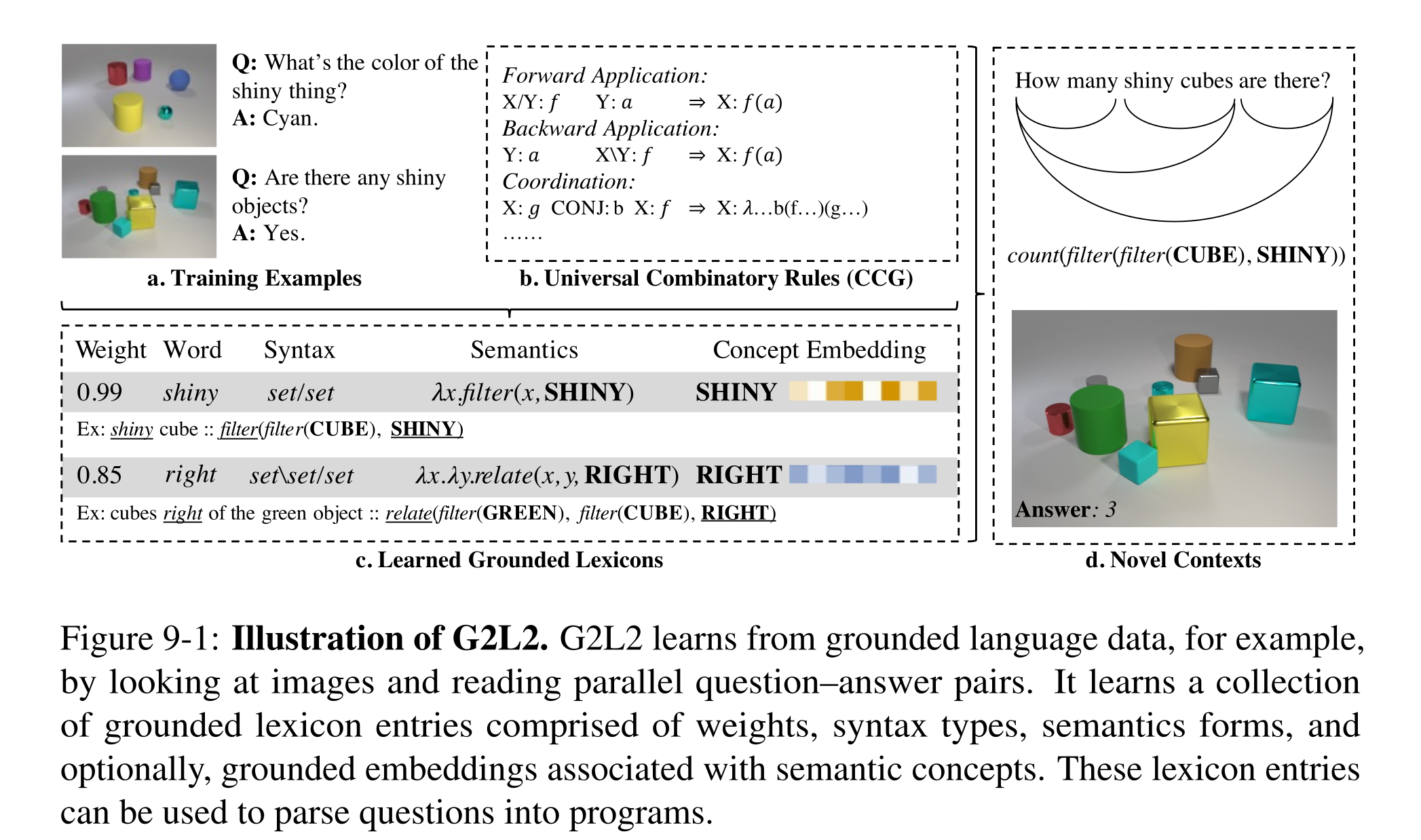
Figure 9-1: Illustration of G2L2. G2L2 learns from grounded language data, for example, by looking at images and reading parallel question–answer pairs. It learns a collection of grounded lexicon entries comprised of weights, syntax types, semantics forms, and optionally, grounded embeddings associated with semantic concepts. These lexicon entries can be used to parse questions into programs.
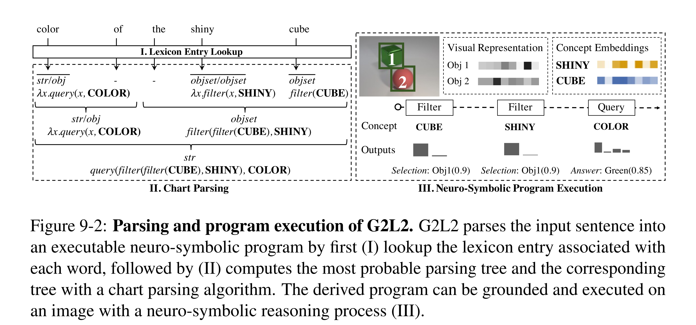
Figure 9-2: Parsing and program execution of G2L2. G2L2 parses the input sentence into an executable neuro-symbolic program by first (I) lookup the lexicon entry associated with each word, followed by (II) computes the most probable parsing tree and the corresponding tree with a chart parsing algorithm. The derived program can be grounded and executed on an image with a neuro-symbolic reasoning process (III).
Grammar-Based Grounded Lexicon Learning
Each token supplies candidate lexical entries; chart parsing combines their syntactic types and semantic programs; a differentiable executor grounds the resulting question program in the image. Answer supervision updates lexical weights and concept representations. The architecture does not require annotated word meanings or training question programs, but it does require manually specified domain operations and a constrained candidate lexicon space.
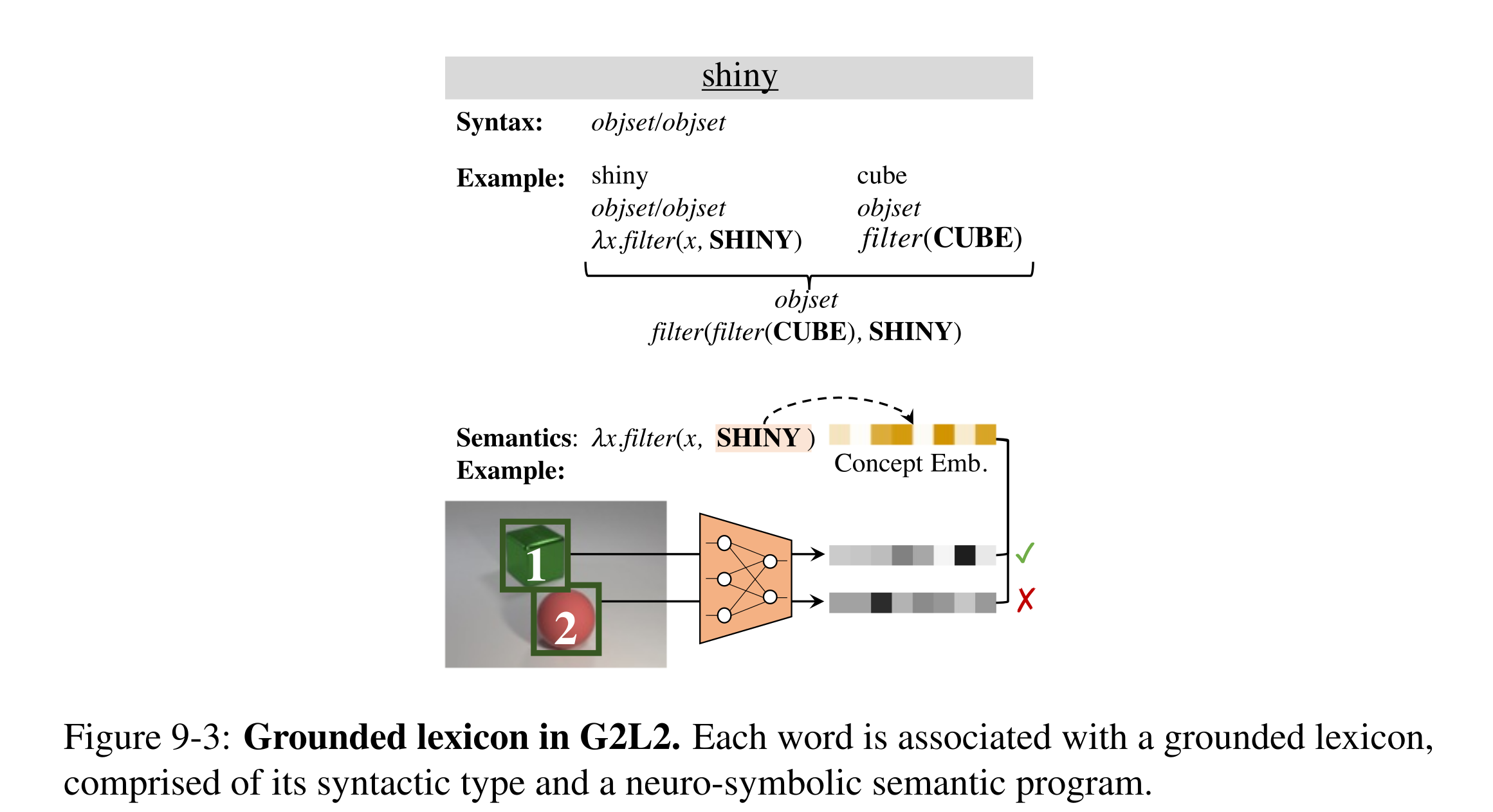
Figure 9-3: Grounded lexicon in G2L2. Each word is associated with a grounded lexicon, comprised of its syntactic type and a neuro-symbolic semantic program.
Grounded Lexicon
A lexical entry pairs a syntactic category with a typed semantic program. Forward and backward slashes specify which side supplies an argument, allowing word order and meaning composition to be learned together. Candidate programs and argument orderings are enumerated under arity/depth bounds; concept-bearing templates create word-specific embeddings. Although multiple candidates are considered during learning, the experiments assume one context-independent lexical entry per word type and exclude forms that violate this assumption.
Program Execution
Grounded programs operate on soft object sets and learned concept embeddings. Filtering multiplies the input set membership by the concept’s membership score; other modules compose the resulting tensors into an answer. This chapter uses product-based intersection rather than NS-CL’s minimum-based intersection, a deliberate change that makes more operations compatible with expected execution.
Joint Chart Parsing and Expected Execution (CKY-E2)
CKY-E2 builds spans in increasing length and merges candidate programs whose differing, fully bound subtrees can be executed to a common type. Their results are replaced by a weighted expectation, reducing repeated composition. Exactness requires each later operation to commute with expectation, with independence where multiplication is used; nonlinear quantifiers need approximation. The stated polynomial complexity assumes bounded arity and a bounded family of residual program layouts. Appendix I.1 uses log-sum-exp for merged log weights, unlike the main algorithm’s printed addition of log weights.
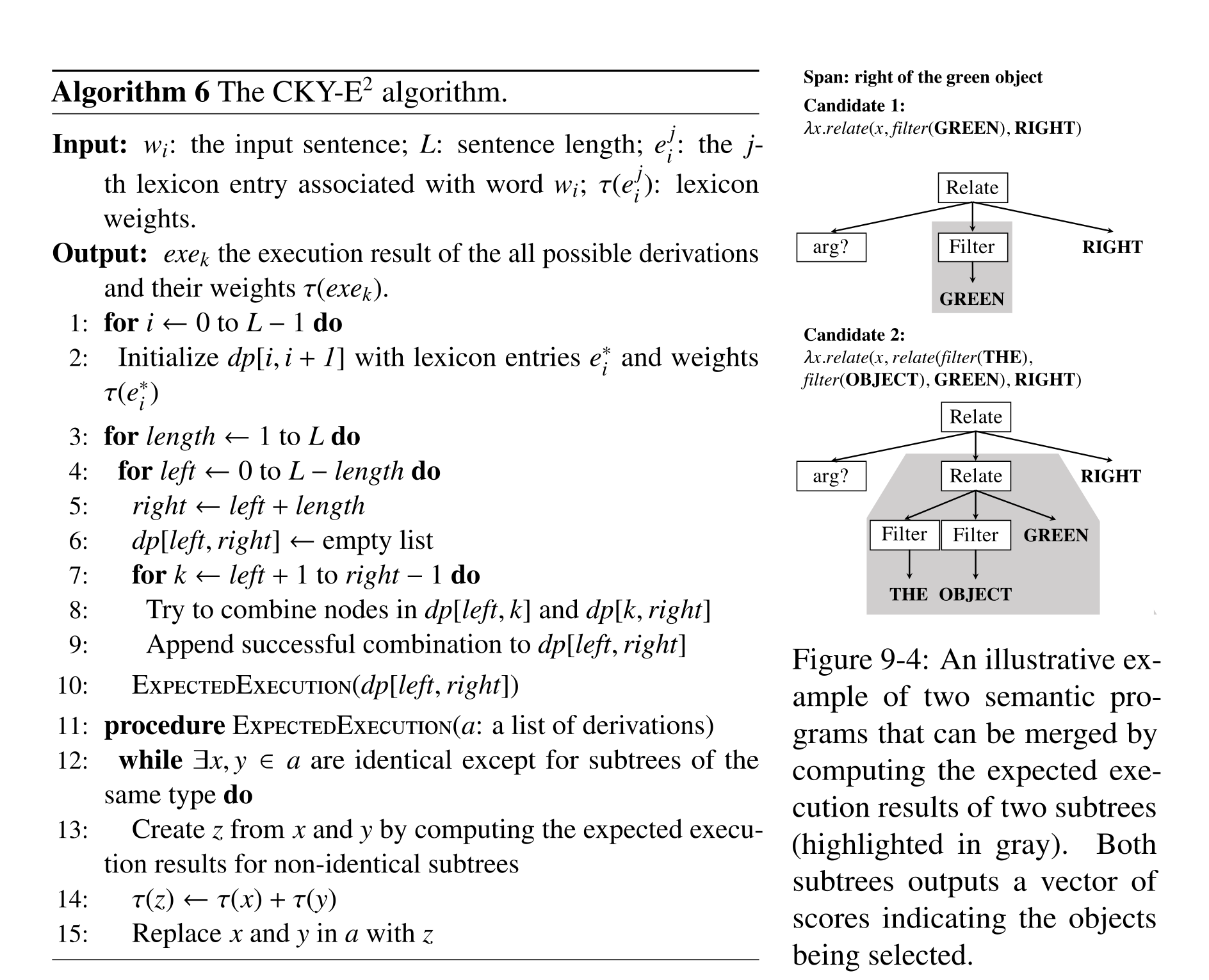
Figure 9-4: An illustrative ex- ample of two semantic pro- grams that can be merged by computing the expected exe- cution results of two subtrees (highlighted in gray). Both subtrees outputs a vector of scores indicating the objects being selected.
Equations


Learning
Lexical weights define a context-free distribution over derivations, and grounding parameters determine their executed answers. The stated objective averages the supervised answer loss over derivations and is optimized by gradients. Expected execution compresses intermediate results, but exact preservation of their expectation does not by itself imply exact preservation of an arbitrary nonlinear loss; the appendix’s example illustrates the former property.
Equation

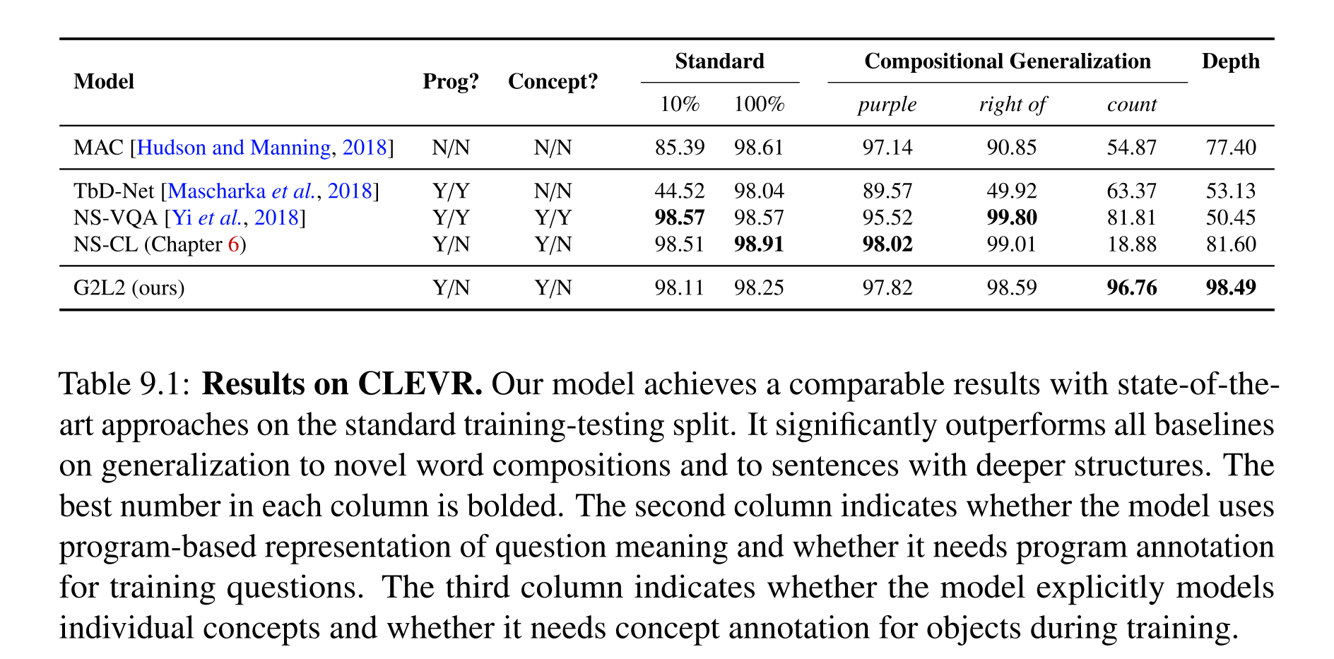
Table 9.1: Results on CLEVR. Our model achieves a comparable results with state-of-the- art approaches on the standard training-testing split. It significantly outperforms all baselines on generalization to novel word compositions and to sentences with deeper structures. The best number in each column is bolded. The second column indicates whether the model uses program-based representation of question meaning and whether it needs program annotation for training questions. The third column indicates whether the model explicitly models individual concepts and whether it needs concept annotation for objects during training.
Experiment
Experiments evaluate grounded visual reasoning on a filtered CLEVR language and instruction-to-action translation on SCAN. They separately test ordinary held-out examples, fewer training examples, restricted uses of selected words, and deeper or longer compositions. The benchmark languages match the framework’s constrained, largely unambiguous lexicon assumptions.
Visual Reasoning
CLEVR training uses a sentence-length curriculum on regenerated questions from 208 of the original 425 templates. G2L2 scores 98.11% with 10% data and 98.25% with all data. Its clearest advantages are held-out counting compositions (96.76%) and transfer from zero/one-hop to two-hop questions (98.49%). It is not best on every compositional split: Table 9.1 gives higher purple and right-of scores to other neuro-symbolic models. The results concern the filtered language, which excludes coreference, same-attribute questions, and numerical comparisons.
Language-driven Navigation
SCAN programs create, concatenate, and repeat action strings; candidate enumeration produces 178 lexical entries per word. G2L2 achieves exact-match accuracy of 1.00 on the reported simple, jump, around-right, and output-length splits, but these are selected successful runs. Across 100 training attempts, 74% reached perfect training accuracy; failed runs averaged 0.94, and training was restarted until successful. Ambiguous connective types for “and” and “after” explain common local optima. Thus perfect generalization is conditional on successful lexicon induction, not guaranteed for every initialization.
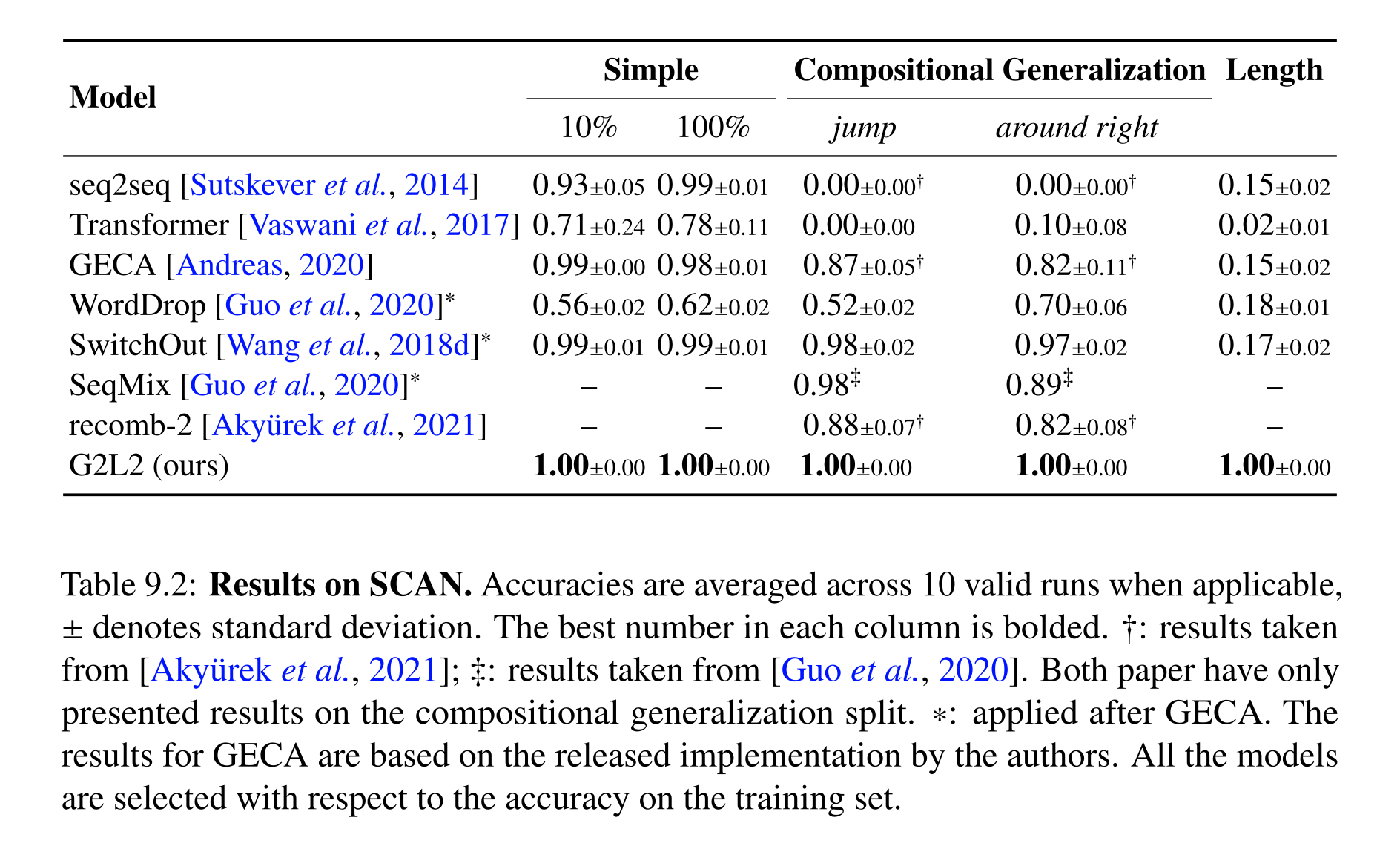
Table 9.2: Results on SCAN. Accuracies are averaged across 10 valid runs when applicable, ± denotes standard deviation. The best number in each column is bolded. †: results taken from [Aky¨urek et al., 2021]; ‡: results taken from [Guo et al., 2020]. Both paper have only presented results on the compositional generalization split. *: applied after GECA. The results for GECA are based on the released implementation by the authors. All the models are selected with respect to the accuracy on the training set.
Related Work
G2L2 joins lexicalist grammar, grounded language learning, and neuro-symbolic execution. Unlike latent-tree methods that summarize spans only as scores or vectors, CKY-E2 compresses typed executable programs, including partially bound functions. The proposed contribution is joint induction of syntax, semantic forms, and grounding under a specified grammar and DSL, rather than discovery of unrestricted linguistic structure.
Discussion
The learned lexicon supports strong recombination when word meanings and composition rules remain context independent. Handling ambiguity, pragmatics, broader semantic programs, and learning new words from an existing lexicon remain open. The experiments support the usefulness of explicit constituent composition without establishing that the restricted candidate spaces cover ordinary language.
III Neuro-Symbolic Action Concepts
Part III develops action concepts at three scales: reusable manipulation skills, learned models for long-horizon planning, and a language combining procedural knowledge with declarative constraints. These chapters share structured representations, but their assumptions and evaluations differ.
Neuro-Symbolic Skills
The chapter combines three approaches to reusable skills: contact-mode mechanisms learned from one demonstration plus simulator exploration; MAGIC, which transfers a demonstrated contact through visual and geometric analogy; and KALM, which learns trajectories around automatically proposed and verified keypoints. These are complementary systems, rather than one jointly evaluated end-to-end pipeline.
Introduction
A useful manipulation strategy can be represented by a sequence of changes in contact, such as grasping a ladle, hooking a target, replacing the ladle and grasping the target. Abstracting that sequence reduces discrete planning choices, while specialized samplers focus the continuous search. MAGIC addresses unfamiliar object geometry; KALM extends the representation toward articulated operations and learned execution trajectories.
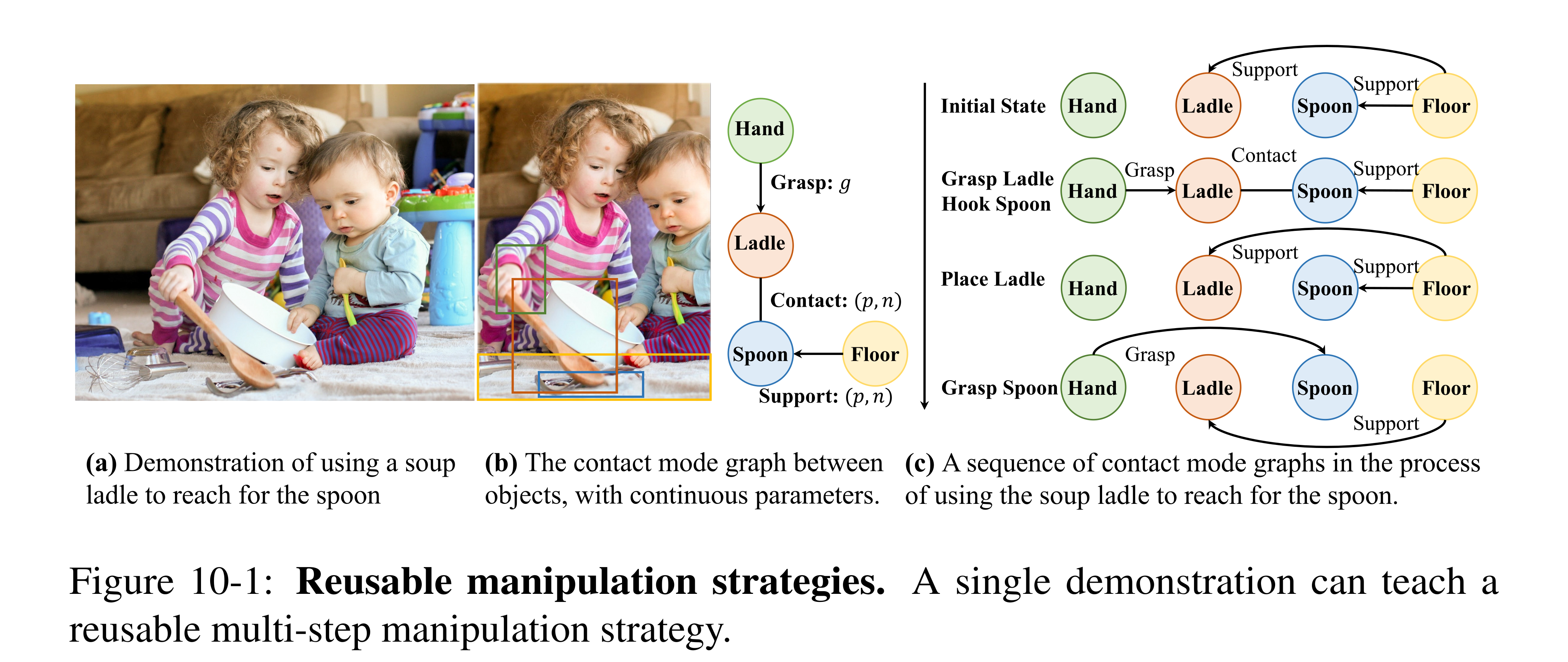
Figure 10-1: Reusable manipulation strategies. A single demonstration can teach a reusable multi-step manipulation strategy.
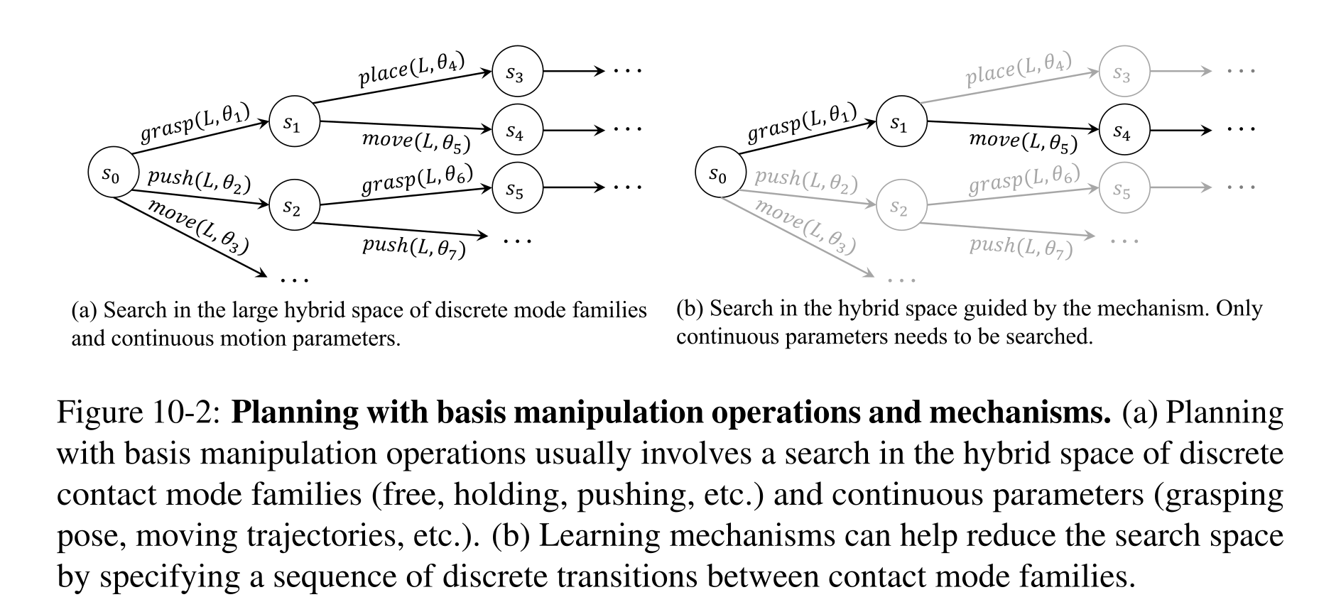
Figure 10-2: Planning with basis manipulation operations and mechanisms. (a) Planning with basis manipulation operations usually involves a search in the hybrid space of discrete contact mode families (free, holding, pushing, etc.) and continuous parameters (grasping pose, moving trajectories, etc.). (b) Learning mechanisms can help reduce the search space by specifying a sequence of discrete transitions between contact mode families.
Planning with Contacts and Mechanisms
Generic contact primitives are expressive but expensive to combine. Learned mechanisms act as macros in the same task-and-motion representation, shortening the effective search horizon without replacing geometric feasibility checks.
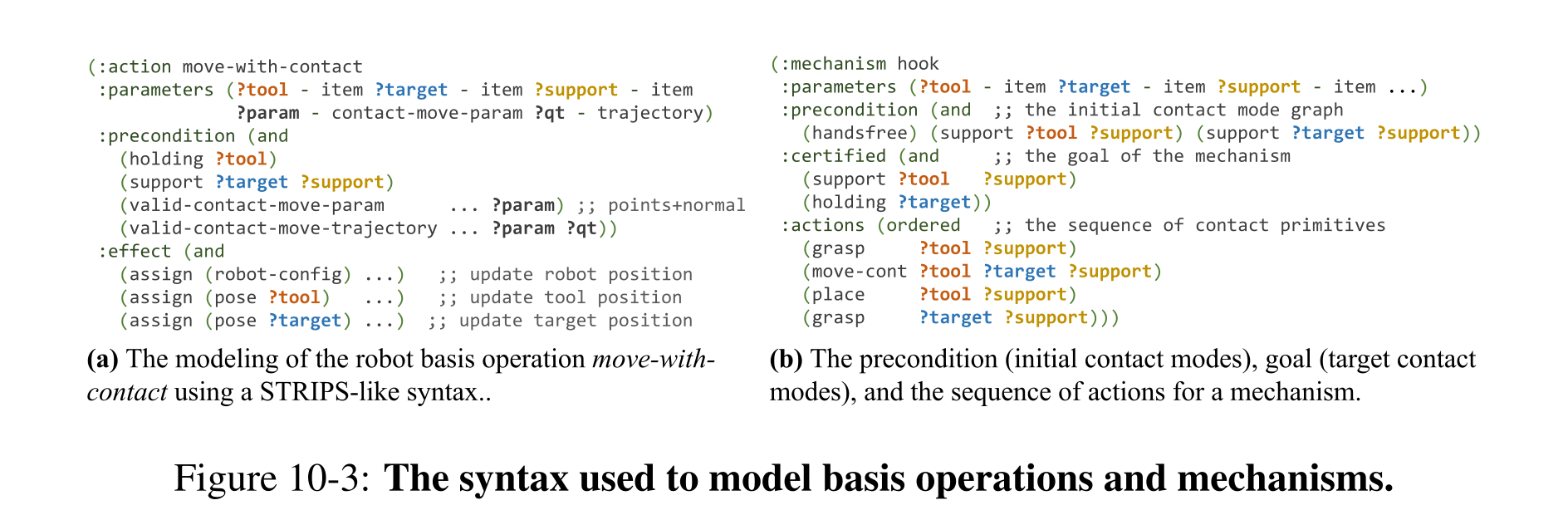
Figure 10-3: The syntax used to model basis operations and mechanisms.
Basic Domain Representation
The state contains a fixed set of objects, their shapes/poses and holding/support relations. An action schema specifies arguments, preconditions, effects and a continuous-parameter sampler. Six basis operations cover free movement, direct contact, grasping, placing, carrying and tool-mediated contact. This formulation assumes access to the object/state representation and an applicable transition model.
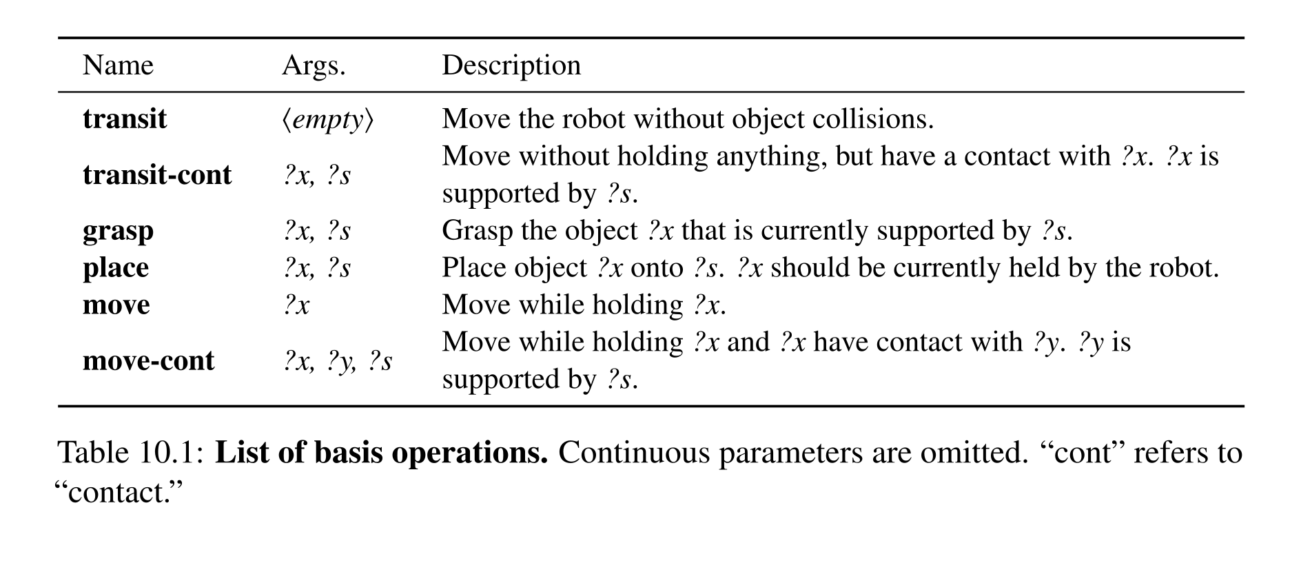
Table 10.1: List of basis operations. Continuous parameters are omitted. “cont” refers to “contact.”
Mechanisms
A mechanism packages object arguments, an initial contact graph, a certified goal, an ordered primitive sequence and a joint sampler. The hook macro grasps a tool, moves it against the target, replaces it and grasps the now-reachable target. Its symbolic structure generalizes across object identities, while sampling and simulation determine whether a particular instantiation works.
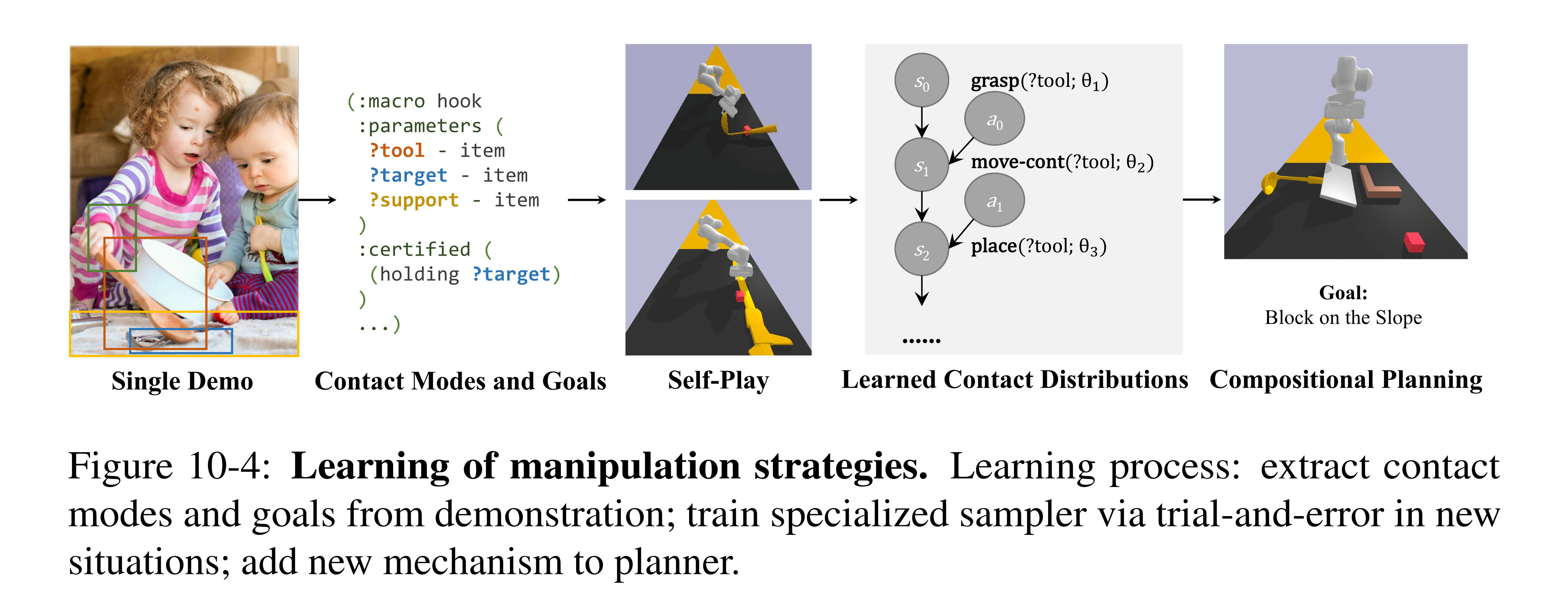
Figure 10-4: Learning of manipulation strategies. Learning process: extract contact modes and goals from demonstration; train specialized sampler via trial-and-error in new situations; add new mechanism to planner.
Planning with Basis Operators and Mechanisms
The planner searches discrete STRIPS plans with a fast-forward heuristic, samples grasps/contacts/trajectories, simulates their effects and backtracks when continuous choices fail. Mechanisms enter as additional operators, following the bilevel approach of PDDLStream. Simulation permits briefly dynamic transitions such as tipping or sliding between stable states; this is not unrestricted dynamic control.
Learning New Mechanisms
Learning requires a demonstrated action/contact sequence, a human-specified goal and a simulator that produces task-feasible initial configurations. The algorithm extracts a reusable operation sequence, explores its continuous parameters in new scenes, then learns scores that rank promising samples. “One demonstration” therefore does not mean learning without subsequent interaction data.
Extraction of Preconditions and Operation Sequence
Segment the demonstration when contact modes change; build graphs for the hand, directly/indirectly contacted objects and their supports. The initial graph supplies preconditions, and replacing concrete object names with variables lifts the sequence into a reusable schema. The desired certified goal is supplied by the human.
Sampler Learning
Self-play fixes the demonstrated discrete sequence but searches object bindings and continuous choices. Samples in the final successful plan are labeled positive, other tried samples negative; binary classifiers then rank batches from generic samplers. Later scores condition on earlier choices, giving a factorized joint proposal and allowing early backtracking. These search-derived labels are not a proof that every unused sample is intrinsically infeasible.
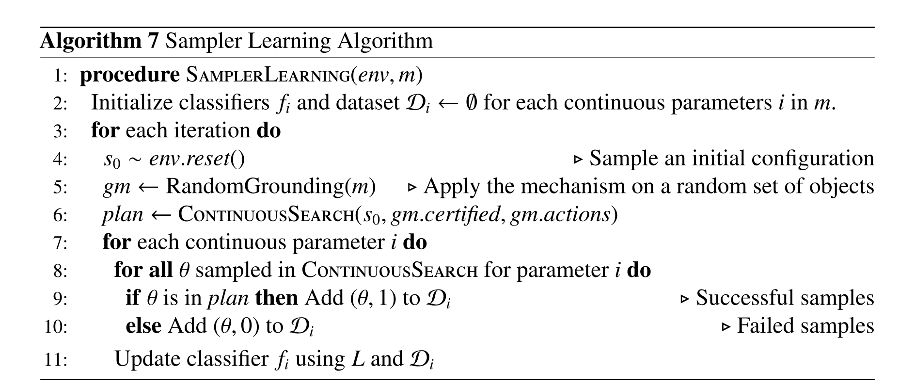
Implementation
Geometry-based samplers generate grasps, placements, object contacts and robot trajectories. Contact points/normals are aligned while excluding pushes toward the support surface. Learned scorers combine PointNet++ shape encodings with MLP encodings of poses and contacts; each is trained on 100 samples. The implementation scores contact motions by direction/distance but does not learn a classifier over complete arm paths.
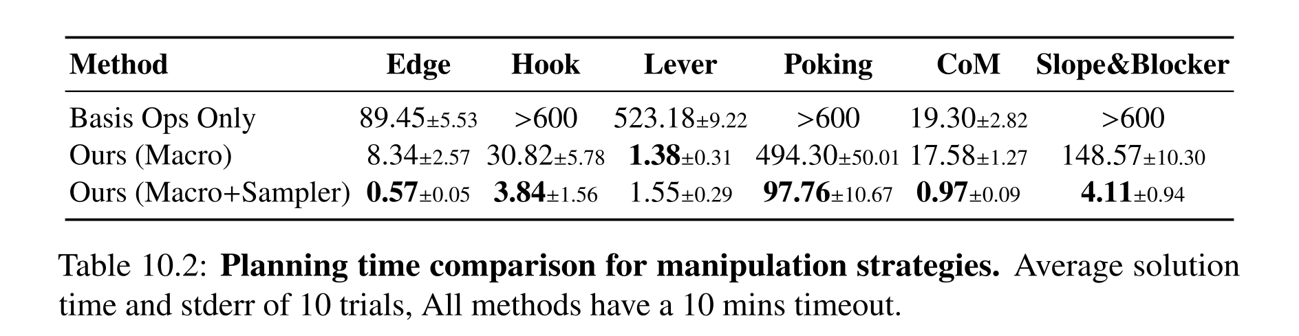
Table 10.2: Planning time comparison for manipulation strategies. Average solution time and stderr of 10 trials, All methods have a 10 mins timeout.
Experiments
PyBullet experiments evaluate six individual mechanisms and two new compositions. Training and test configurations are designed to admit the intended strategy; demonstrations are scripted. Appendix J gives sampler details and physical deployment.
Learning Mechanisms from Single Demonstrations
Across ten trials with a ten-minute timeout, macros plus learned samplers reduce mean search time sharply: hooking falls from timeout with primitives to 3.84 seconds, and slope/blocker from timeout to 4.11 seconds. Benefits vary: lever planning is already easy once its macro is known, whereas narrow collision-free poking motions still average 97.76 seconds. The table measures planning time, not robot execution duration or broad unrestricted-scene robustness.
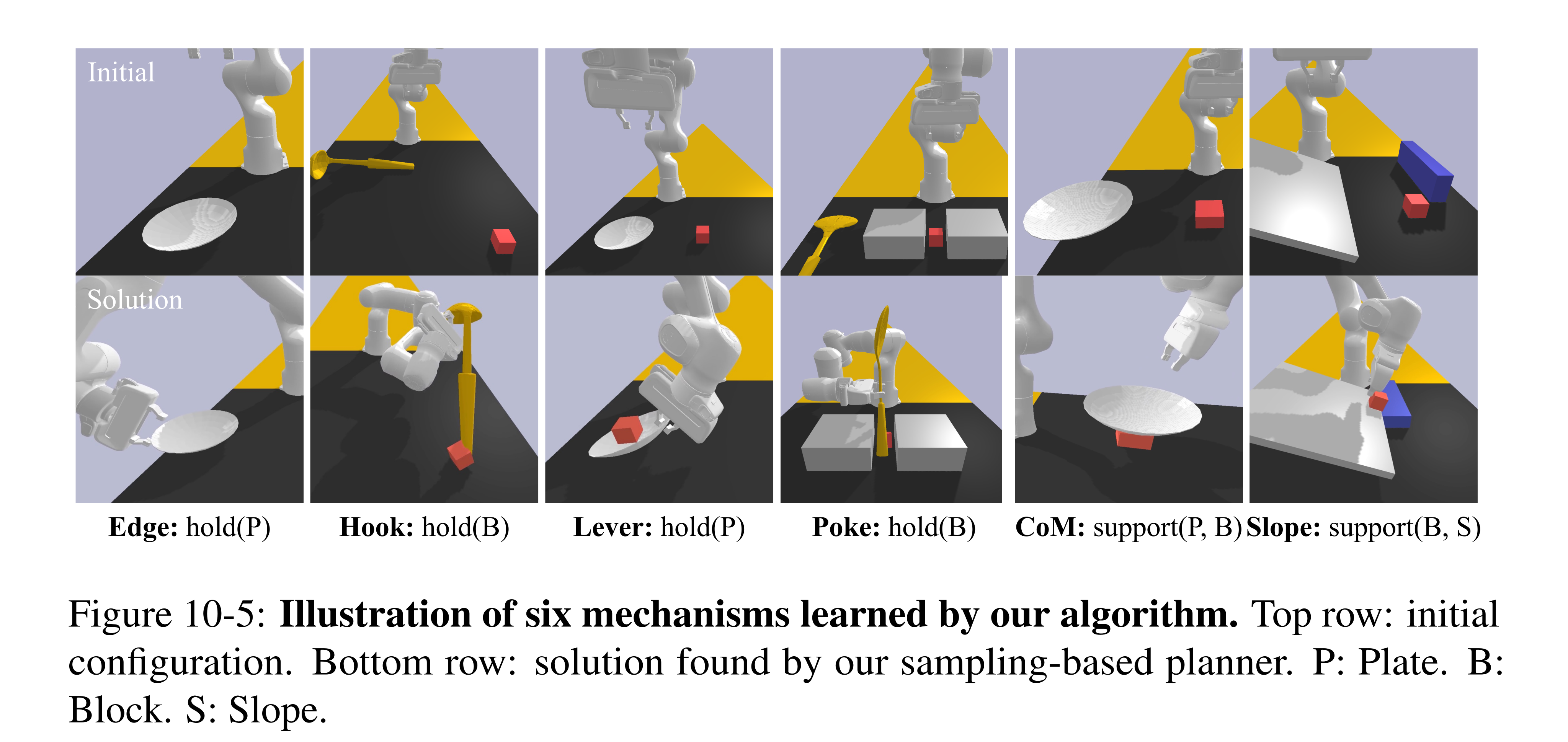
Figure 10-5: Illustration of six mechanisms learned by our algorithm. Top row: initial configuration. Bottom row: solution found by our sampling-based planner. P: Plate. B: Block. S: Slope.
Planning with Learned Mechanisms
Previously learned mechanisms are recombined without additional training to push/pick/use a caliper and to hook an object then stabilize it on a slope. With ten runs and ten-minute timeouts, macros plus samplers solve 100% and 90%; primitives solve neither, and macros alone solve 20% and 0%. Table 10.3 reports success rates despite the surrounding prose calling it planning time. Task placements are deliberately feasible.
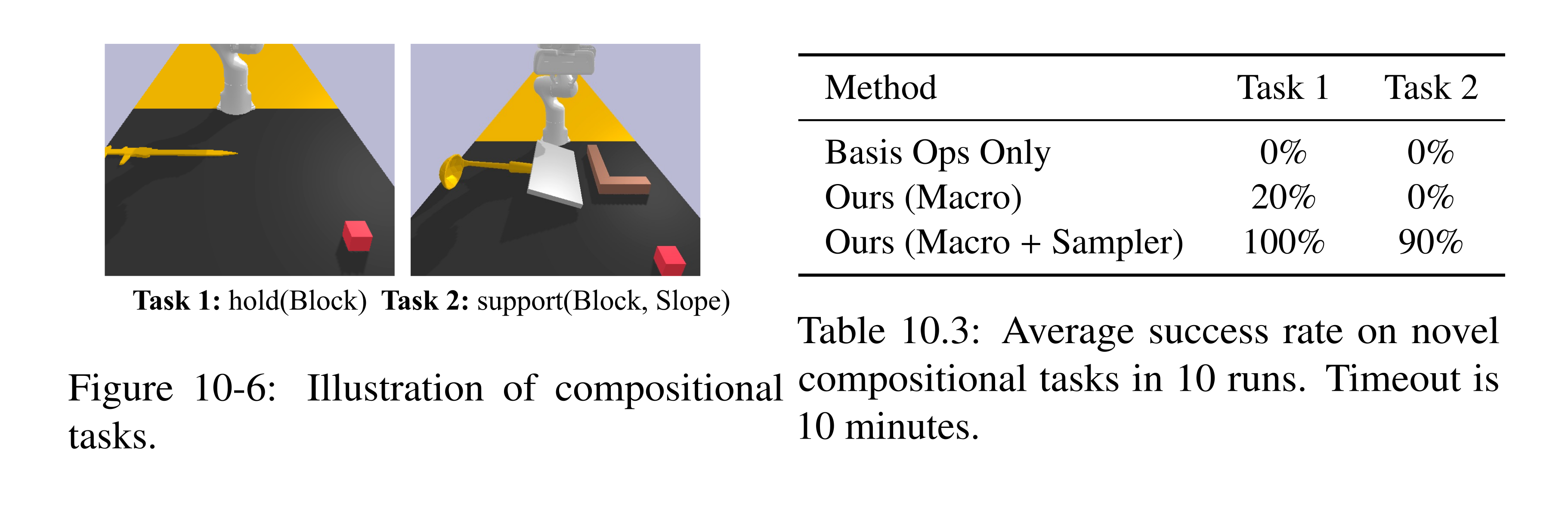
Figure 10-6: Illustration of compositional tasks.
Table 10.3: Average success rate on novel compositional tasks in 10 runs. Timeout is 10 minutes.
One-Shot Manipulation Strategy Learning
MAGIC transfers contact affordances through two stages: pretrained features propose globally analogous regions, then local curvature refines contact points and normals. The resulting correspondences guide retargeting, planning or tool selection, followed by simulator verification where available. The method reuses broad visual pretraining rather than learning a task-specific object representation from the single example.
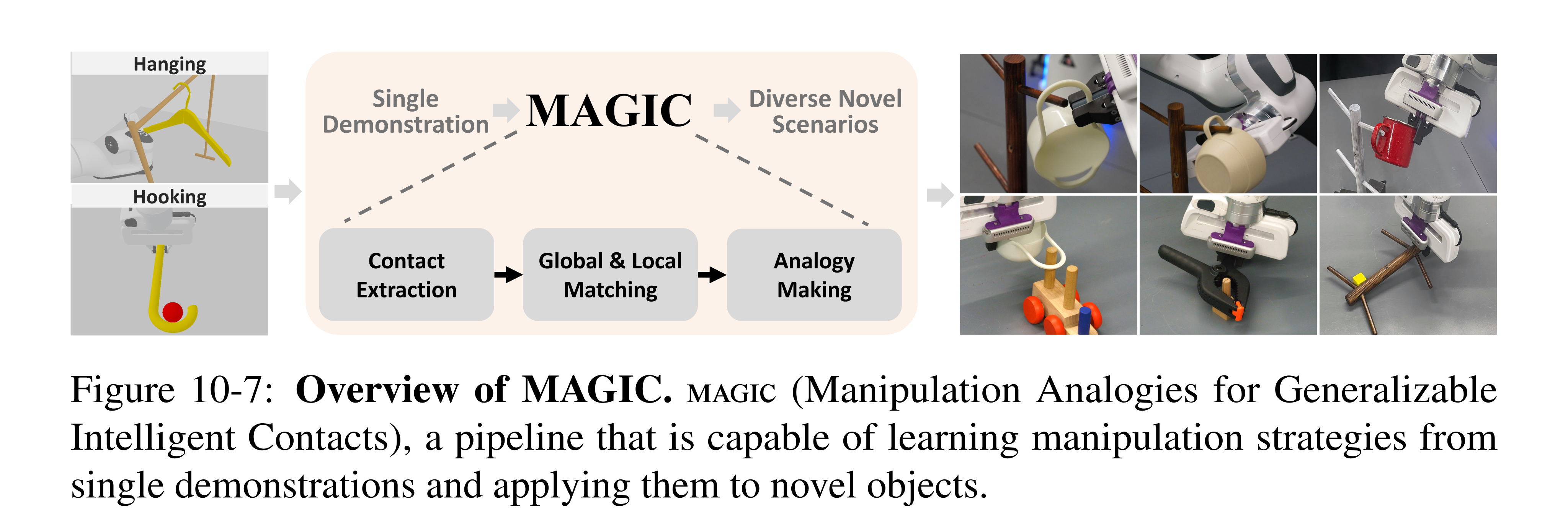
Figure 10-7: Overview of MAGIC. magic (Manipulation Analogies for Generalizable Intelligent Contacts), a pipeline that is capable of learning manipulation strategies from single demonstrations and applying them to novel objects.
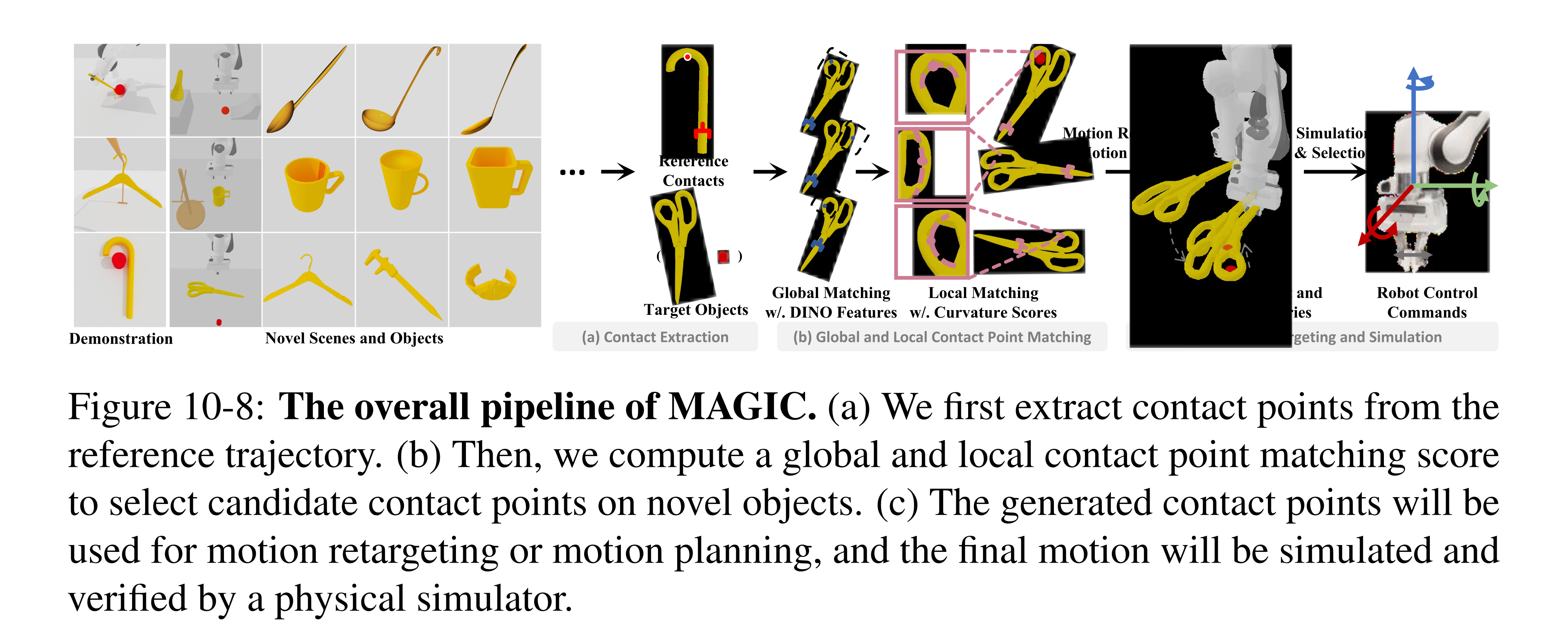
Figure 10-8: The overall pipeline of MAGIC. (a) We first extract contact points from the reference trajectory. (b) Then, we compute a global and local contact point matching score to select candidate contact points on novel objects. (c) The generated contact points will be used for motion retargeting or motion planning, and the final motion will be simulated and verified by a physical simulator.
Problem Definition
The evaluated setting assumes known reference/target objects, a specified strategy and a supplied canonical 2D view. One relevant contact waypoint and reduced-dimensional geometry determine an analogous rigid-body transform; real reference contacts are manually annotated. Main tasks use quasi-static simulation with reconstructed geometry and assumed physical properties. The proposed fallback for hard-to-simulate dynamics chooses the top match without that verification; multiple-contact generality is not established by these tests.
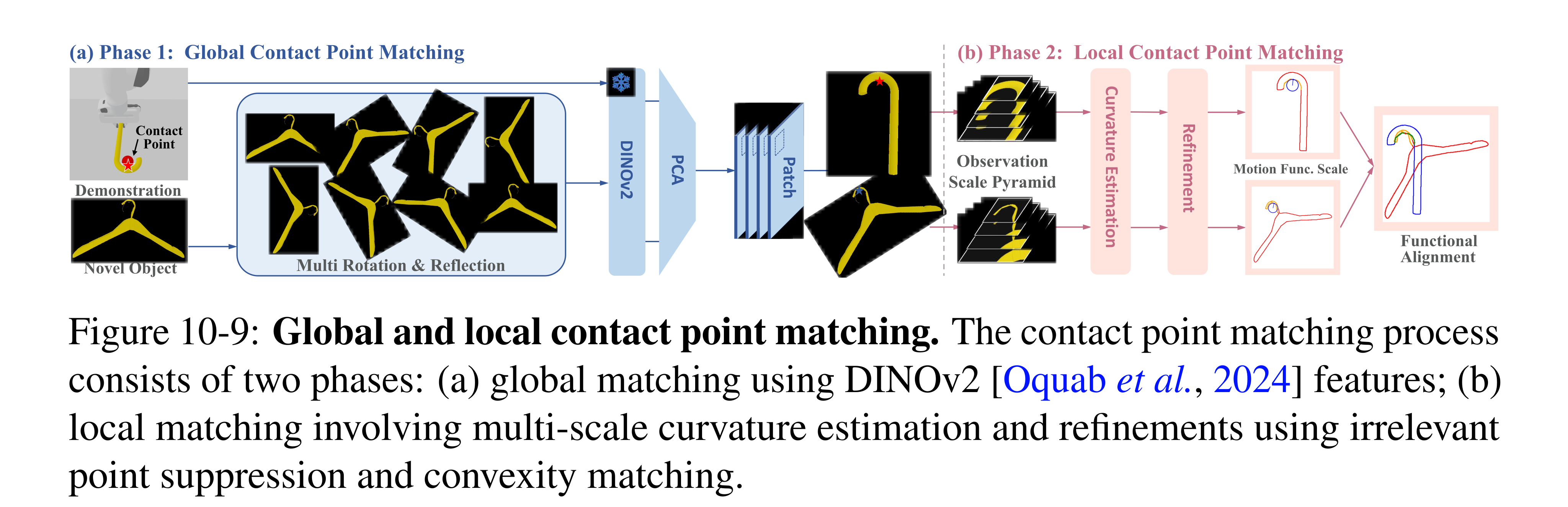
Figure 10-9: Global and local contact point matching. The contact point matching process consists of two phases: (a) global matching using DINOv2 [Oquab et al., 2024] features; (b) local matching involving multi-scale curvature estimation and refinements using irrelevant point suppression and convexity matching.
Equation

Global Contact Point Matching with Pretrained Features
DINOv2 features are extracted from the reference and 24 reflected/rotated target views, reduced jointly with PCA and compared over patches. The top three matches seed local refinement. This stage identifies plausible global regions, not precise contact geometry. DINOv2 supplies the pretrained visual representation.
Equation

Local Contact Point Matching with Curvature Estimation
Segmented edges are analyzed at several scales. A local principal-axis frame and quadratic fit estimate curvature; a scale/radius heuristic chooses the useful observation scale. Ray-based suppression removes nearby points belonging to a different edge, and local search matches convexity before re-estimation. The contact criterion compares curvature-radius ratios across the two interacting object pairs. The printed absolute ratio difference is a mismatch quantity, although the earlier combined expression is described as a score to maximize; its sign convention should not be silently treated as unambiguous.
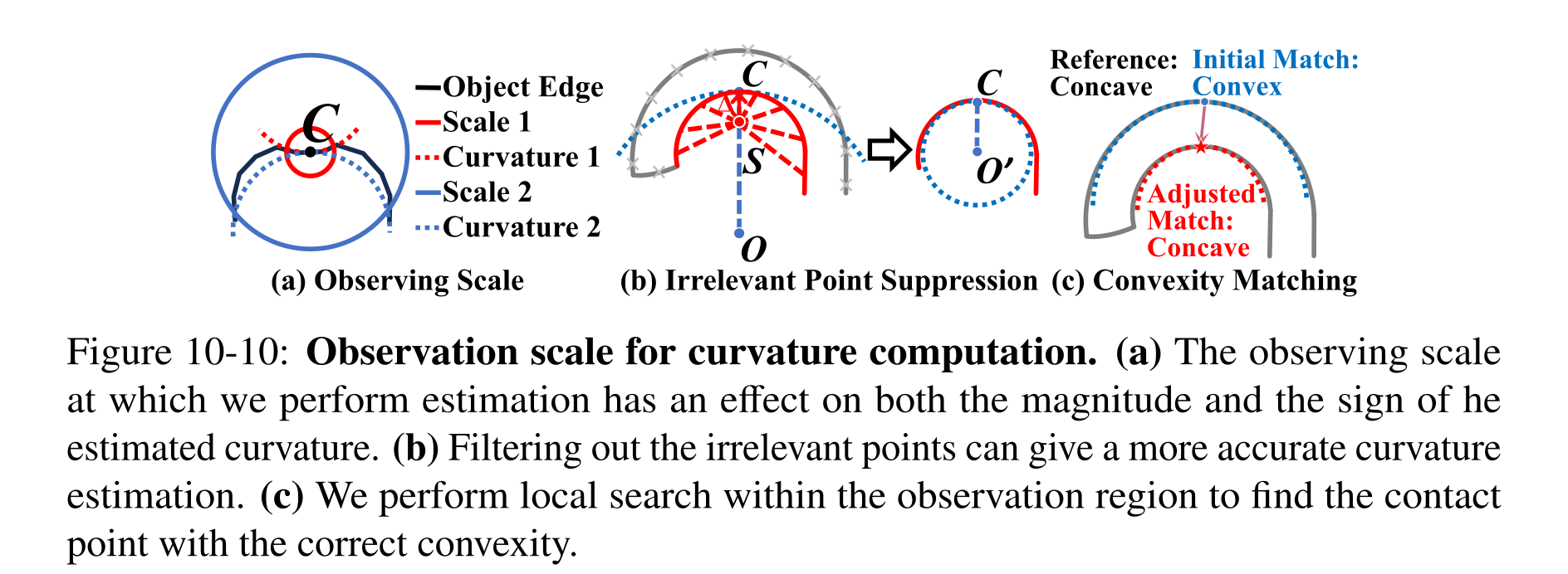
Figure 10-10: Observation scale for curvature computation. (a) The observing scale at which we perform estimation has an effect on both the magnitude and the sign of he estimated curvature. (b) Filtering out the irrelevant points can give a more accurate curvature estimation. (c) We perform local search within the observation region to find the contact point with the correct convexity.
Equations


Generating Object Motions by Making Contact Analogies
Matched contact points, normals and view directions define local frames for trajectory retargeting. Alternatively, the match supplies an end pose or force-direction waypoint for motion planning. Running the matcher over available tools enables selection by the contact score. Robot reachability and collisions still require separate checks.
Experiment Setup
SAPIEN tests cover scooping, hanging and hooking, with both a directly controlled floating tool and a harder robot-arm variant using antipodal grasps and RRT-Connect. Baselines use PCA/FPFH global alignment, DINO-only matching or sampled curvature matching; the latter is capped at 180 seconds. The floating-gripper condition excludes robot grasping/reachability and should not be reported as full robot success.
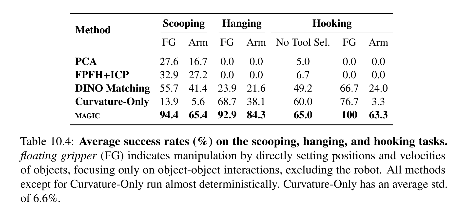
Table 10.4: Average success rates (%) on the scooping, hanging, and hooking tasks. floating gripper (FG) indicates manipulation by directly setting positions and velocities of objects, focusing only on object-object interactions, excluding the robot. All methods except for Curvature-Only run almost deterministically. Curvature-Only has an average std. of 6.6%.
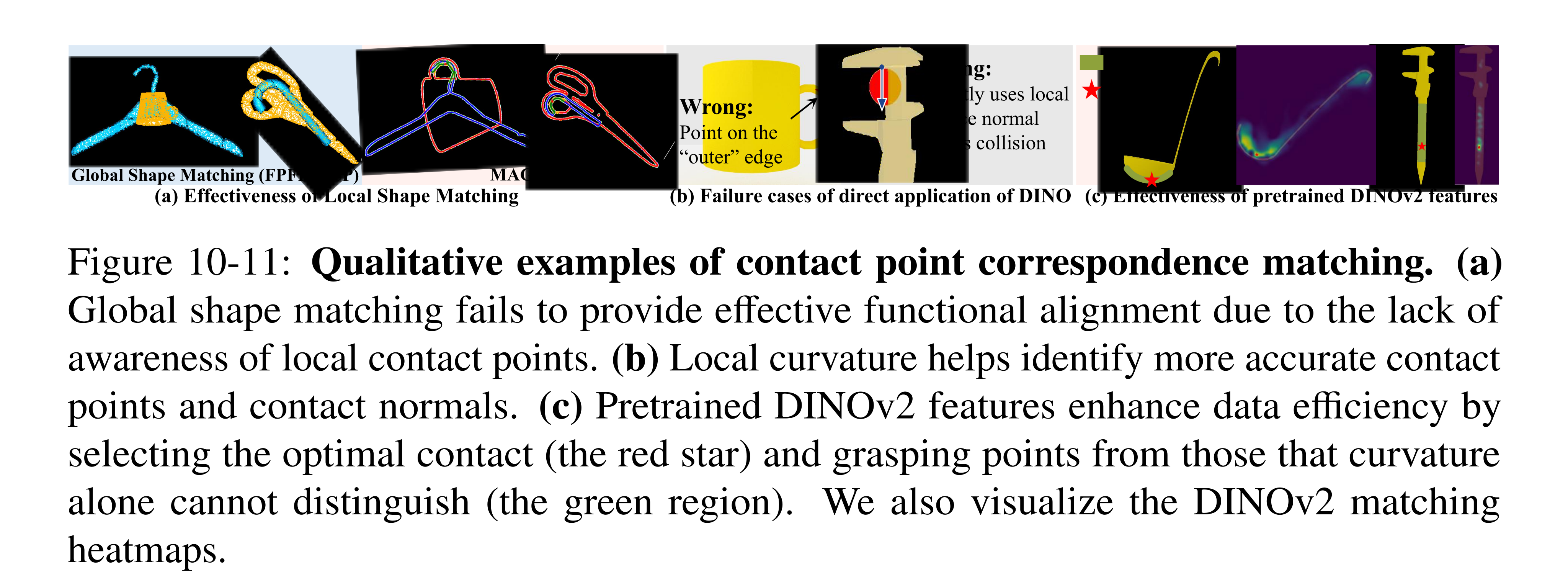
Figure 10-11: Qualitative examples of contact point correspondence matching. (a) Global shape matching fails to provide effective functional alignment due to the lack of awareness of local contact points. (b) Local curvature helps identify more accurate contact points and contact normals. (c) Pretrained DINOv2 features enhance data efficiency by selecting the optimal contact (the red star) and grasping points from those that curvature alone cannot distinguish (the green region). We also visualize the DINOv2 matching heatmaps.
Simulation Experiments
MAGIC reaches 94.4%, 92.9% and 100% in floating-gripper scooping, hanging and hooking, versus 65.4%, 84.3% and 63.3% with the arm. Tests span six spoons/three scoop objects, 134 mugs and four hook tools/five objects. Hanging transfer remains strong within and across categories. DINOv2 plus curvature averages 34 seconds in the feature comparison; alternative features are slower and mostly less accurate.
Ablations show that local refinement and simulator verification matter: without verification, the three floating-gripper scores fall to 77.8%, 71.6% and 50%. Removing feature PCA/patch aggregation slightly improves hanging (93.3% versus 92.9%) while harming the other tasks, so no component wins uniformly. A separate KETO-task comparison gives MAGIC 64.4% mean hammering and 76.3% pushing, against 56.4% and 71.7%; it uses a different benchmark and training regime, not the principal three-task comparison.
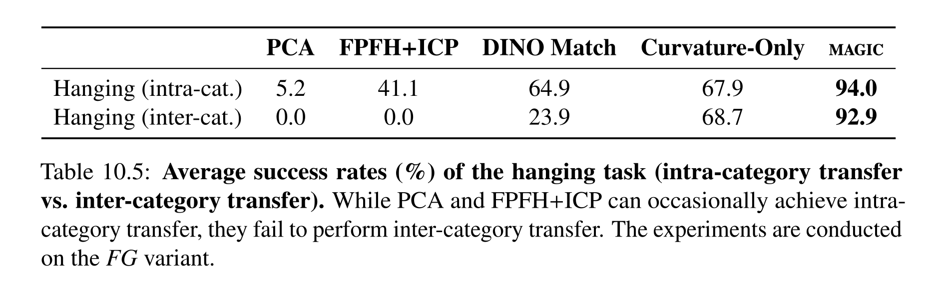
Table 10.5: Average success rates (%) of the hanging task (intra-category transfer vs. inter-category transfer). While PCA and FPFH+ICP can occasionally achieve intra- category transfer, they fail to perform inter-category transfer. The experiments are conducted on the FG variant.
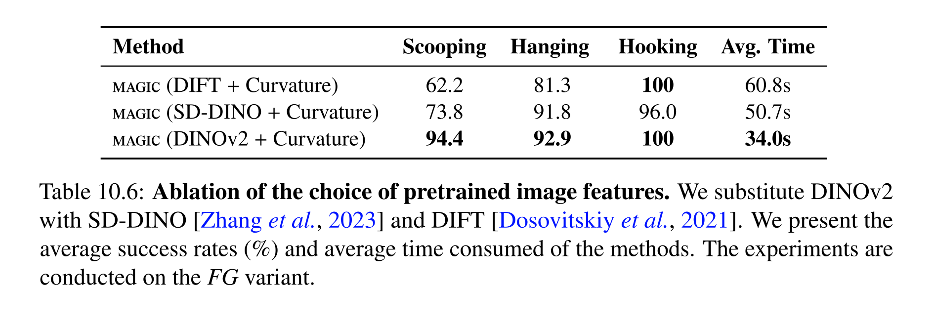
Table 10.6: Ablation of the choice of pretrained image features. We substitute DINOv2 with SD-DINO [Zhang et al., 2023] and DIFT [Dosovitskiy et al., 2021]. We present the average success rates (%) and average time consumed of the methods. The experiments are conducted on the FG variant.
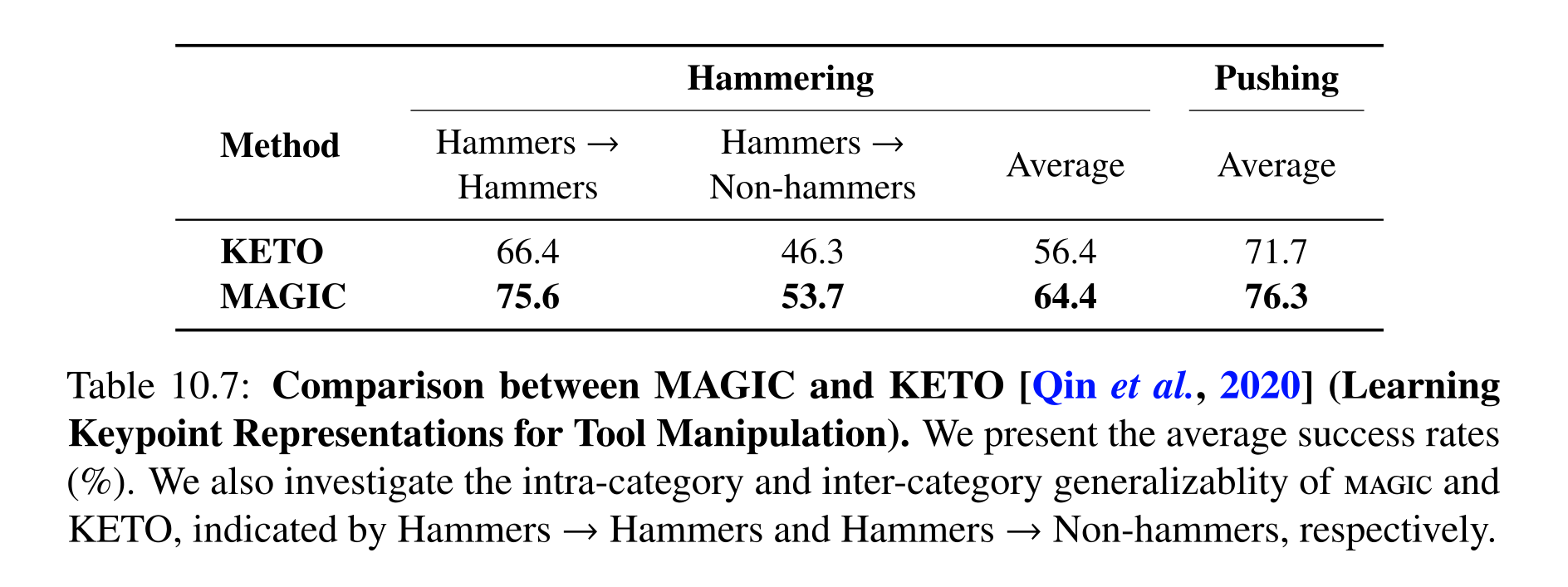
Table 10.7: Comparison between MAGIC and KETO [Qin et al., 2020] (Learning Keypoint Representations for Tool Manipulation). We present the average success rates (%). We also investigate the intra-category and inter-category generalizablity of magic and KETO, indicated by Hammers →Hammers and Hammers →Non-hammers, respectively.
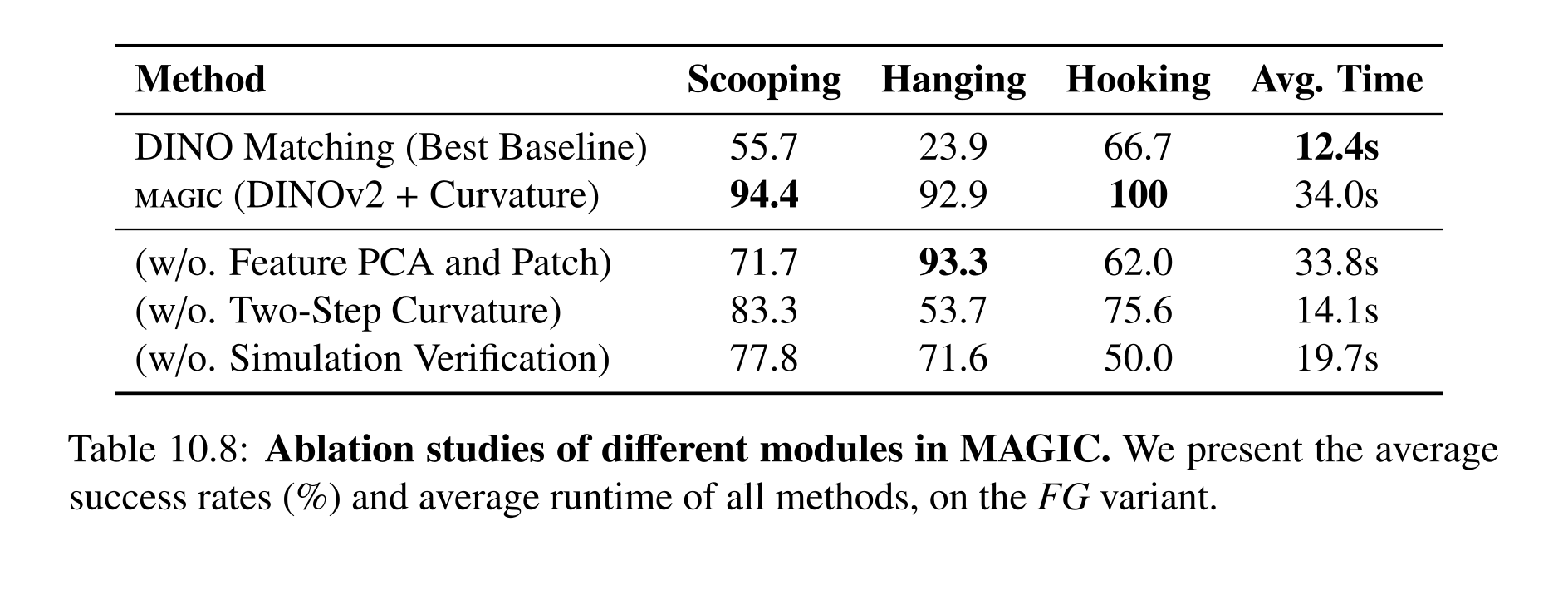
Table 10.8: Ablation studies of different modules in MAGIC. We present the average success rates (%) and average runtime of all methods, on the FG variant.
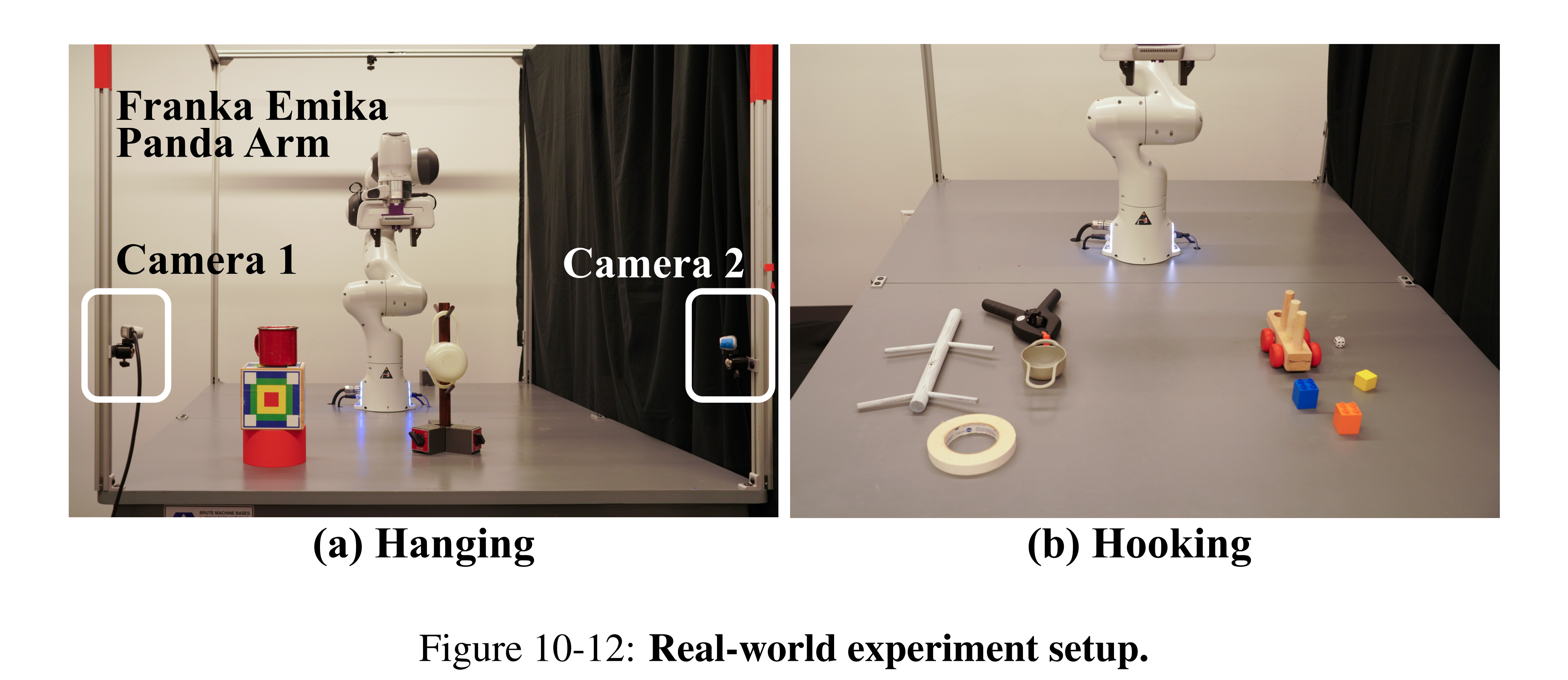
Figure 10-12: Real-world experiment setup.
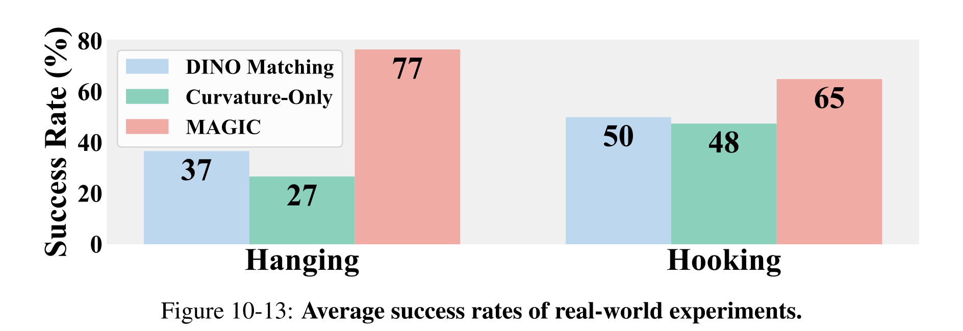
Figure 10-13: Average success rates of real-world experiments.
Real-World Experiments
A calibrated two-camera Franka setup reconstructs partial meshes using segmentation, outlier filtering, table-plane completion and Alpha Shapes, then plans/verifies in SAPIEN. Ten trials per object cover three cups and four tools. Reported success is about 77% for hanging and 65% for hooking, higher than DINO-only and curvature-only baselines. This supports the tested objects and reconstruction assumptions; it does not remove the dependence on canonical views, contact annotation or physical-model fidelity.
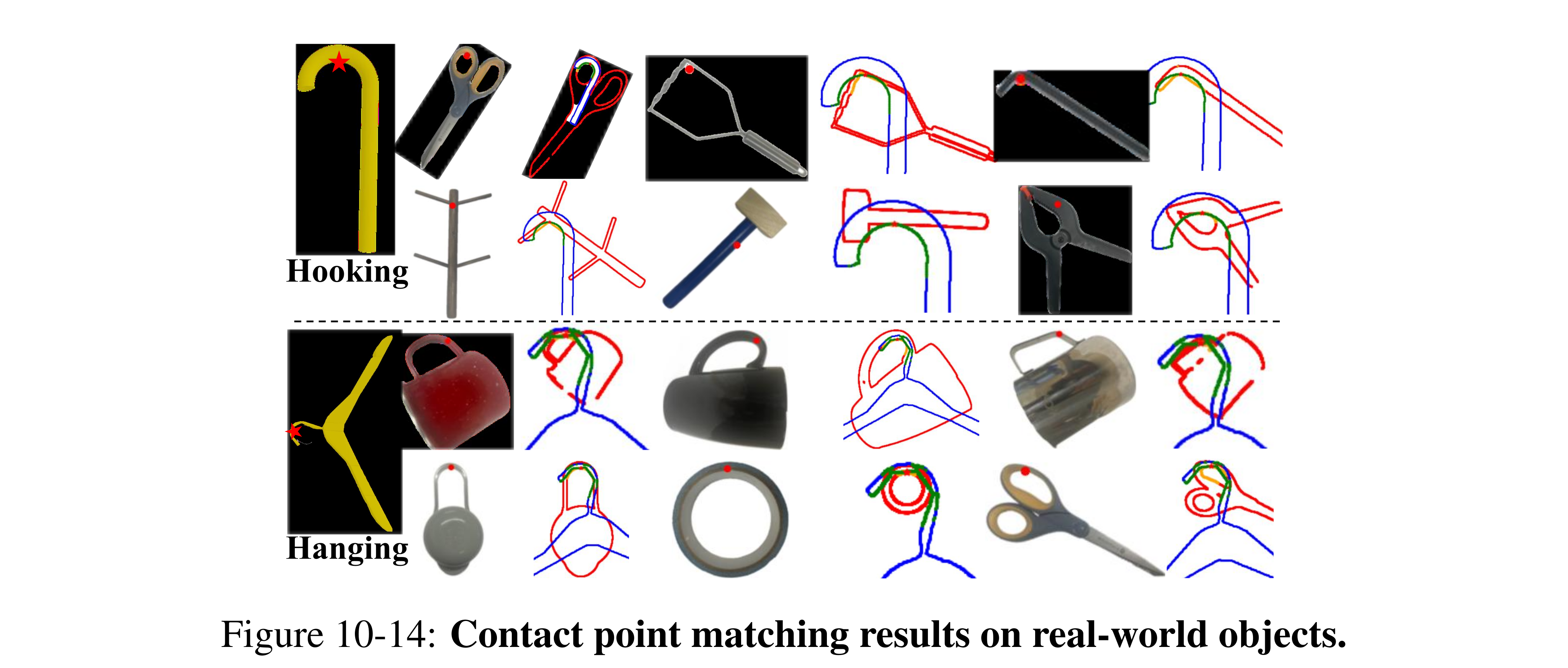
Figure 10-14: Contact point matching results on real-world objects.
Keypoint-Based Manipulation Strategy Learning
KALM proposes task-relevant object parts with a VLM, verifies keypoint correspondences across a small demonstration set, and learns keypoint-conditioned execution trajectories. The abstraction is intended to discard background variation while retaining task geometry. It uses a demonstration video, task description and roughly five to ten calibrated robot demonstrations, without additional manual keypoint labels in its real-world pipeline.
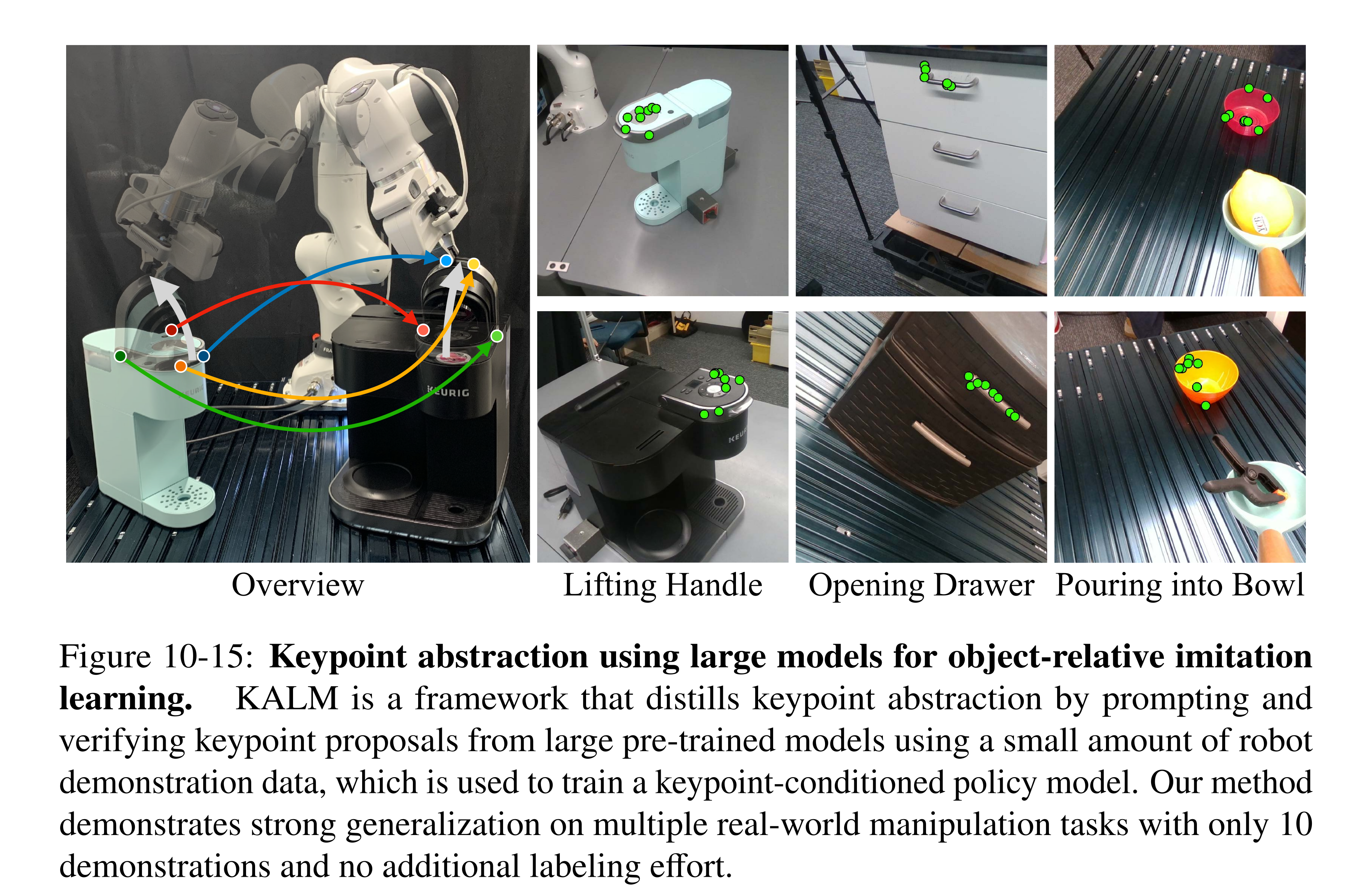
Figure 10-15: Keypoint abstraction using large models for object-relative imitation learning. KALM is a framework that distills keypoint abstraction by prompting and verifying keypoint proposals from large pre-trained models using a small amount of robot demonstration data, which is used to train a keypoint-conditioned policy model. Our method demonstrates strong generalization on multiple real-world manipulation tasks with only 10 demonstrations and no additional labeling effort.
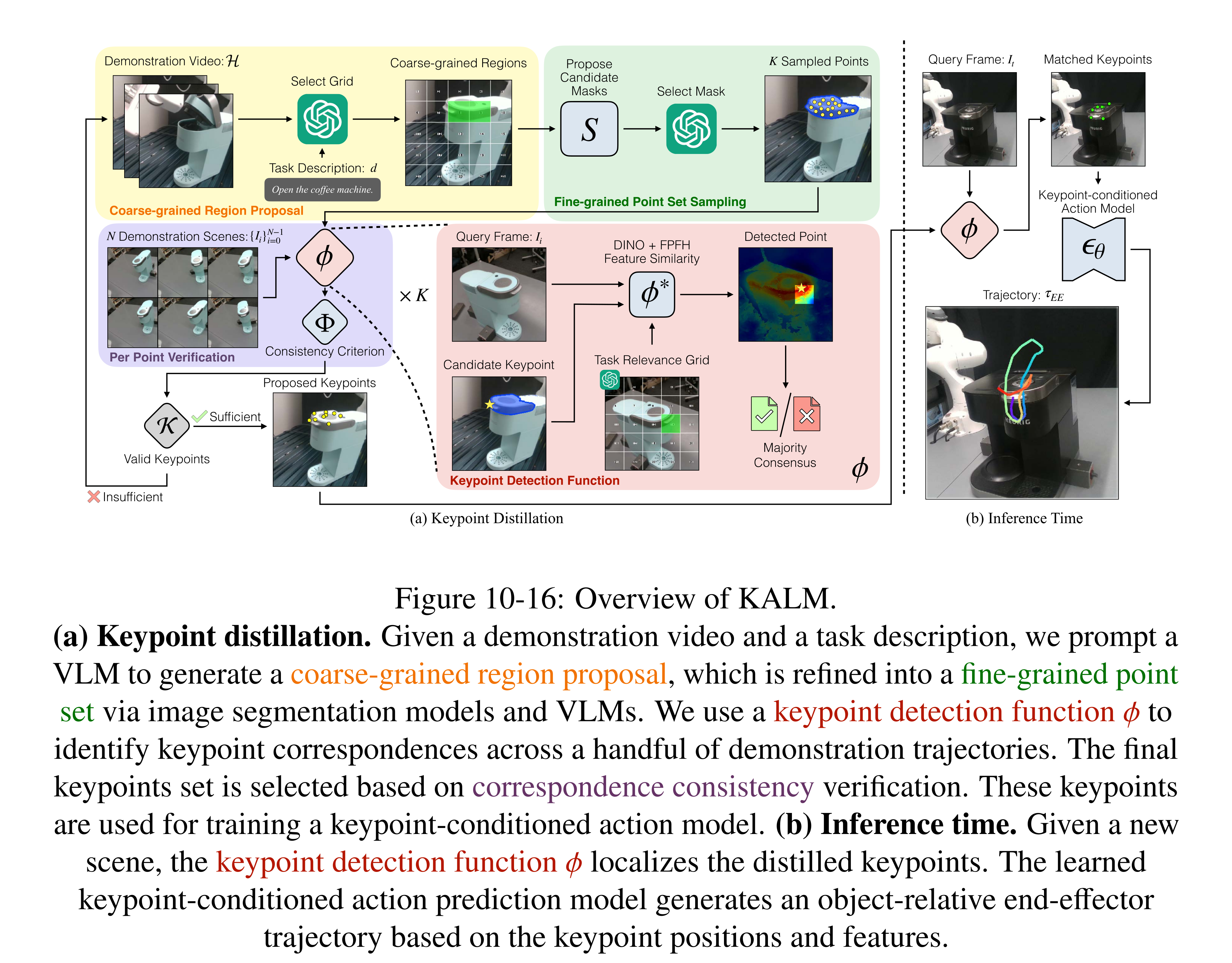
Figure 10-16: Overview of KALM. (a) Keypoint distillation. Given a demonstration video and a task description, we prompt a VLM to generate a coarse-grained region proposal, which is refined into a fine-grained point set via image segmentation models and VLMs. We use a keypoint detection function ϕ to identify keypoint correspondences across a handful of demonstration trajectories. The final keypoints set is selected based on correspondence consistency verification. These keypoints are used for training a keypoint-conditioned action model. (b) Inference time. Given a new scene, the keypoint detection function ϕ localizes the distilled keypoints. The learned keypoint-conditioned action prediction model generates an object-relative end-effector trajectory based on the keypoint positions and features.
Problem Formulation
Each skill provides initial calibrated RGB-D observations and robot trajectories. The execution segment is separated from the approach; a diffusion model learns only execution, while motion planning handles approach. Segmentation can use proximity to keypoints or trajectory statistics. These preprocessing and calibration assumptions are part of the few-demonstration setting.
Keypoint Desiderata
Useful keypoints must be task-relevant and consistently detectable across views, poses and object instances. The VLM judges relevance; feature matching across demonstrations tests consistency. Consistency is an operational correspondence test, not independent proof of semantic relevance or complete physical sufficiency.
Keypoint Proposal and Verification
A VLM selects grid regions, SAM proposes masks, and a second VLM query selects a task-related part. Farthest-point sampling proposes 3D keypoints. Matching combines feature similarity with a coarse-region preference; eight nearby points within 2cm test local consensus. A candidate must match in at least 70% of demonstrations (δ=0.3), and enough candidates must pass before the proposal is accepted. Otherwise the algorithm re-prompts. The listed loop has no explicit fixed retry bound.
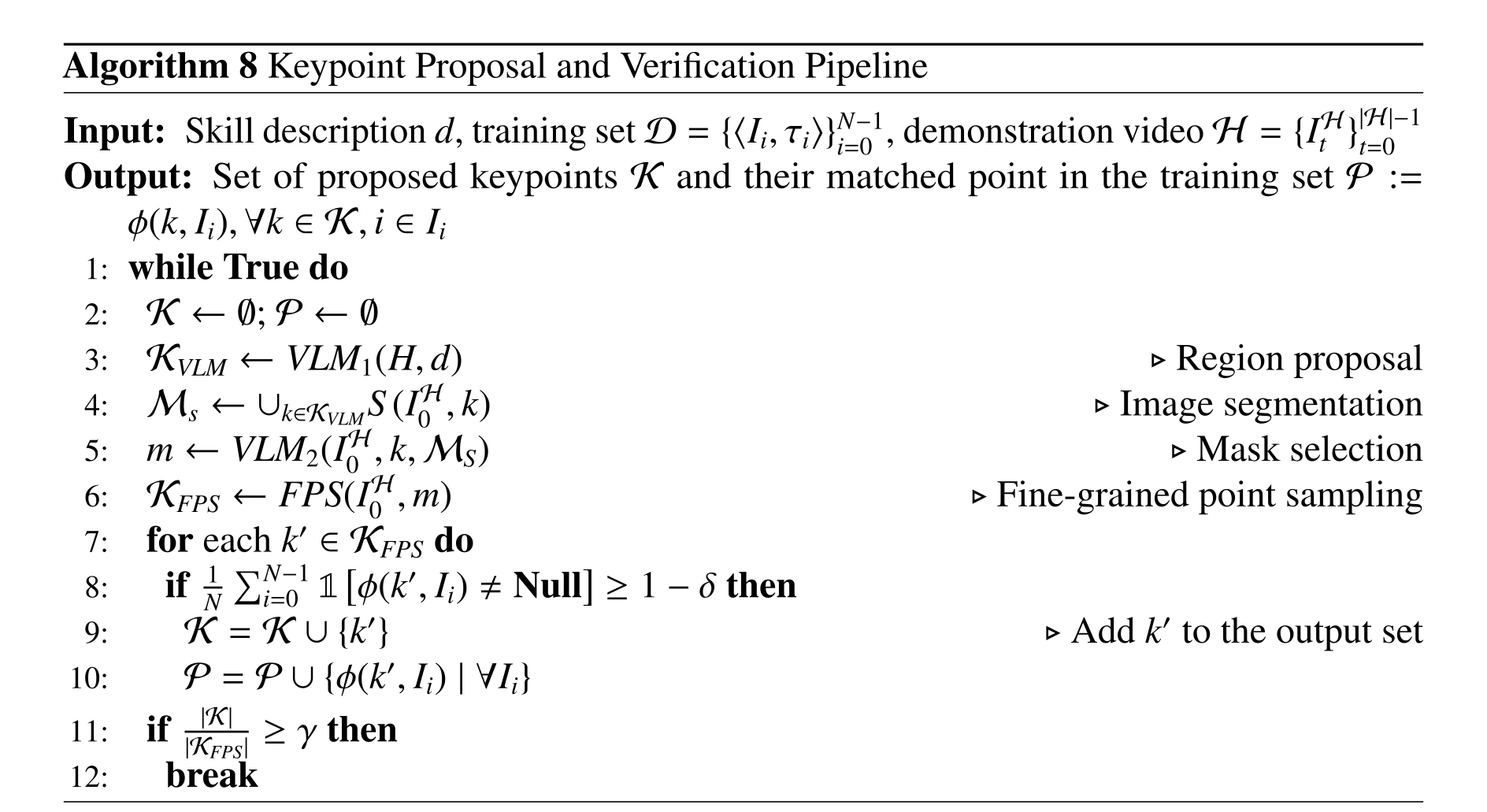
Equations


Learning Keypoint-Centric Trajectory Prediction Models
A trajectory-level Diffuser predicts end-effector poses from sparse keypoint locations/features. Coordinates are centered on the keypoints, but their axes remain aligned with the robot base. This removes absolute translation and helps camera/pose generalization; it does not mathematically impose arbitrary rotation invariance.
Implementation
The implementation uses GPT-4o, SAM, DINO/FeatUp image features and FPFH geometry. Correspondence similarities use weights 0.75 for visual and 0.25 for geometric features. The policy predicts 48 end-effector poses using a standard diffusion loss conditioned on the unordered keypoint set.
Equation

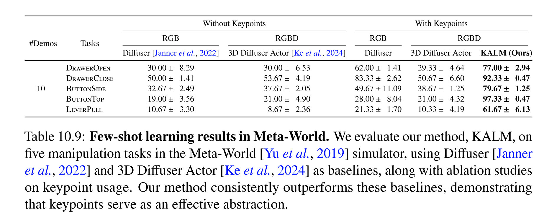
Table 10.9: Few-shot learning results in Meta-World. We evaluate our method, KALM, on five manipulation tasks in the Meta-World [Yu et al., 2019] simulator, using Diffuser [Janner et al., 2022] and 3D Diffuser Actor [Ke et al., 2024] as baselines, along with ablation studies on keypoint usage. Our method consistently outperforms these baselines, demonstrating that keypoints serve as an effective abstraction.
Inference-time Pipeline
At test time, detect the stored keypoints, sample an execution trajectory, and seek a collision-free approach to its initial pose. If approach planning fails, resample. The described feasibility check concerns reaching the trajectory start; it should not be inflated into a formal safety guarantee for every learned execution point.
Simulation Experiments in Meta-World
Five Meta-World tasks randomize object/camera poses but use manually specified oracle keypoints, with initially occluded views excluded. Thus simulation isolates representation/data efficiency rather than validating automatic discovery. With ten demonstrations, KALM scores 77.0%, 92.33%, 79.67%, 97.33% and 61.67%, outperforming the listed image/point-cloud baselines; each result uses 100 episodes and three seeds. The 10–500 demonstration study finds KALM near peak by 100, while 3D Diffuser Actor needs about 500 for competitive results.
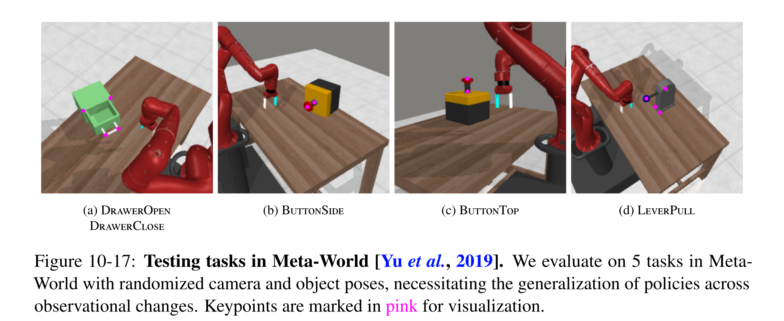
Figure 10-17: Testing tasks in Meta-World [Yu et al., 2019]. We evaluate on 5 tasks in Meta- World with randomized camera and object poses, necessitating the generalization of policies across observational changes. Keypoints are marked in pink for visualization.
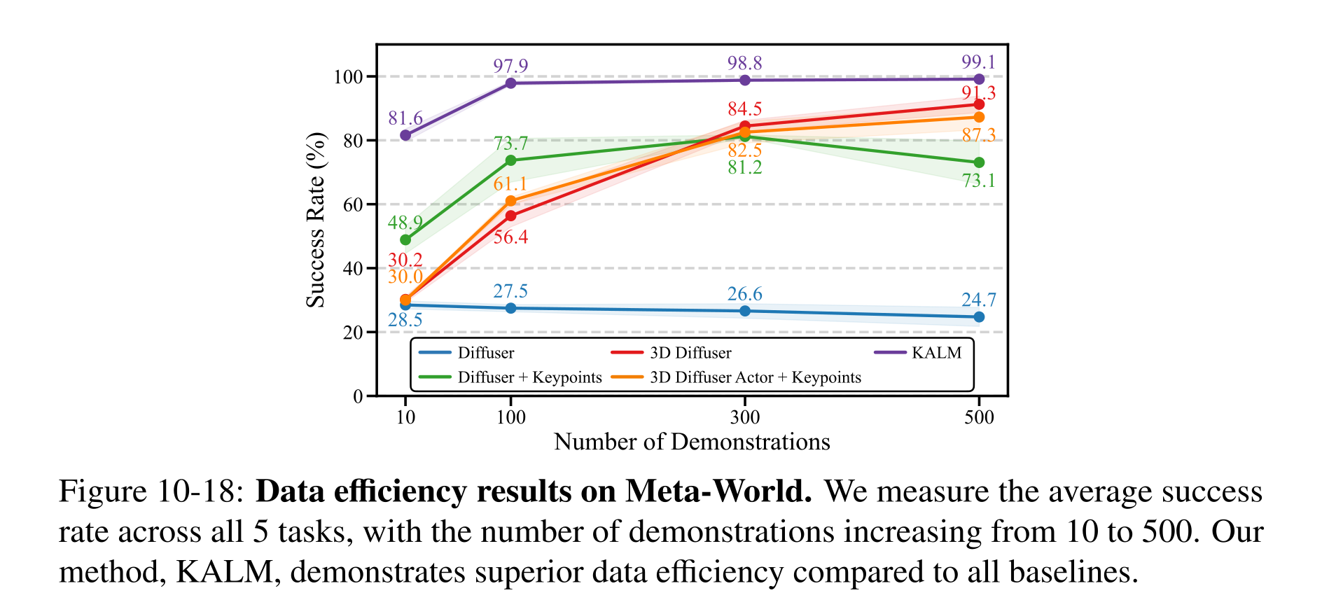
Figure 10-18: Data efficiency results on Meta-World. We measure the average success rate across all 5 tasks, with the number of demonstrations increasing from 10 to 500. Our method, KALM, demonstrates superior data efficiency compared to all baselines.
Real-World Experiments on Franka Arm
Three Franka tasks—coffee-machine handle lifting, drawer opening and spoon-to-bowl pouring—use ten demonstrations each and a gripper-mounted RGB-D camera. In ten matched test setups per condition, verified keypoints yield 9/10, 6/10 and 8/10 under view/pose variation and 6/10, 7/10 and 6/10 on unseen objects. Direct VLM selection without consistency verification is markedly worse. This small real-world comparison tests the verification pipeline; full Diffuser/3D Diffuser Actor baselines were not trained and compared here.
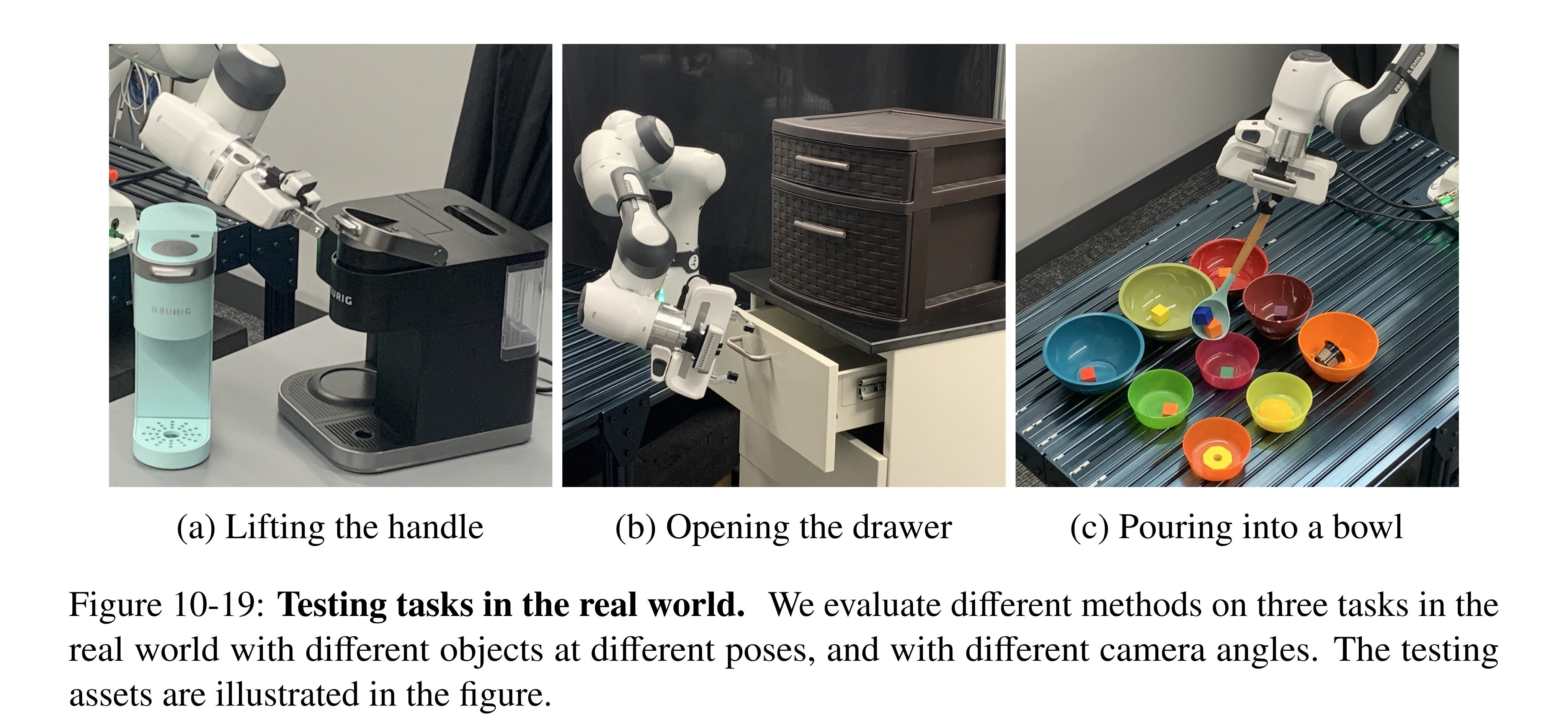
Figure 10-19: Testing tasks in the real world. We evaluate different methods on three tasks in the real world with different objects at different poses, and with different camera angles. The testing assets are illustrated in the figure.
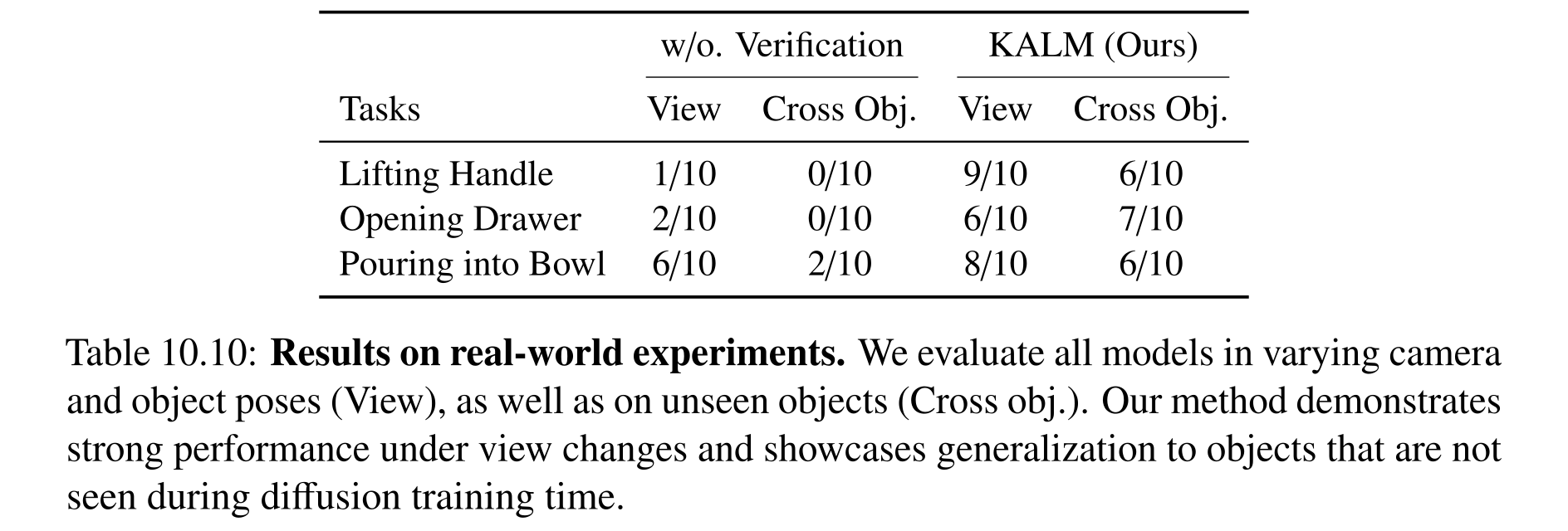
Table 10.10: Results on real-world experiments. We evaluate all models in varying camera and object poses (View), as well as on unseen objects (Cross obj.). Our method demonstrates strong performance under view changes and showcases generalization to objects that are not seen during diffusion training time.
Related Work
The chapter connects contact-space task-and-motion planning, learned tool affordances, object/part/keypoint abstractions, correspondence learning and VLM-generated robot actions. Its distinctions are reusable contact macros, visual-plus-geometric analogy, and verified automatic keypoint selection. Claims of no extra task-specific data should be read separately from the mechanisms’ simulator self-play and the substantial upstream pretraining used by MAGIC/KALM.
Discussion
The unifying result is that structured contact and keypoint representations can focus search and improve learning from limited demonstrations. Remaining scope includes known object/state models, canonical reduced-dimensional contact geometry, simulator fidelity and imperfect correspondence detection. Multi-contact/multi-agent generalization, richer physical abstractions and tighter integration with language-guided planning are future directions rather than demonstrated capabilities.
Neuro-Symbolic Long-Horizon Planning
PDSketch combines human-specified locality/sparsity with learned state features, predicate meanings and dynamics; a planner then composes actions for new logical goals. BLADE acquires Boolean action descriptions from language-annotated demonstrations and LLM proposals, learns their visual grounding and control policies, and replans during execution. Both rely on structured models, but differ in which structures humans supply.
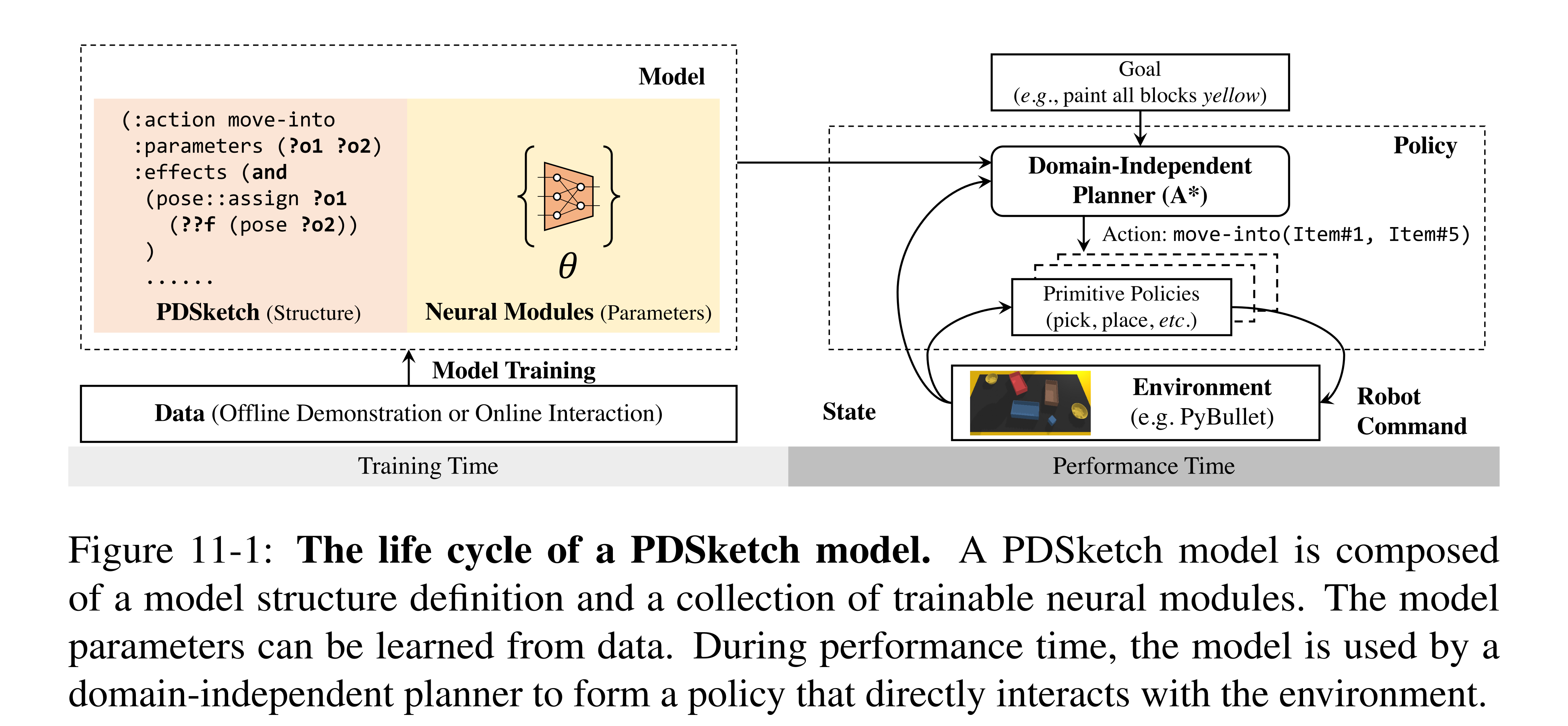
Figure 11-1: The life cycle of a PDSketch model. A PDSketch model is composed of a model structure definition and a collection of trainable neural modules. The model parameters can be learned from data. During performance time, the model is used by a domain-independent planner to form a policy that directly interacts with the environment.
Introduction
Factoring state and action effects by objects and attributes can make learning and planning easier: picking changes a few poses, not every object property. PDSketch exposes these priors as a programmable model sketch. BLADE reduces manual action-model specification using language and demonstrations, while still using a supplied predicate-name vocabulary in its main implementation.
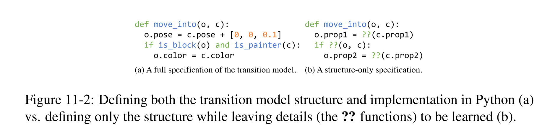
Figure 11-2: Defining both the transition model structure and implementation in Python (a) vs. defining only the structure while leaving details (the ?? functions) to be learned (b).
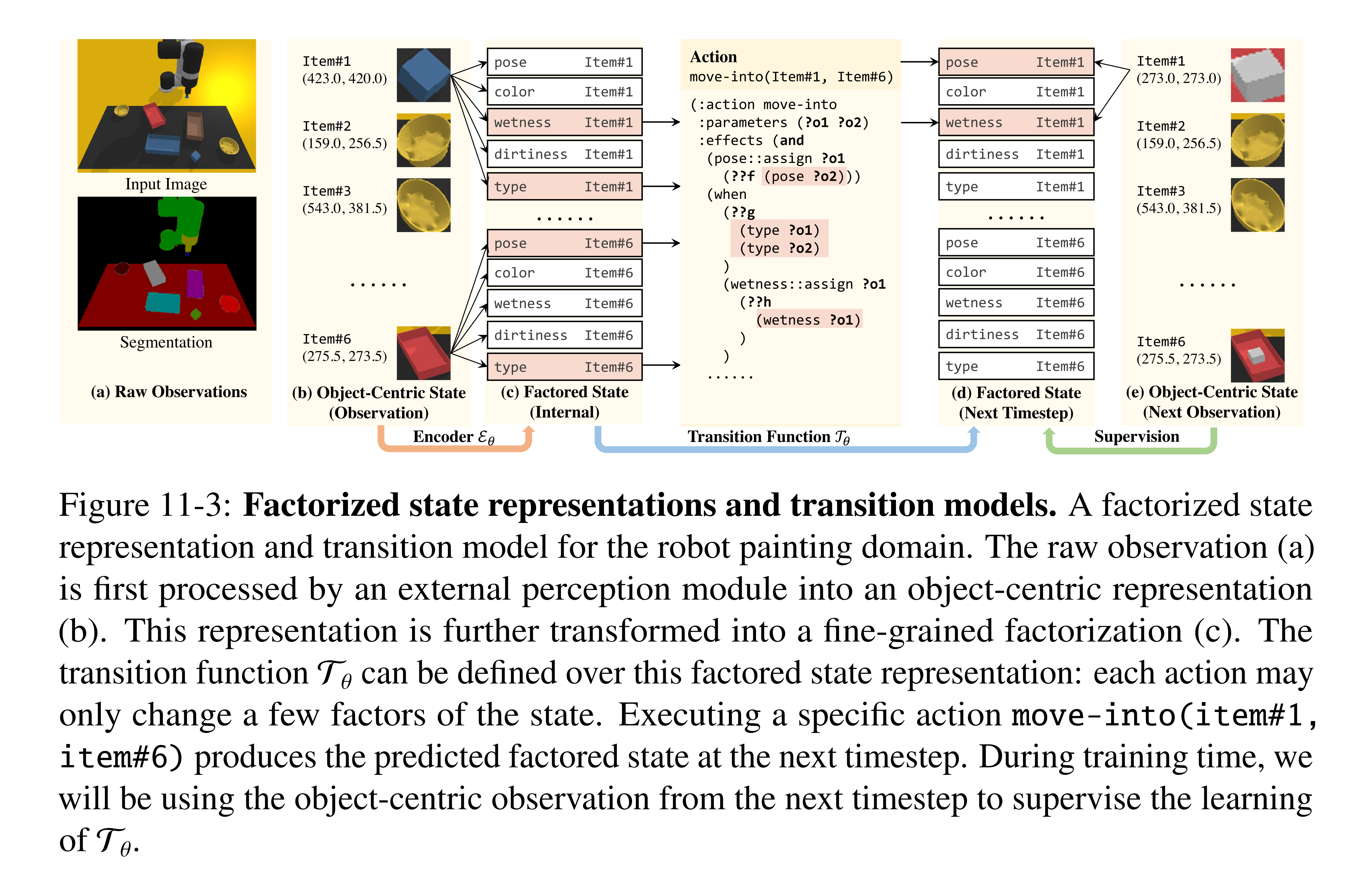
Figure 11-3: Factorized state representations and transition models. A factorized state representation and transition model for the robot painting domain. The raw observation (a) is first processed by an external perception module into an object-centric representation (b). This representation is further transformed into a fine-grained factorization (c). The transition function 𝒯θ can be defined over this factored state representation: each action may only change a few factors of the state. Executing a specific action move-into(item#1, item#6) produces the predicted factored state at the next timestep. During training time, we will be using the object-centric observation from the next timestep to supervise the learning of 𝒯θ.
PDSketch
Training data contain state/action trajectories, logical goals and per-state goal-satisfaction labels. A shared parameter set learns a latent encoder, goal evaluator and deterministic transition model. Objects are detected/tracked externally and remain fixed within an episode; actions are assumed to have sparse, local effects, with available primitive controllers. Mild stochasticity/partial observability is approximated by a deterministic latent model rather than explicitly solved as a general belief-state problem.
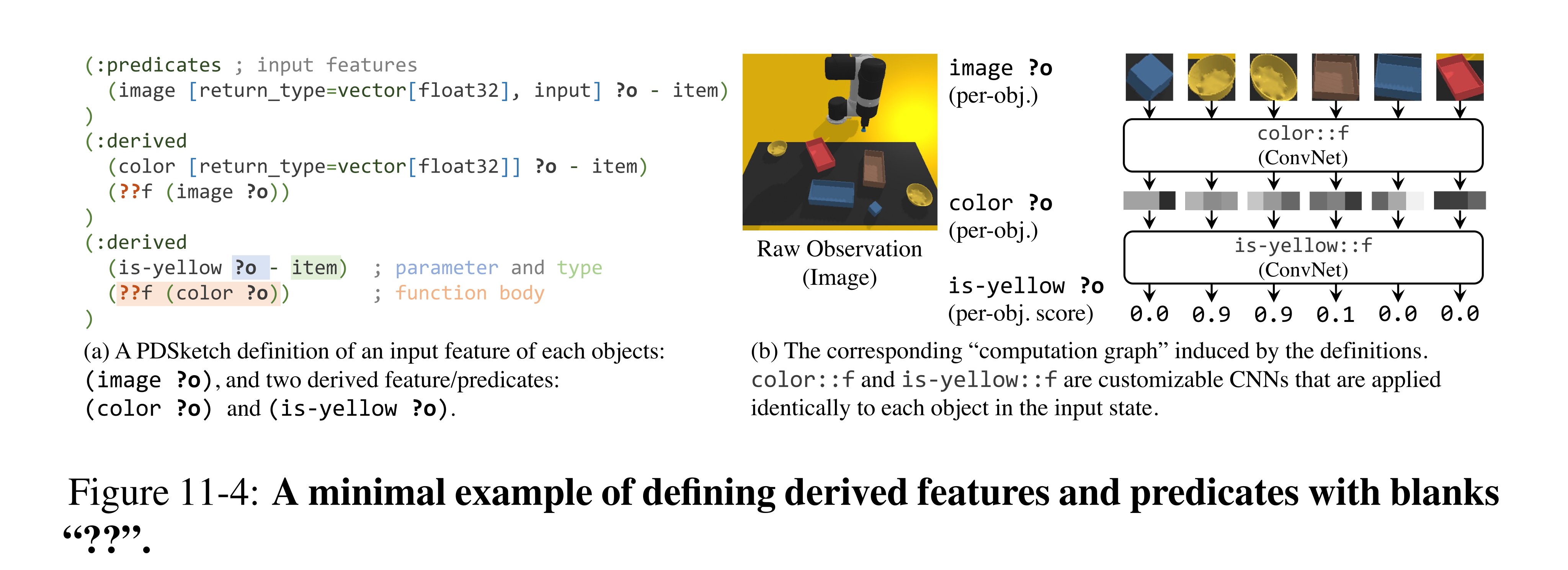
Figure 11-4: A minimal example of defining derived features and predicates with blanks “??”.
Representation Language
PDSketch extends PDDL with vector-valued features and neural-network blanks. A sketch states which properties an effect depends on and changes, while neural modules learn the actual functions. Conditional updates are softened to differentiable mixtures, and finite-domain first-order logic supports relational and quantified goals. Added structure is a human inductive bias, not automatically inferred in this system.
Model Learning and Planning with PDSketch
Learning combines binary goal-satisfaction loss, one-step latent transition error and a lookahead term to discourage degeneracy. Shared predicate networks and soft Gödel logic make the assembled computation graph trainable. Forward search applies the learned transition model; a node counts as a goal when its evaluator exceeds 0.5. Planning correctness is relative to that learned model and evaluator, so model error can still cause physical failure.
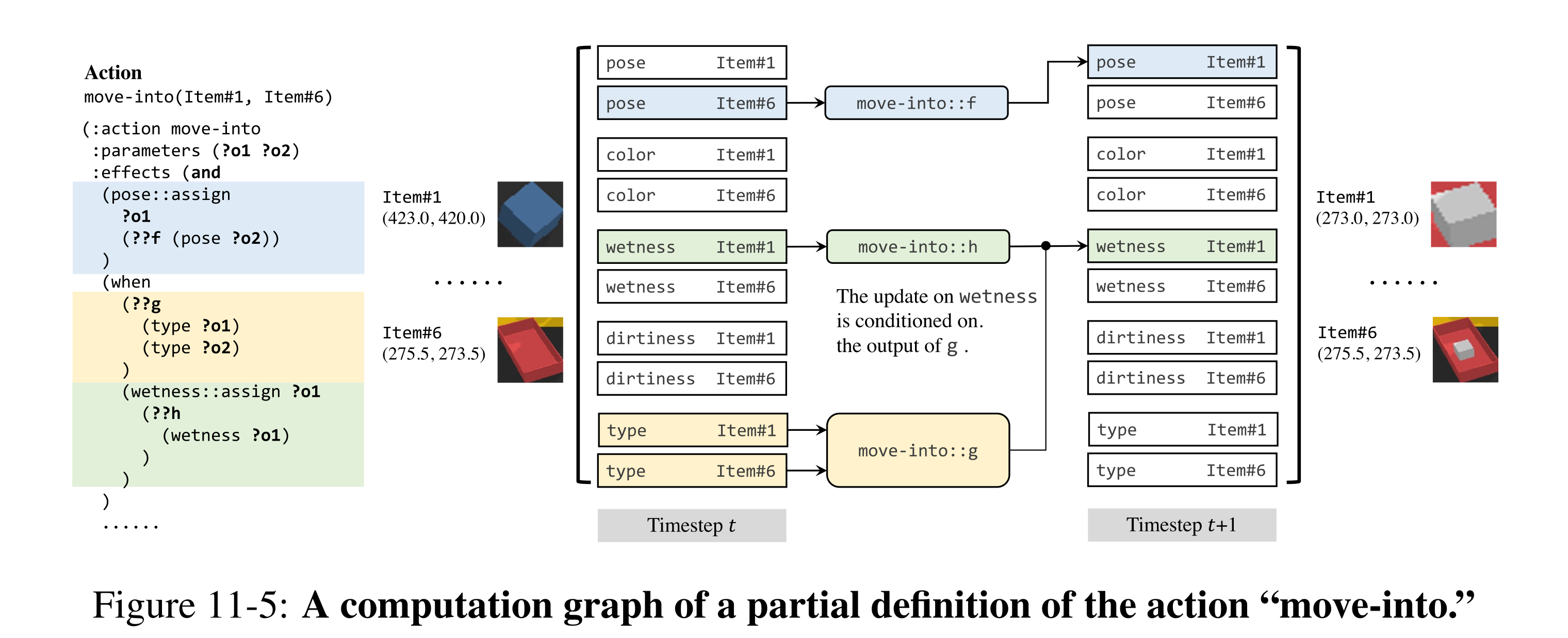
Figure 11-5: A computation graph of a partial definition of the action “move-into.”
Equation

Inducing Domain-Independent Heuristics
To derive an hFF-style heuristic, vector features are quantized and external neural functions approximated by first-order decision trees. A relaxed problem allows predicates to retain multiple values simultaneously, yielding an inexpensive goal-distance estimate. Quantization is used only for guidance; forward simulation keeps the original learned model. This separation avoids executing a discretized model, but neither learned-model accuracy nor shortest-plan optimality follows automatically from the heuristic.
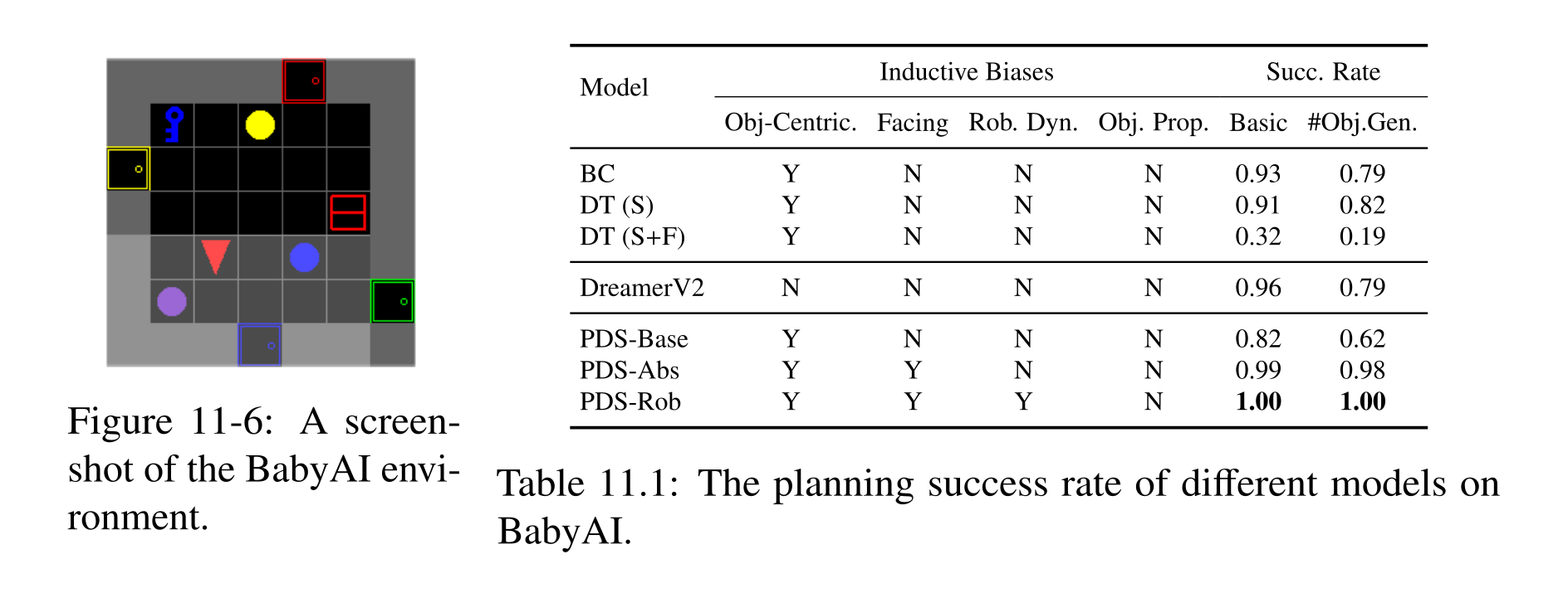
Figure 11-6: A screen- shot of the BabyAI envi- ronment.
Table 11.1: The planning success rate of different models on BabyAI.
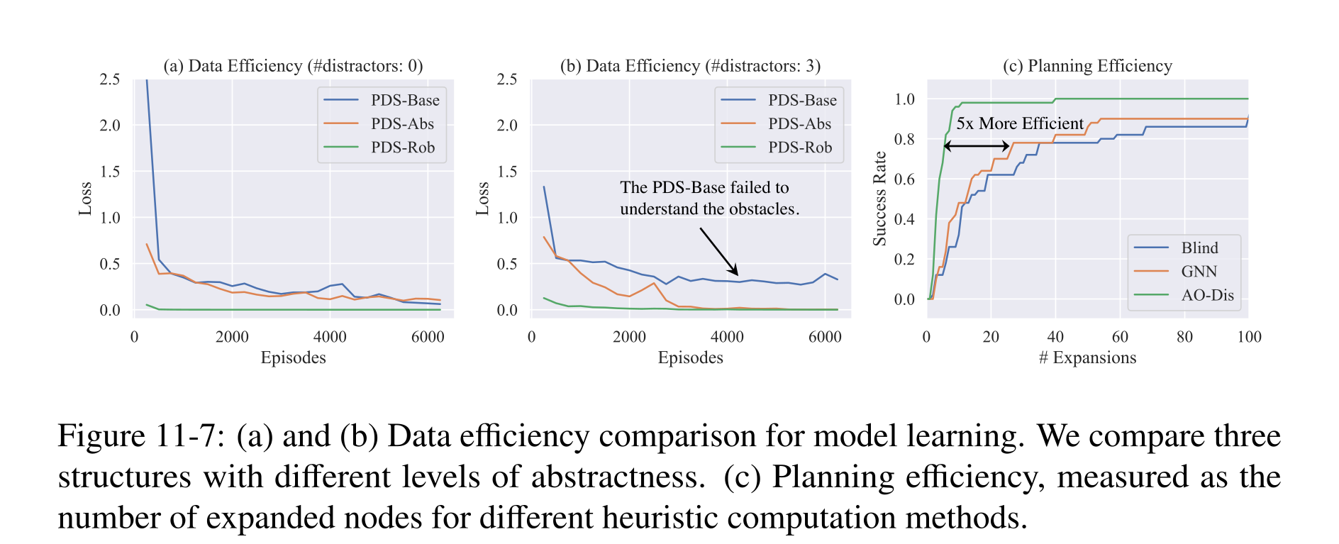
Figure 11-7: (a) and (b) Data efficiency comparison for model learning. We compare three structures with different levels of abstractness. (c) Planning efficiency, measured as the number of expanded nodes for different heuristic computation methods.
Experiments
Evaluations compare structured planning with behavior cloning, decision transformers and a model-based reinforcement-learning baseline in BabyAI, then with imitation baselines in a simulated painting domain. The amount of manually supplied model structure varies deliberately across PDSketch ablations.
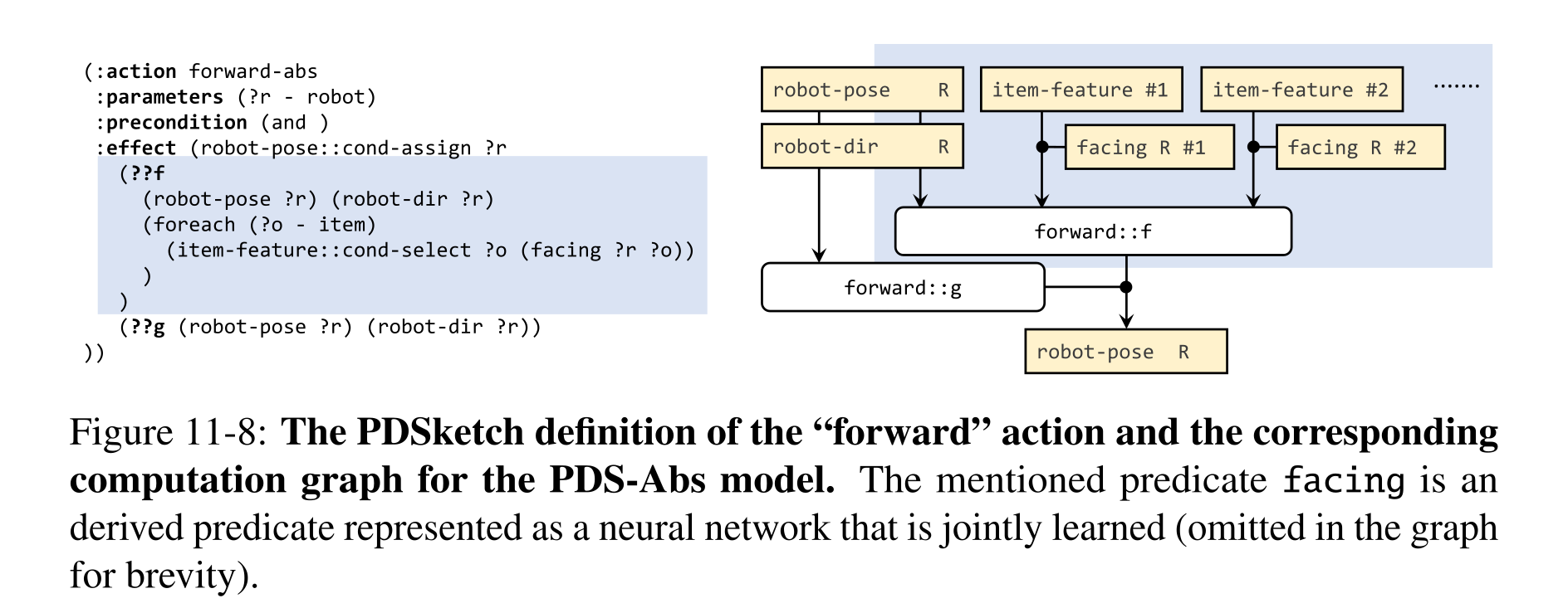
Figure 11-8: The PDSketch definition of the “forward” action and the corresponding computation graph for the PDS-Abs model. The mentioned predicate facing is an derived predicate represented as a neural network that is jointly learned (omitted in the graph for brevity).
BabyAI
BabyAI training uses a 7×7 grid with four doors/four objects, while generalization has six doors/eight objects. Basic/object-count-generalization success is 0.82/0.62 for the unstructured object-centric PDS-Base, 0.99/0.98 after adding the ungrounded facing relation and pose/appearance structure, and 1.00/1.00 with predefined robot motion rules. Behavior cloning reaches 0.93/0.79 and DreamerV2 0.96/0.79. Thus the strongest result includes additional human dynamics knowledge.
The derived heuristic expands about five times fewer nodes than the learned GNN heuristic at 80% success. This is a search-expansion comparison, not a universal fivefold wall-clock gain. The explanations for decision-transformer failure with mixed successful/failed data and for Dreamer generalization are hypotheses, not isolated causal findings.
Robot Painting
Painting uses object images/poses, learned color/state concepts, and two prebuilt pick/place primitives; one places into a specified container and the other moves to an xyz location while ignoring rotation. With 100/1,000 demonstrations, PDSketch obtains 0.91/0.99 success versus 0.70/0.95 for behavior cloning and 0.56/0.97 for the decision transformer. Three novel logical-goal families score 0.99, 0.98 and 0.87, with stacking limited by controller/physics noise. These are simulated manipulations with supplied object observations/controllers, not raw-pixel autonomous skill discovery.
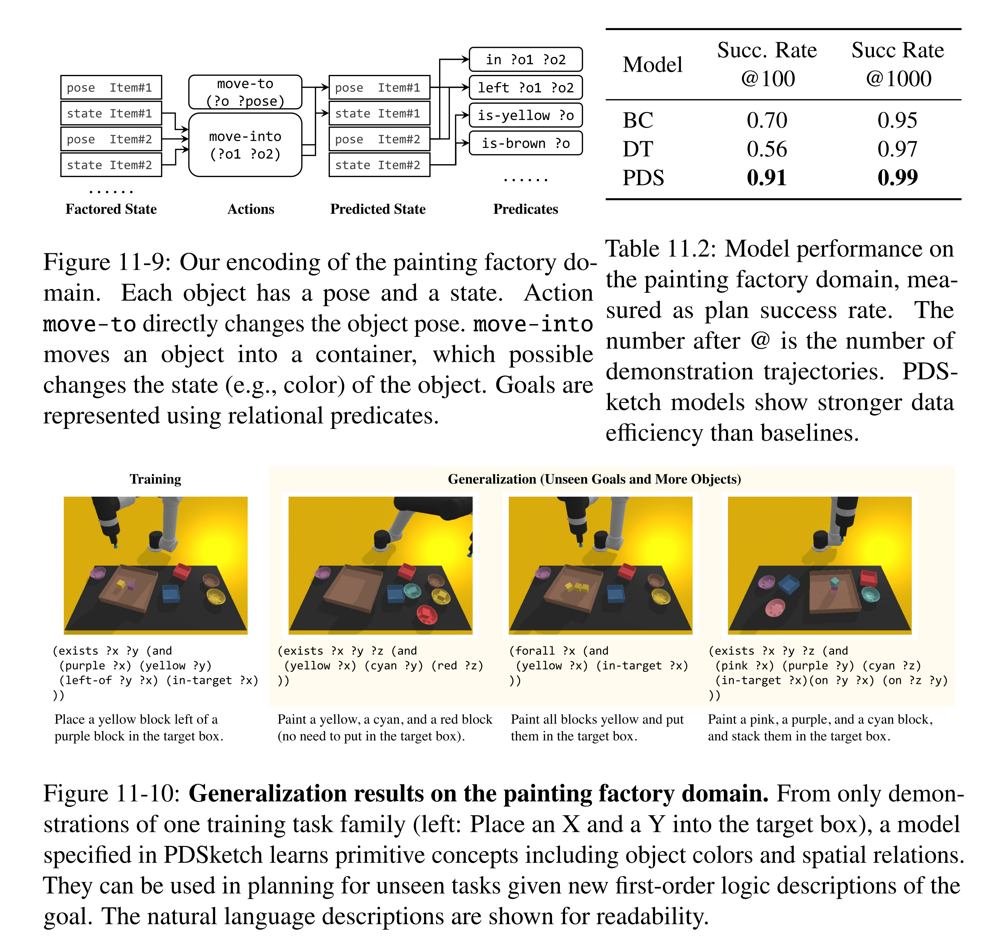
Figure 11-9: Our encoding of the painting factory do- main. Each object has a pose and a state. Action move-to directly changes the object pose. move-into moves an object into a container, which possible changes the state (e.g., color) of the object. Goals are represented using relational predicates.
Table 11.2: Model performance on the painting factory domain, mea- sured as plan success rate. The number after @ is the number of demonstration trajectories. PDS- ketch models show stronger data efficiency than baselines.
Figure 11-10: Generalization results on the painting factory domain. From only demon- strations of one training task family (left: Place an X and a Y into the target box), a model specified in PDSketch learns primitive concepts including object colors and spatial relations. They can be used in planning for unseen tasks given new first-order logic descriptions of the goal. The natural language descriptions are shown for readability.
Behavior from Language and Demonstration
BLADE learns propositional preconditions/effects and associated visual classifiers/policies from language-annotated demonstrations. Contact segmentation constrains LLM-generated descriptions; an abstract consistency check rejects incompatible proposals. The learned behavior library supports novel compositions, geometric preconditions and replanning after disturbances.
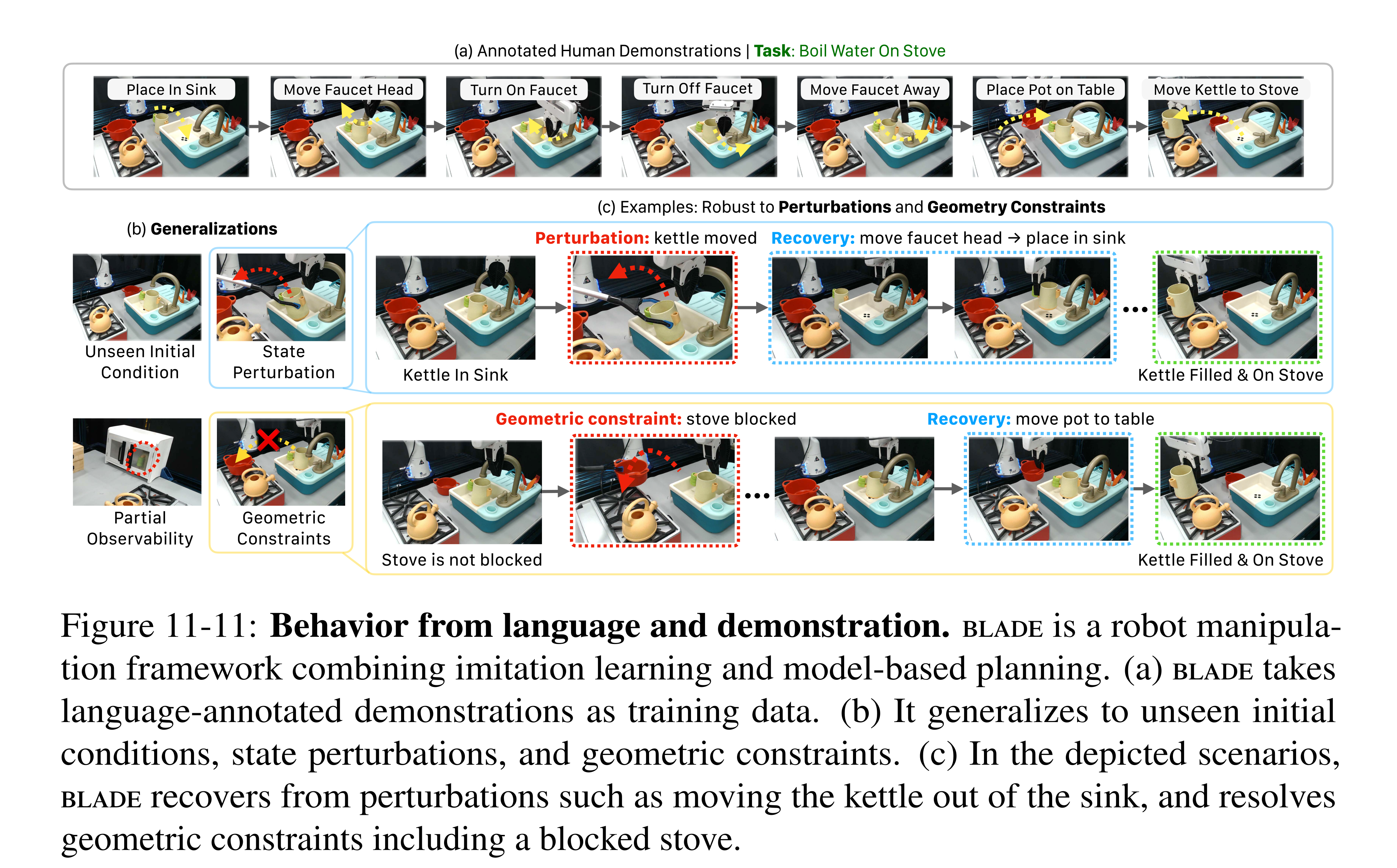
Figure 11-11: Behavior from language and demonstration. blade is a robot manipula- tion framework combining imitation learning and model-based planning. (a) blade takes language-annotated demonstrations as training data. (b) It generalizes to unseen initial conditions, state perturbations, and geometric constraints. (c) In the depicted scenarios, blade recovers from perturbations such as moving the kettle out of the sink, and resolves geometric constraints including a blocked stove.
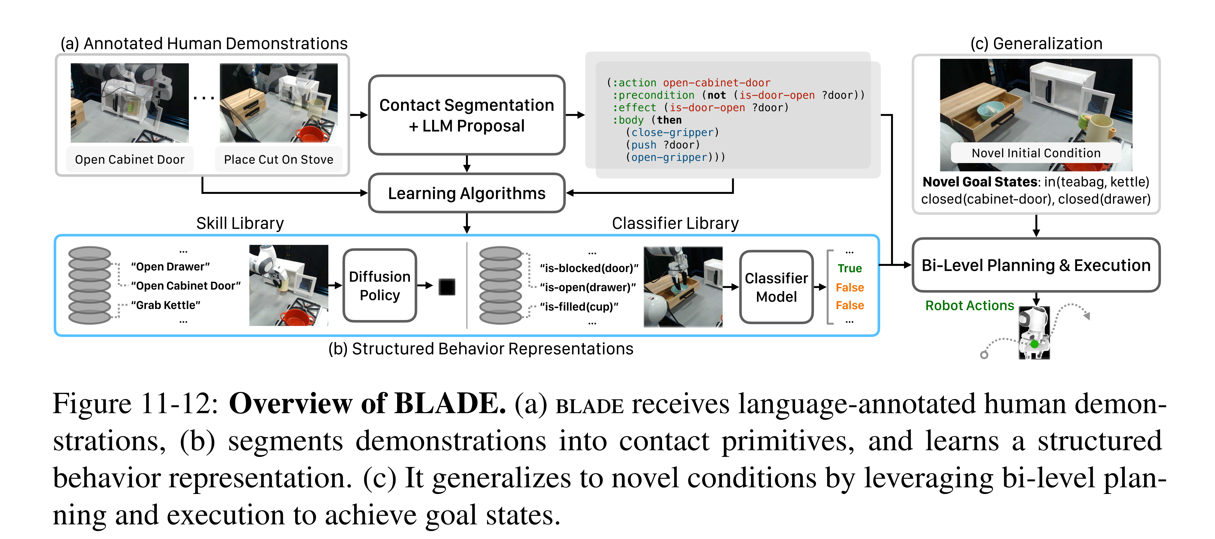
Figure 11-12: Overview of BLADE. (a) blade receives language-annotated human demon- strations, (b) segments demonstrations into contact primitives, and learns a structured behavior representation. (c) It generalizes to novel conditions by leveraging bi-level plan- ning and execution to achieve goal states.
Problem Formulation
Each language-labeled demonstration segment corresponds to one of a finite set of skills. Behaviors contain arguments, Boolean preconditions/effects and a low-level policy; classifiers ground the predicates in sensory input. The main system also receives human-supplied predicate names. Its claim of no extra state labels concerns grounding supervision, not absence of all domain vocabulary or language annotation.
Behavior Description Learning
Gripper state and object segmentation split trajectories into seven contact primitives. The LLM receives environment descriptions, neighboring behavior labels, candidate contact sequences and PDDL guidance, then proposes one body sequence and precondition/effect model per skill. Demonstrations are resegmented to fit that body. Abstract verification checks whether preceding effects support later preconditions and whether contact sequences are compatible; it tests demonstrated logical consistency, not exhaustive physical correctness.
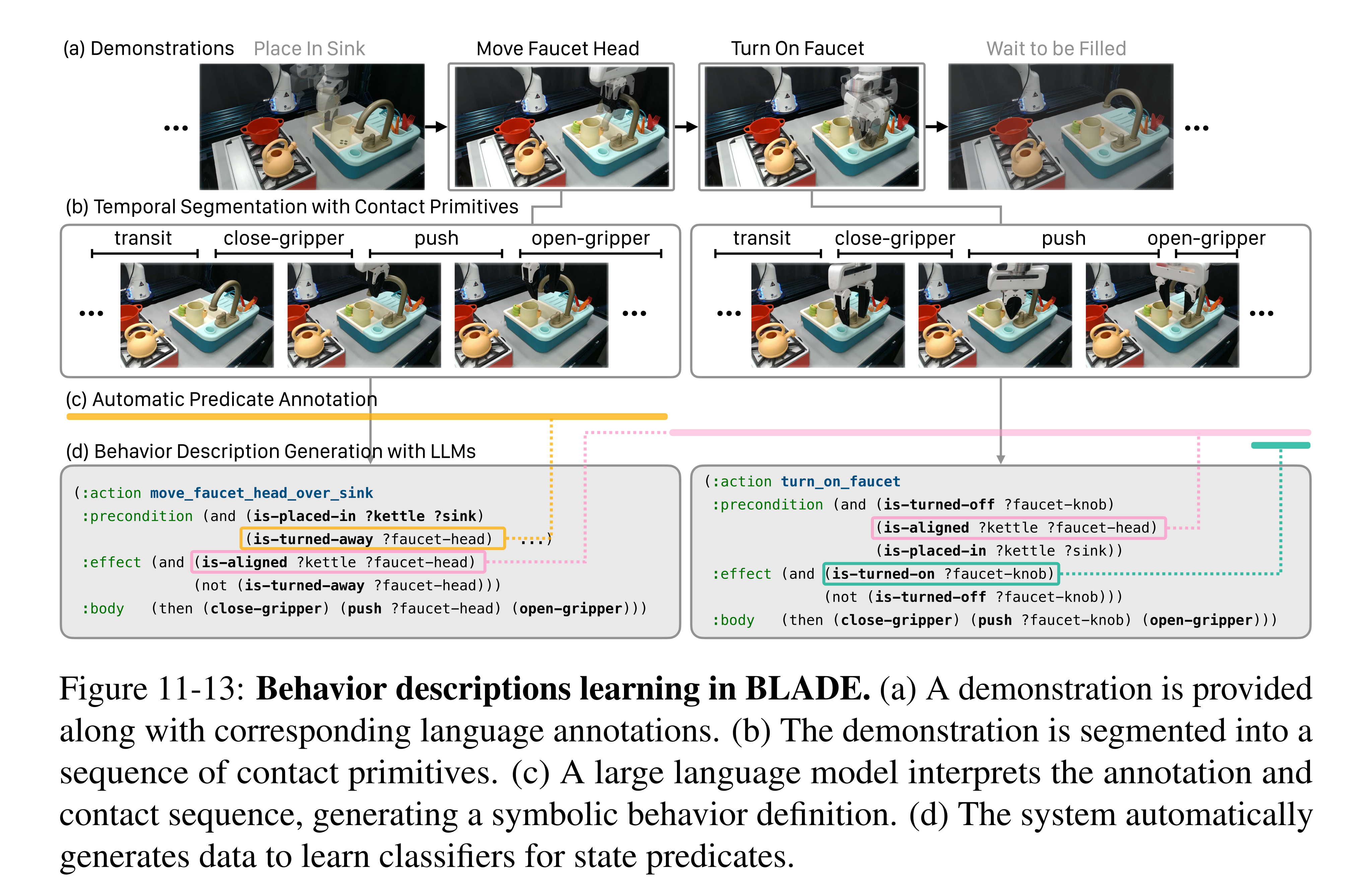
Figure 11-13: Behavior descriptions learning in BLADE. (a) A demonstration is provided along with corresponding language annotations. (b) The demonstration is segmented into a sequence of contact primitives. (c) A large language model interprets the annotation and contact sequence, generating a symbolic behavior definition. (d) The system automatically generates data to learn classifiers for state predicates.
Classifier and Policy Learning
Predicate labels are inferred from action preconditions/effects and propagated through frames until contradicted by another behavior; unknown states are left unlabeled. This enlarges supervision beyond segment endpoints, but depends on the inferred action model and frame assumptions. Neural classifiers learn these pseudo-labels, with object crops in the real-world implementation; diffusion policies learn behavior execution from camera/point-cloud observations.
Planning and Execution
An LLM translates the requested goal into predicates. Symbolic planning chooses behaviors, executes the first learned policy, then observes and replans. Visibility and blocking relations become preconditions so the planner can reveal hidden objects or move obstacles. Partial observability uses a most-likely-state assumption plus replanning; it is not probabilistic belief-space planning or a guarantee against all perturbations.
Simulation Experiments
CALVIN split D supplies roughly six hours of play and 34 behavior labels; six new composition tasks use 20 initial states each and three seeds. With learned classifiers, BLADE reaches 68.33% on abstract goals, 26.67% on geometric constraints and 75.83% on partial observability, versus HULC’s 2.78%, 11.67% and 0%. The abstract-goal difference is 65.55 percentage points, not an ambiguous 65% relative gain.
Providing ground-truth states raises abstract/geometric success to 76.11%/56.67%, but partial-observability success is 70%, below the learned-state variant; the improvement is therefore not uniform. Dense propagated predicate supervision outperforms endpoint-only supervision (33.89%, 9.17%, 3.33% planning success), supporting its practical value. Absolute geometric-constraint performance remains limited, and the reported baselines differ in representation and training requirements.
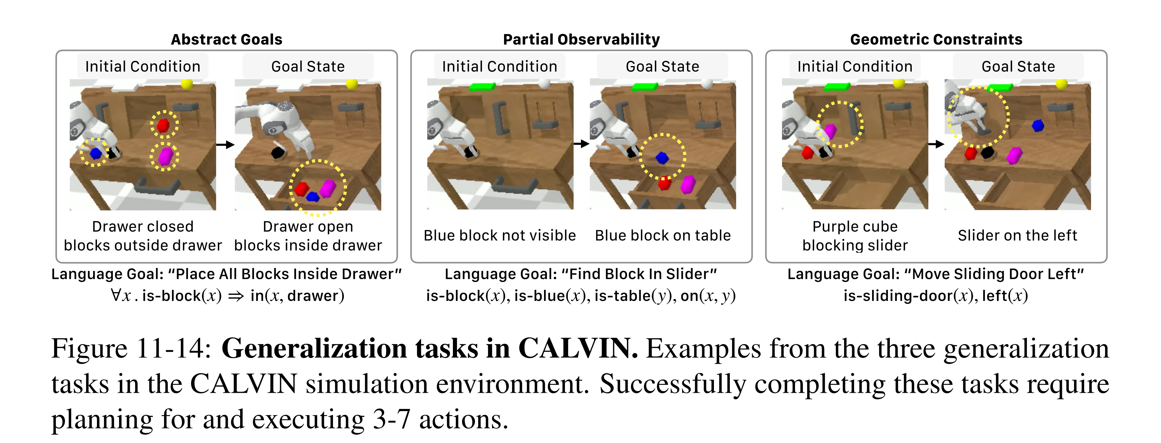
Figure 11-14: Generalization tasks in CALVIN. Examples from the three generalization tasks in the CALVIN simulation environment. Successfully completing these tasks require planning for and executing 3-7 actions.
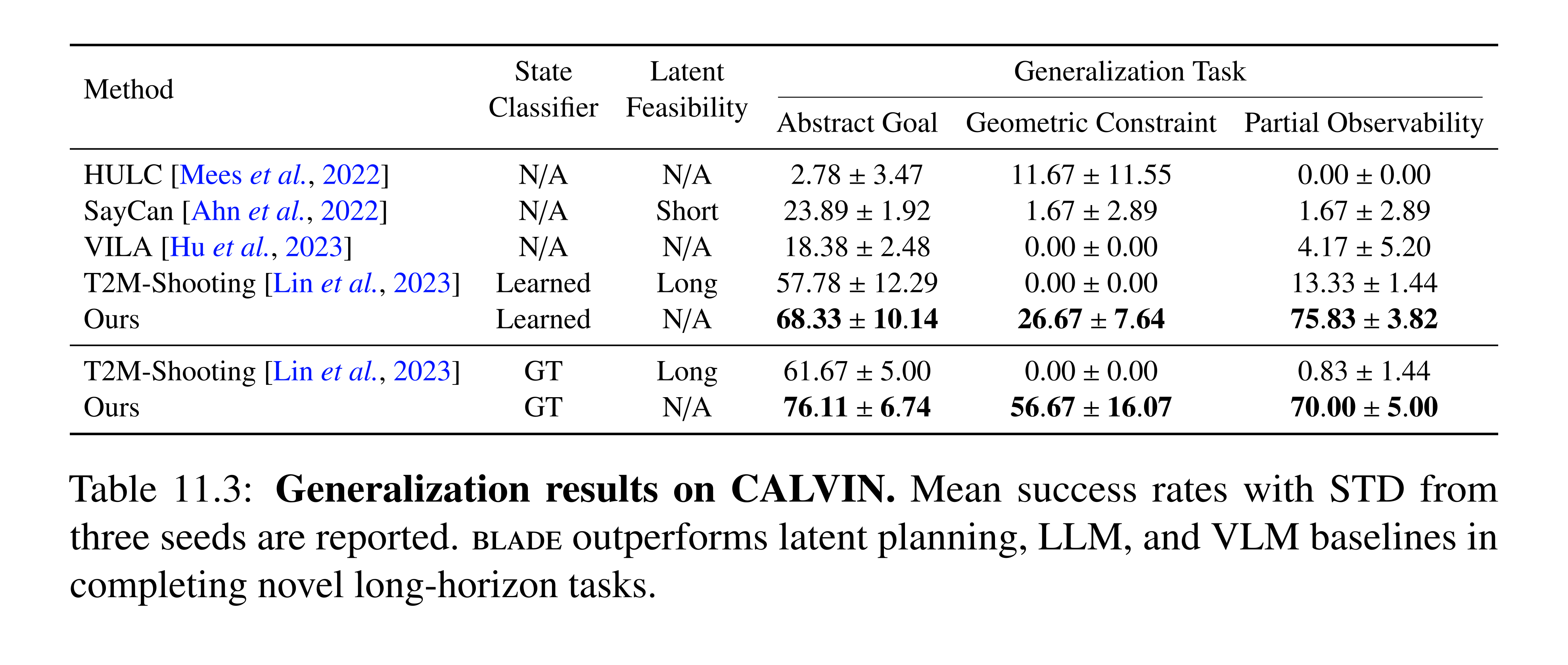
Table 11.3: Generalization results on CALVIN. Mean success rates with STD from three seeds are reported. blade outperforms latent planning, LLM, and VLM baselines in completing novel long-horizon tasks.
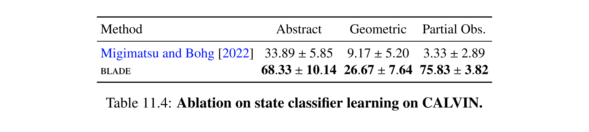
Table 11.4: Ablation on state classifier learning on CALVIN.
Real-World Experiments
Two Franka domains use five cameras and 85 language-annotated demonstrations per domain. Six tests per generalization condition compare BLADE with Robot-VILA; SayCan/Text2Motion are omitted because of additional training-data requirements. In the plotted Boil Water domain, BLADE gets 5/6 on original sequences and 6/6 on unseen starts, perturbations and geometric constraints. In Make Tea it gets 5/6 on original sequences and 4/6 in each of the four generalization conditions. Robot-VILA scores 0/6 or 1/6.
Figure 11-15’s caption swaps the prose names of the two domains; the panel labels and Appendix L correctly identify the faucet/sink setup as Boil Water and the cabinet/drawer/teabag setup as Make Tea. These small controlled tests demonstrate useful recomposition and recovery, rather than general reliability guarantees.
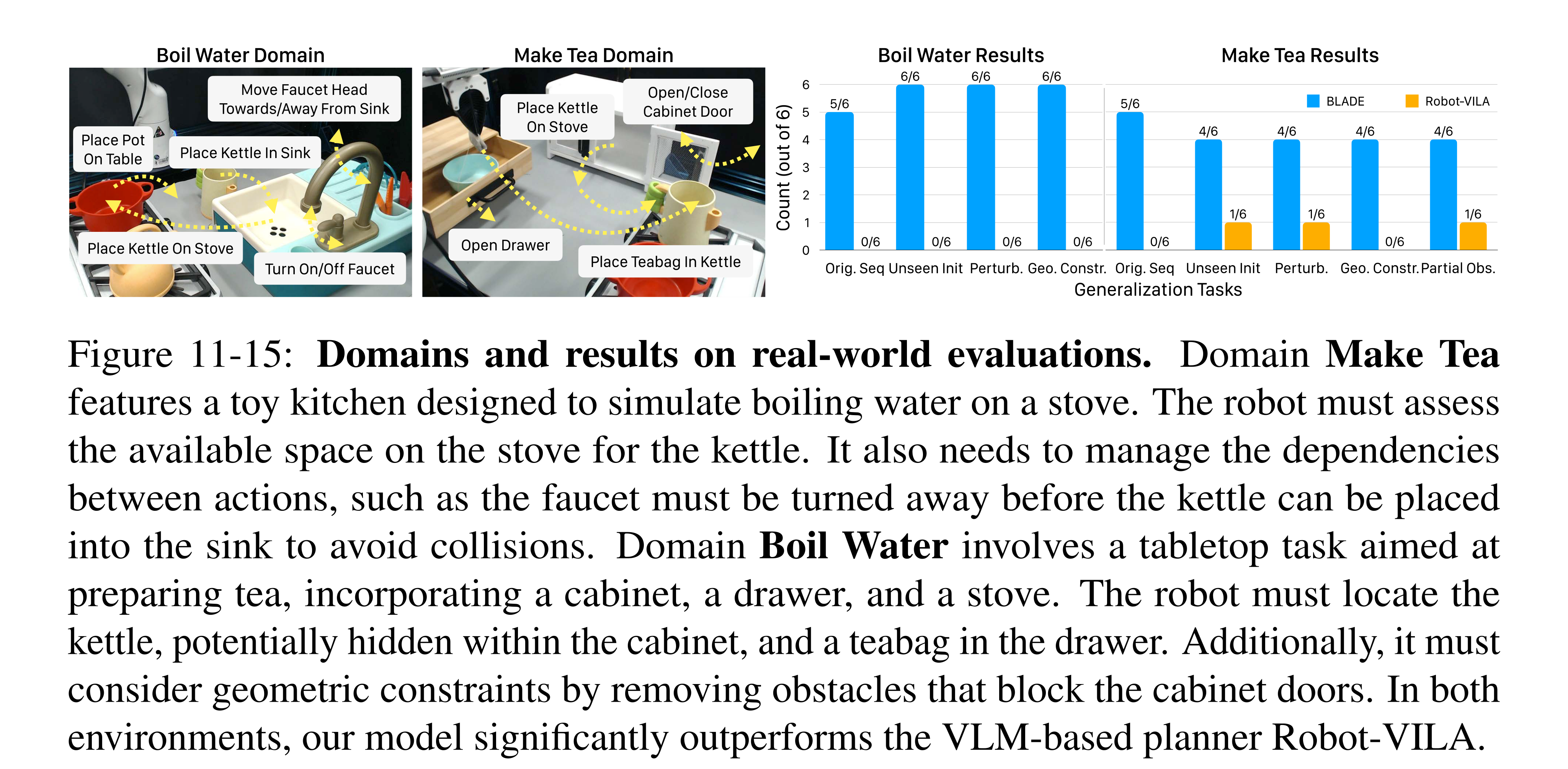
Figure 11-15: Domains and results on real-world evaluations. Domain Make Tea features a toy kitchen designed to simulate boiling water on a stove. The robot must assess the available space on the stove for the kettle. It also needs to manage the dependencies between actions, such as the faucet must be turned away before the kettle can be placed into the sink to avoid collisions. Domain Boil Water involves a tabletop task aimed at preparing tea, incorporating a cabinet, a drawer, and a stove. The robot must locate the kettle, potentially hidden within the cabinet, and a teabag in the drawer. Additionally, it must consider geometric constraints by removing obstacles that block the cabinet doors. In both environments, our model significantly outperforms the VLM-based planner Robot-VILA.
Related Work
The work connects object-factored dynamics, differentiable/neuro-symbolic programming, hierarchical skill composition and LLM-assisted planning. PDSketch makes locality/sparsity explicit while learning neural groundings; BLADE uses language-model proposals to construct grounded symbolic action models. Its advantage over direct action-text generation comes from executing a structured model with state feedback, subject to classifier and policy quality.
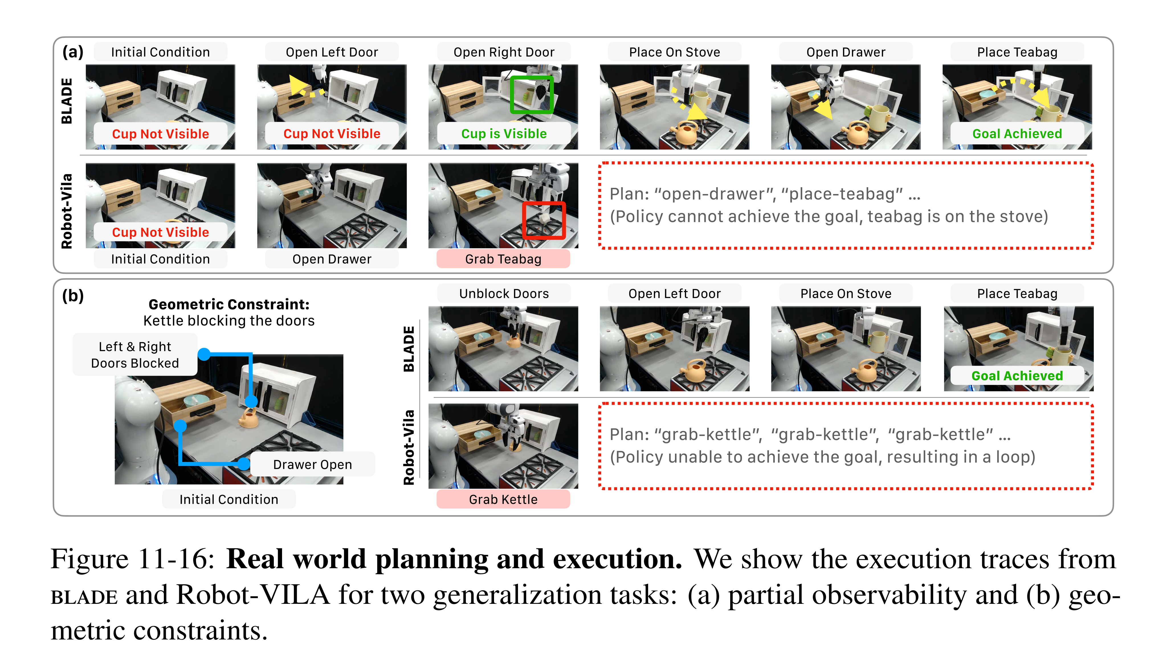
Figure 11-16: Real world planning and execution. We show the execution traces from blade and Robot-VILA for two generalization tasks: (a) partial observability and (b) geo- metric constraints.
Discussion
PDSketch shows the value of specified structure; BLADE shows a route to acquiring action dependencies from demonstrations and language. Remaining limitations include gripper-based segmentation, supplied predicate names, noisy state classification and low-level policy generalization. Open-ended predicate invention and more uncertainty-aware planning remain future work.
Hybrid Imperative-Declarative Action Representations
The Crow Definition Language (CDL) combines direct procedures with nondeterministic planning rules, continuous constraints and explicit commitments. Its interpreter, Crow, searches only where the program leaves choices open. Navigation among movable obstacles illustrates the tradeoff: restrictive strategies solve easy instances quickly, whereas harder instances need intermediate waypoints and interleaved subplans.
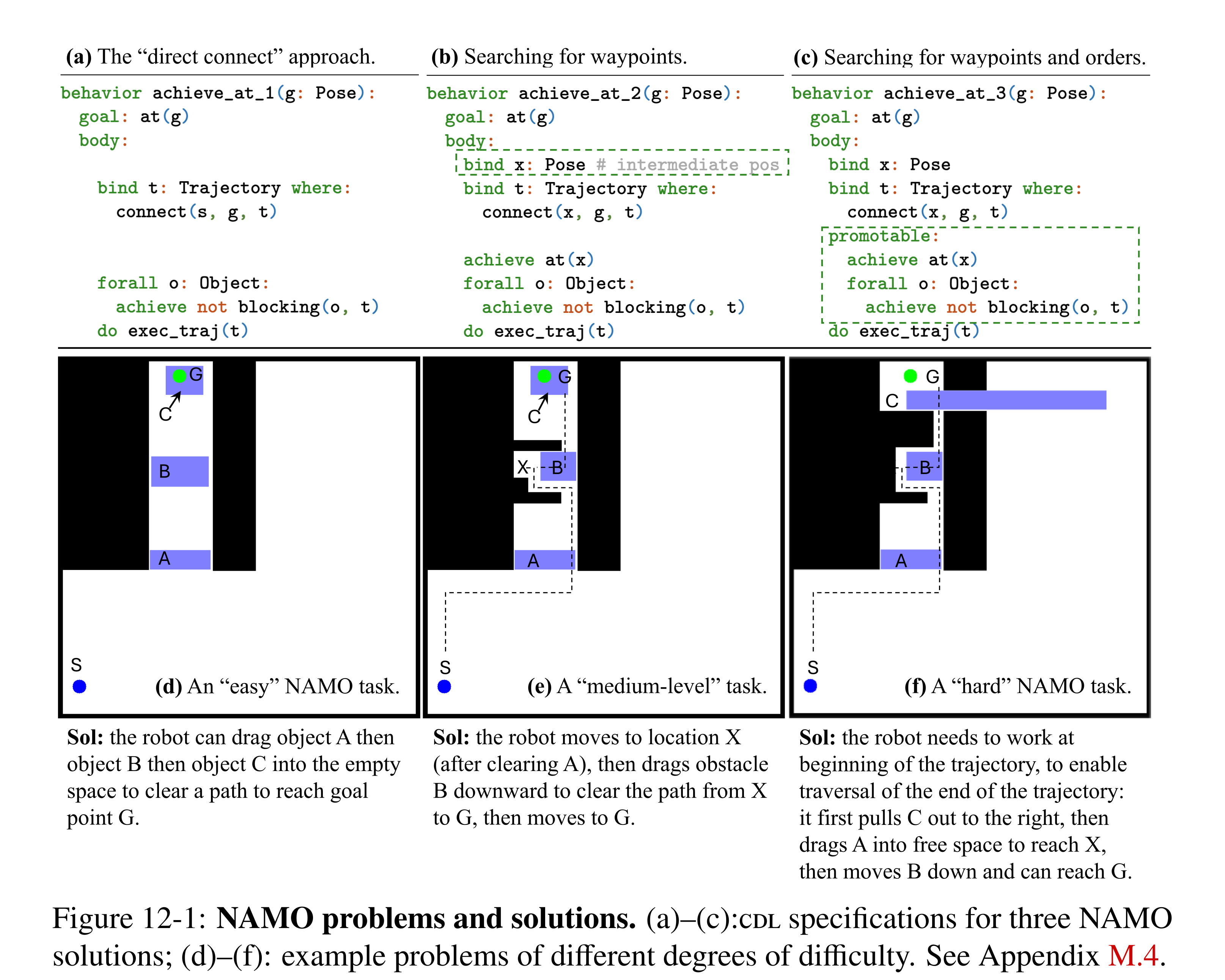
Figure 12-1: NAMO problems and solutions. (a)–(c):cdl specifications for three NAMO solutions; (d)–(f): example problems of different degrees of difficulty. See Appendix M.4.
Introduction
Imperative policies make choices directly; declarative models defer them to search. CDL describes a spectrum between these approaches through choices of behavior, subgoal order/interleaving and variable bindings. Domain knowledge can constrain those choices, but efficiency comes with assumptions about which decisions can safely be made independently.
The Crow Definition Language (CDL)
The formal setting assumes fully observable states, deterministic transitions, uniform action costs and a fixed finite entity set. Typed relational features connect external perception to behavior rules; primitive controllers implement physical actions. A rule states a goal and a program body that can generate candidate primitive plans. This chapter supplies a representation/interpreter, not an experimentally demonstrated general learned household agent.


Imperative Behavior Scripting in cdl
The imperative core uses let for deterministic computation, achieve to invoke a goal-achieving rule and do to add a primitive controller. A single method per goal yields a hierarchical program with no search over alternatives. Its correctness rests on the programmer’s rule; the simple obstacle-clearing example assumes individually movable obstacles and sufficient available storage space.



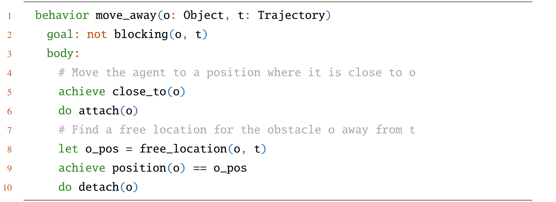
Nondeterminsitic Behaviors and Soundness Checking
Multiple methods for one goal introduce branching. Assertions constrain intermediate/final states, while effect blocks project how features change. Refinement expands achieve statements until only primitive actions, assertions and effects remain. Internal soundness means assertions hold in the projected state; it implies external goal achievement only when the final goal is asserted and rule effects agree with actual world transitions.



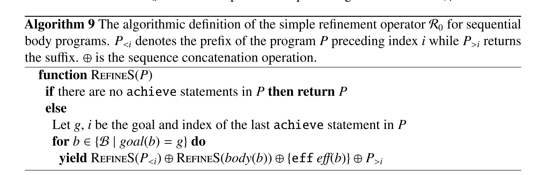
Equation

Subgoal Ordering and Promotion
Unordered groups allow subgoal reordering without interleaving their primitive solutions; promotable groups permit interleaving. A rule is partitioned into left, promotable middle and right sections. Refining a middle goal merges its own middle into the outstanding subgoals while placing its left/right requirements around them. This gives programmers finer control than permitting all subplans to interleave indiscriminately.

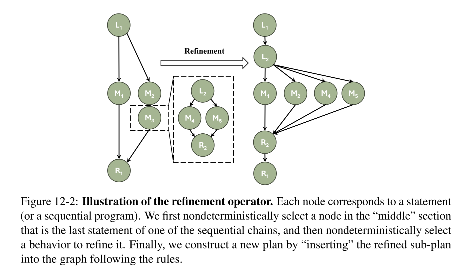
Figure 12-2: Illustration of the refinement operator. Each node corresponds to a statement (or a sequential program). We first nondeterministically select a node in the “middle” section that is the last statement of one of the sequential chains, and then nondeterministically select a behavior to refine it. Finally, we construct a new plan by “inserting” the refined sub-plan into the graph following the rules.
Variable Binding
A bind statement introduces a typed unknown constrained by other variables and state values. The interpreter accumulates these constraints and solves them jointly, often through conditional generators such as motion planners. A candidate plan with free variables is sound only if a satisfying assignment makes its instantiated trace sound. Continuous feasibility remains dependent on the chosen constraint solver and samplers.


Commitment
Commit retains one feasible prefix and its variable assignments, pruning later alternatives like Prolog’s cut. It can dramatically reduce search when subproblems are independent. Incorrect placement can remove the only solution: commitment preserves soundness of a found plan but may sacrifice completeness. Choosing one obstacle placement need not commit the order of all obstacle-removal operations.

The Crow Interpreter
Crow tracks partially ordered left/middle/right programs plus variables and constraints, recursively refining goals and rejecting failed discrete assertions before expensive continuous solving. Iterative deepening makes its depth-first refinement practical. The stated finite-depth completeness claim should be read with the appendix’s idealized exhaustive-refinement/CSP assumptions and the earlier warning about unsafe commits; it is not an unconditional guarantee for arbitrary continuous samplers or erroneous models.
Problem Hardness and Crow Runtime
For discrete planning without bind, regression width K bounds the number of accumulated achieve conditions; the stated search bound is N to an O(K) exponent, with N entities. This motivates iterative widening and serialization of independent goals. Extending the argument to hybrid problems additionally hypothesizes manageable continuous CSP solving; the chapter explicitly warns that difficult sampling constraints can violate that assumption.
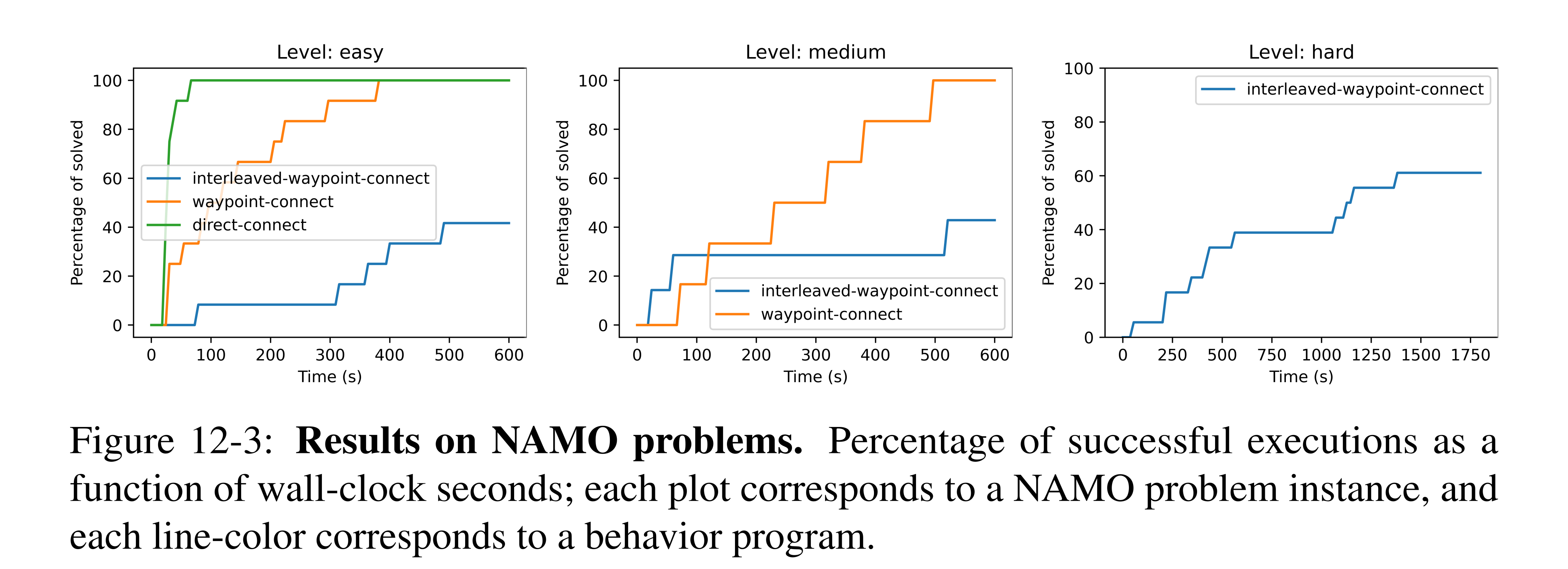
Figure 12-3: Results on NAMO problems. Percentage of successful executions as a function of wall-clock seconds; each plot corresponds to a NAMO problem instance, and each line-color corresponds to a behavior program.
Experiments in NAMO
Three hand-specified NAMO strategies—direct path clearing, waypoint clearing and interleaved waypoint clearing—are run ten times each on three illustrative problem instances. More flexible programs solve harder structures but incur extra branching on easy ones. The evidence demonstrates how one interpreter exploits differing program priors, rather than a broad benchmark against many external planners or a learned strategy-selection system.
Related Work
CDL connects behavior trees, STRIPS, hierarchical task/goal networks, GOLOG-style program search and constraint-based task-and-motion planning. Its distinguishing control is explicit selection of ordering, interleaving and commitments within one program. Representational coverage does not itself establish that every encoding is efficient or complete under aggressive commitments.
Discussion
The proposed next step is to learn and combine transition models, policies, samplers and inference strategies—including ordering and commitments—within CDL. These are opportunities enabled by the representation; the presented experiments use supplied behavior programs and do not demonstrate this integrated learning pipeline.
Epilogue: All You Need is Everything
The proposed full agent would compose problem formulation, perception and reasoning modules. Language models or hand-built rules would formulate states, actions and intentions; modality-specific models would ground them; symbolic search and learned continuous solvers would produce responses. The organizing criterion is effective computation under limits on data, training, memory and inference.
Several essential capabilities remain open. Most presented world models are fixed at test time; the agent must still learn to revise representations, maintain memory, handle partial observability and uncertain dynamics, acquire preferences, preserve skills during continual learning and collaborate with humans. These are proposed future directions rather than demonstrated properties of the component systems.
Encore: Everything is One Thing
The recurring theme is unification: logic with neural computation, planning complexity with circuit complexity, diffusion with constraint satisfaction, language with visual concepts, and policies with declarative models. The examples show why several computational strategies may be useful within one problem.
The author explicitly stops short of a unified theory. Most connections are pairwise, important kinds of reasoning and social understanding are absent, and feasible solutions depend on resource conditions. A general representational or complexity framework is offered as a direction for research, rather than as an established result.
Appendix for Neural Logic Machines
This appendix supplies the original NLM training procedure, task configurations, synthetic data generation, visual-input experiment, acyclic-clause construction, blocks-world example rules, and minimal implementation. It exposes qualifications hidden by the main chapter’s compact performance tables.
Training Method and Curriculum Learning
The decision-task results depend on a staged curriculum, entropy-regularized policy gradients, and balanced reuse of successful and failed instances. These are substantive parts of the learning method.
Training method
Adam uses learning rate 0.005. Supervised batches contain four instances; policy-gradient updates use single episodes with an entropy bonus. Reward is one on success, minus 0.01 per move, with discount 0.99. Sorting trains on sizes four through ten, while path and blocks world reach twelve. Path step limits equal the true shortest distance, explicitly encouraging optimal-length solutions.
Equation

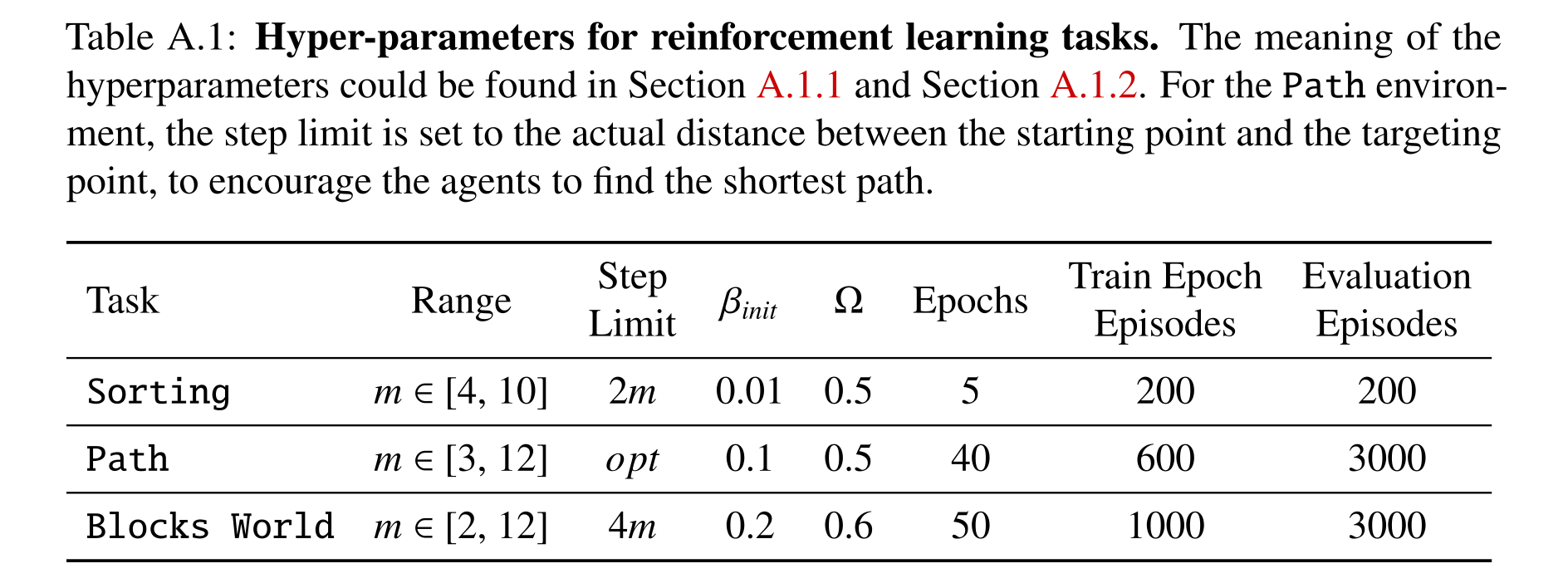
Table A.1: Hyper-parameters for reinforcement learning tasks. The meaning of the hyperparameters could be found in Section A.1.1 and Section A.1.2. For the Path environ- ment, the step limit is set to the actual distance between the starting point and the targeting point, to encourage the agents to find the shortest path.
Curriculum learning guided by exams and fails
Lessons increase object count, with exams drawn from the three latest lesson sizes. Passing thresholds approach 100% at the final lesson, and separate success/failure pools are sampled with probability Ω from successes. The original Algorithm 10 uses a strict greater-than threshold, while the prose defines graduation at 100%; that literal discrepancy remains in the source. The method selects successful graduates and does not ensure every random initialization graduates.
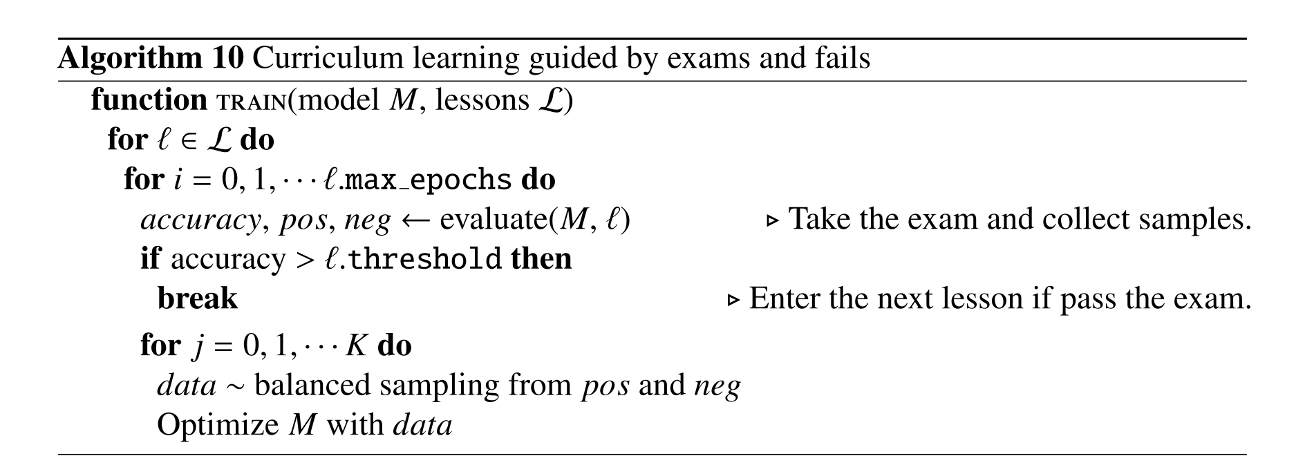
Implementation details and hyper-parameters
The appendix specifies residual predicate access, task capacity, baseline hyperparameters, data generators, the specialized blocks-world head, and how test accuracy is estimated. These details limit claims of learning from minimal structure or uniformly reliable training.
Residual connection.
Residual links concatenate original predicate channels with inferred channels within each arity group. They preserve base facts across layers rather than adding tensors elementwise.
Hyper-parameters for NLM
Reported NLM modules use no hidden perceptron layer and eight intermediate predicate channels. Depth and breadth vary by task. Across ten seeds, graduation is 20% for maternal great uncle, 40% for blocks world, and 60% for path and six-connectivity, despite perfect test accuracy of successful models. Raising maternal-great-uncle training size from twenty to thirty improves graduation to 50%.
Hyper-parameters for MemNN
Memory Networks use the same stated training budgets, key/value widths sixteen and thirty-two, recurrent width sixty-four, and four memory queries except one for sorting. Hyperparameter search reportedly provides little benefit; the comparison remains tied to this input encoding and configuration.
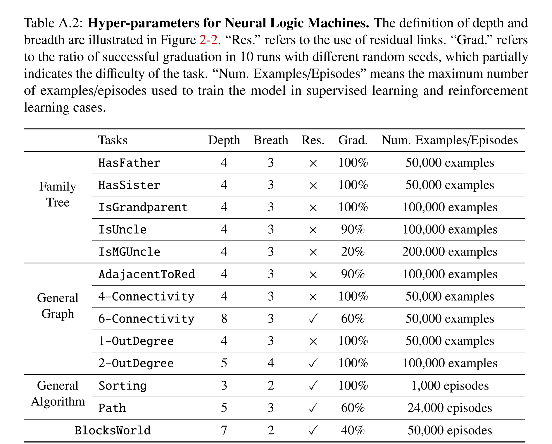
Table A.2: Hyper-parameters for Neural Logic Machines. The definition of depth and breadth are illustrated in Figure 2-2. “Res.” refers to the use of residual links. “Grad.” refers to the ratio of successful graduation in 10 runs with different random seeds, which partially indicates the difficulty of the task. “Num. Examples/Episodes” means the maximum number of examples/episodes used to train the model in supervised learning and reinforcement learning cases.
Data generation
Synthetic families grow through sampled people, parents, and marriages. Graphs place nodes on a unit square and connect sampled numbers of nearest neighbors. Sorting samples permutations; blocks world adds blocks to available supports and shuffles identities. Generalization is measured under these generators, not exhaustive enumeration of all possible relational structures.
Blocks World
Blocks-world training adds supervised cross-entropy prediction of action validity or effects with weight 0.1. The action head manually joins current and target representations for the same object before scoring pairs. These choices supplement the sparse success reward and are important when interpreting claims of learning policies from terminal feedback alone.
Accuracy discussion
Ordinary task results use one thousand sampled test cases. One selected blocks-world model is also tested on one hundred thousand cases without failure; the author reports a 99.7% confidence lower bound of 99.98% accuracy. This is a distribution-specific statistical result for that trained model, not a symbolic correctness proof or a guarantee across seeds.
Neural Logic Machines (NLM) extensions
A jointly trained LeNet replaces node colors with MNIST digit features, and NLM predicts adjacency to a zero. The model trains on one hundred thousand ten-node examples using the MNIST training split and reaches 99.4% on one thousand fifty-node examples. This demonstrates a controlled perception–reasoning composition, rather than general robustness to arbitrary noisy continuous inputs.
Realization of Horn Clause
With sufficient depth, breadth, and channels, a definite clause can be built by expanding body predicates to common arguments, permuting and combining them, reducing body-only variables, and expanding head-only variables. Acyclic rule dependencies can then be topologically ordered and stacked, with disjunction combining multiple rules for one head. The construction concerns representability; unrestricted recursion and guaranteed discovery by gradient descent are outside its scope.
Equations






Sample Blocks World Rules
Nine hand-written helper rules derive clear/moveable blocks, current-world membership, cross-world matches, unmatched blocks below, and ShouldMove. The expanded expression illustrates compositional complexity. These are explanatory rules supplied by the author, not a program extracted from a trained network, and they do not yet choose the destination of a move.
Equations
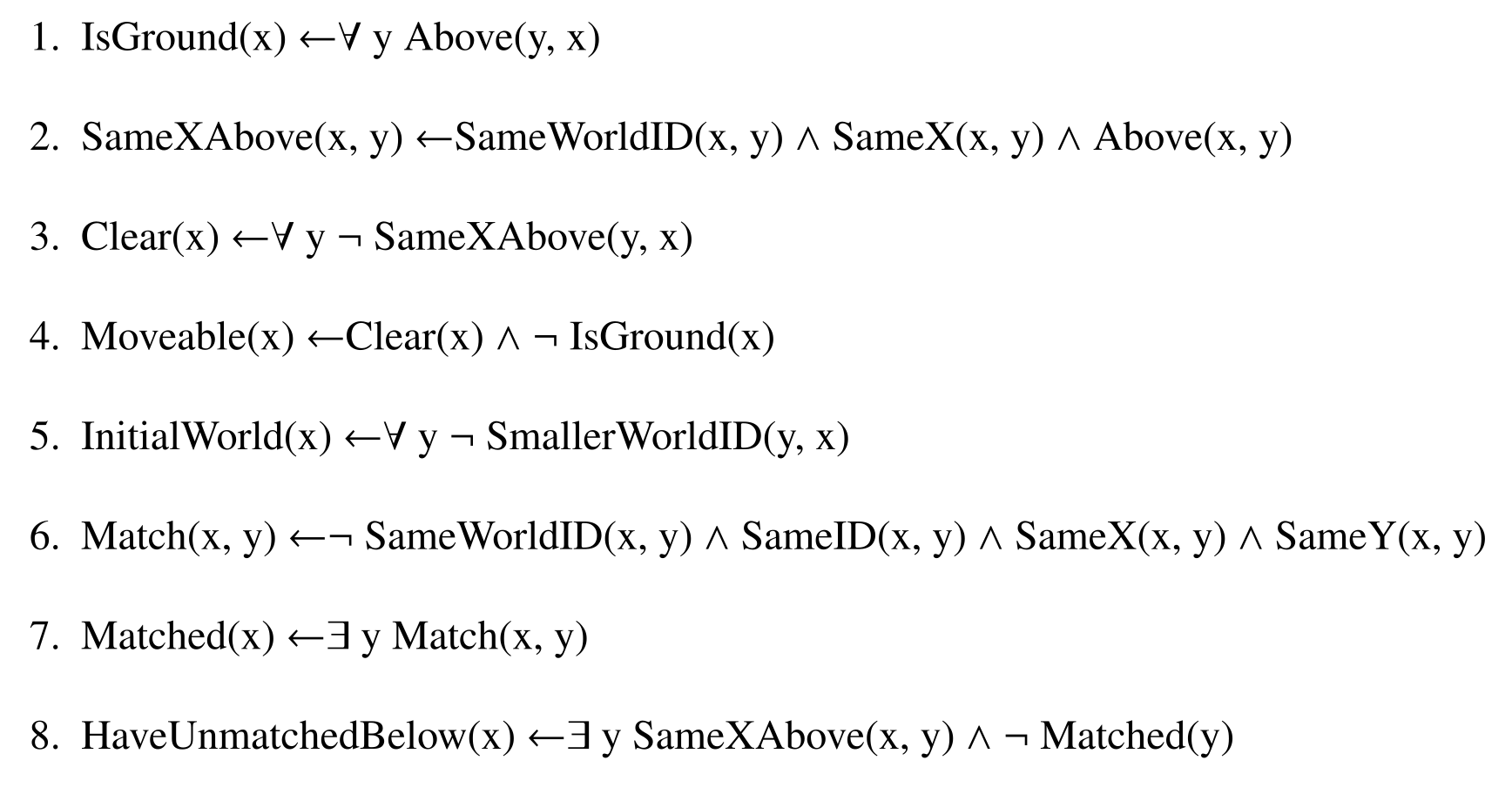


Implement NLM in TensorFlow
The fifty-nine-line TensorFlow example implements one breadth-three layer, including broadcast expansion, masked maximum/minimum reductions, tuple permutations, shared sigmoid transformations, and concatenated residual inputs. Diagonal masks exclude repeated-object tuples. It is a minimal historical layer implementation, not the complete training system; its source spelling and indentation are part of the original code.
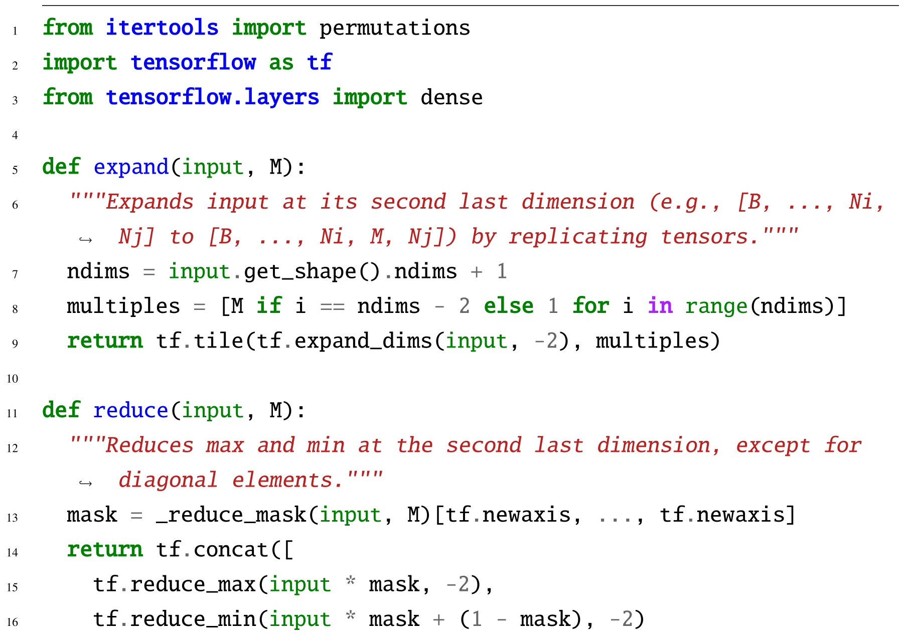
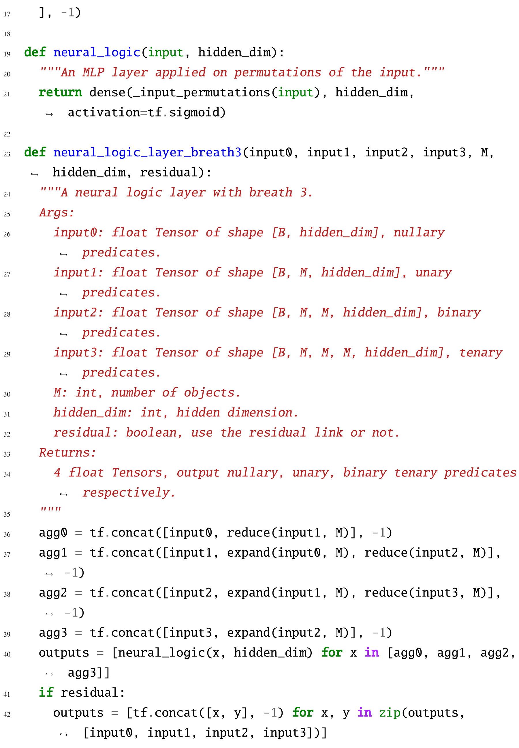
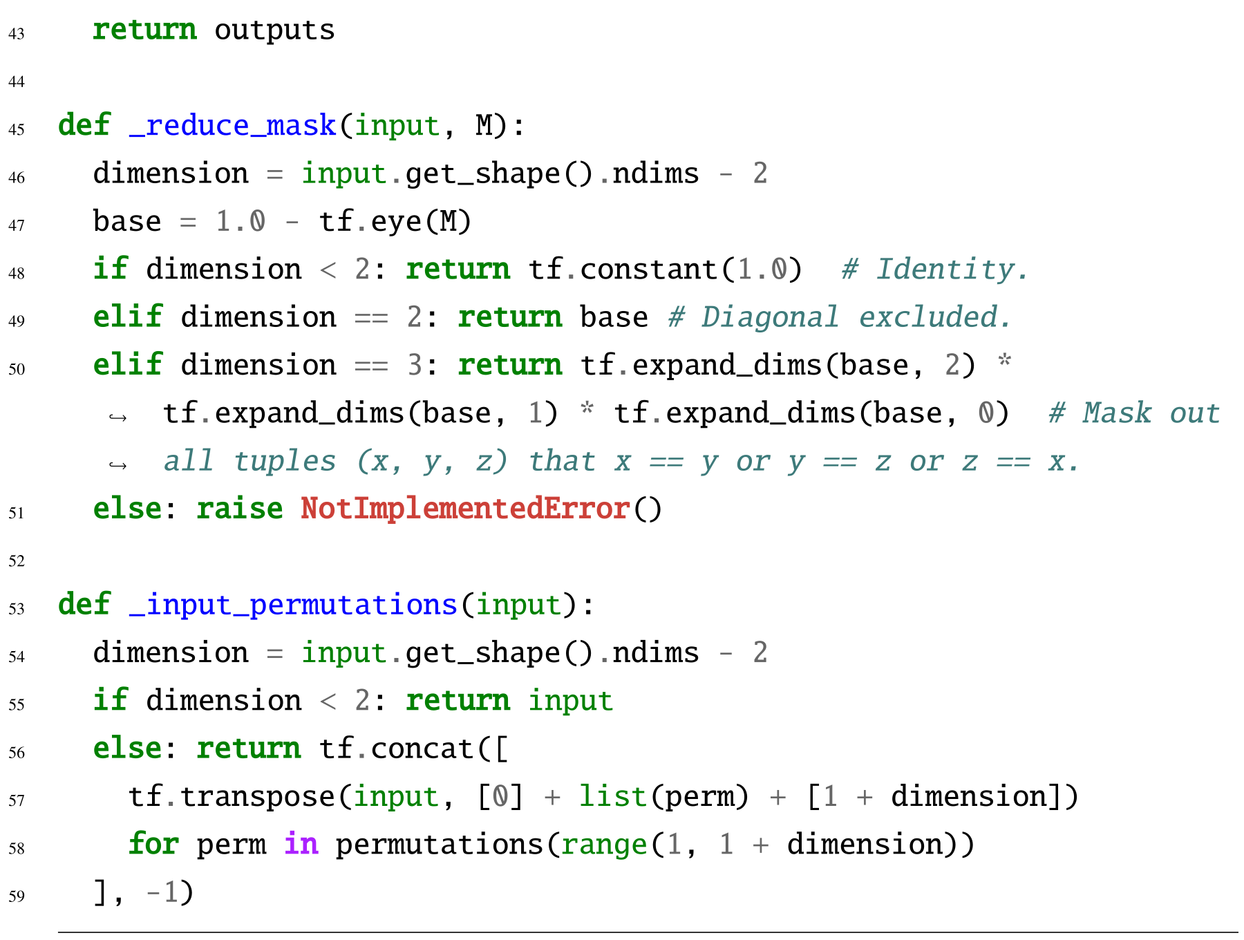
Appendix for Sparse and Local Neural Logic Machines
The SpaLoc supplement documents architecture and sampling settings, three-seed errors, sparsity and arity ablations, information-based label calibration, path counting, and the exact synthetic family relations. These details help separate the sources of efficiency and accuracy.
Experimental configuration
SpaLoc uses Adam at 0.005, breadth three, no hidden layer in its predicate transforms, sigmoid activations, sparsity weight 0.01, and inference gate threshold 0.05. The threshold was chosen using validation accuracy; values from 0.01 to 0.1 reportedly have little effect. Family subgraphs contain twenty nodes, while knowledge-graph configurations use ten or twenty, with task-specific batch sizes, depths, feature widths, and path-count cutoffs.
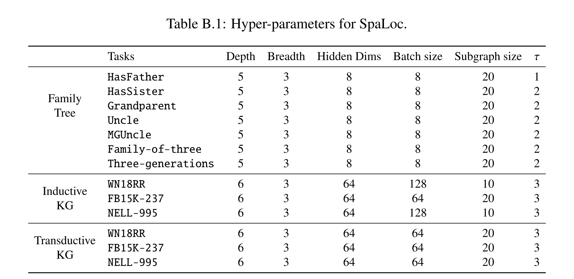
Table B.1: Hyper-parameters for SpaLoc.
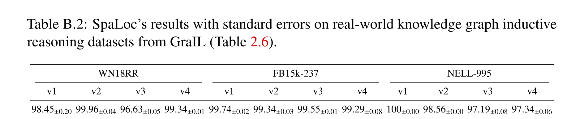
Table B.2: SpaLoc’s results with standard errors on real-world knowledge graph inductive reasoning datasets from GraIL (Table 2.6).
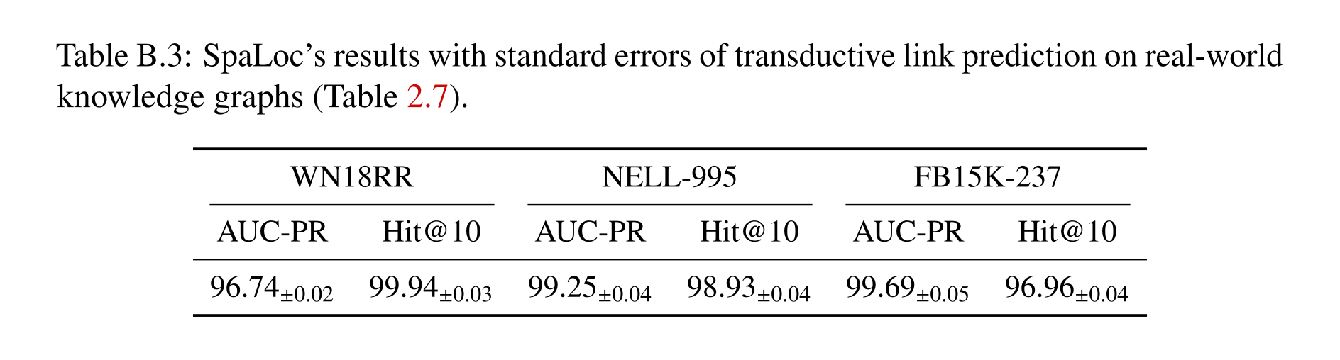
Table B.3: SpaLoc’s results with standard errors of transductive link prediction on real-world knowledge graphs (Table 2.7).
SpaLoc's results with standard errors
Tables B.2 and B.3 report standard errors over three random seeds for the inductive and transductive knowledge-graph results. Small reported errors indicate consistency in this evaluation protocol; they do not address the full-negative-ranking failure discussed in the main chapter.
Implementation of subgraph samplers
Sampling first projects a hypergraph to a binary graph by connecting nodes that share any hyperedge. Neighbor expansion or path sampling selects nodes in this projection, then the method induces the original hypergraph on that node set. The projection guides locality while the induced graph retains original higher-arity relations.
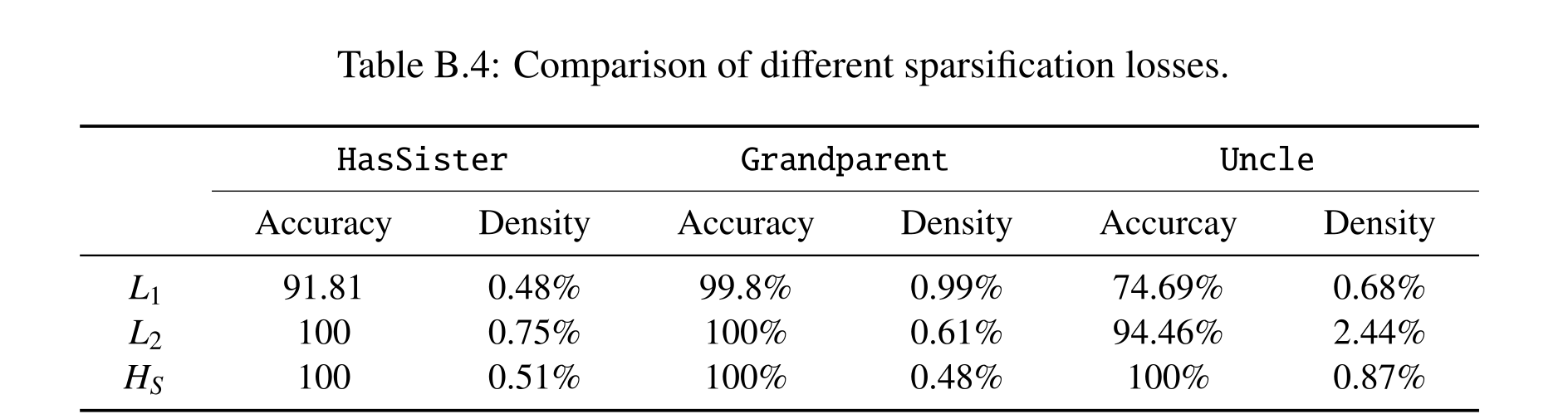
Table B.4: Comparison of different sparsification losses.
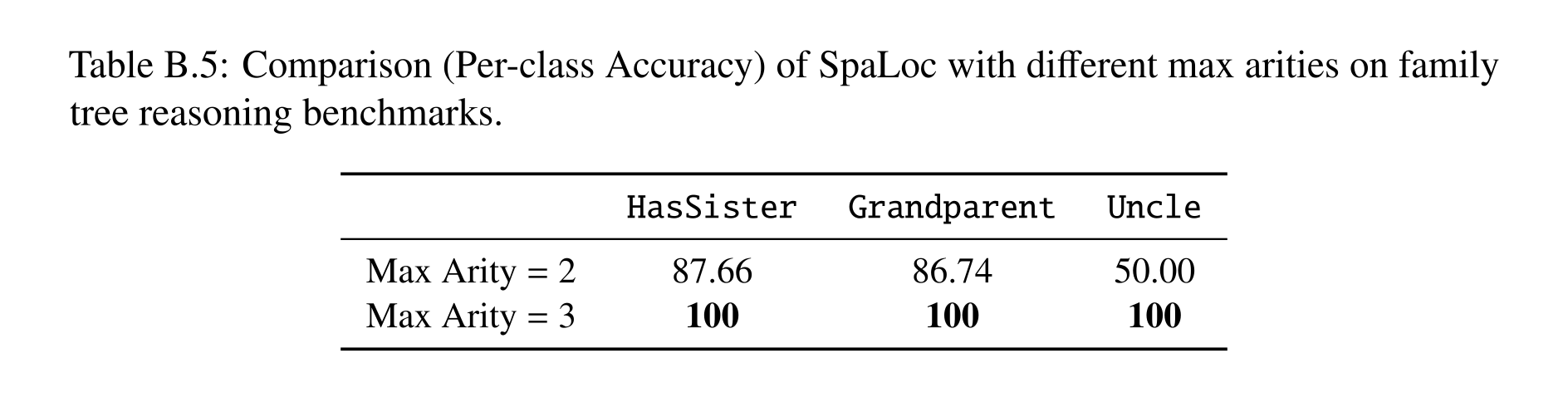
Table B.5: Comparison (Per-class Accuracy) of SpaLoc with different max arities on family tree reasoning benchmarks.
Ablation study on sparsification loss
On hundred-object family tests, Hoyer-Square achieves 100% on the three reported relations while keeping intermediate nonzero density below one percent. L1 is sometimes sparser but less accurate, and L2 also loses accuracy on Uncle. The result supports an accuracy–density tradeoff for these tasks rather than universal dominance in sparsity alone.
Ablation study on SpaLoc's maximum arity
Reducing maximum arity from three to two substantially hurts the family relations despite binary inputs and outputs; Uncle drops from 100% to 50%. Ternary representations also improve the three reported knowledge-graph subsets. The ablation supports higher-order intermediate reasoning in this model family, without establishing that every possible architecture needs the same arity.
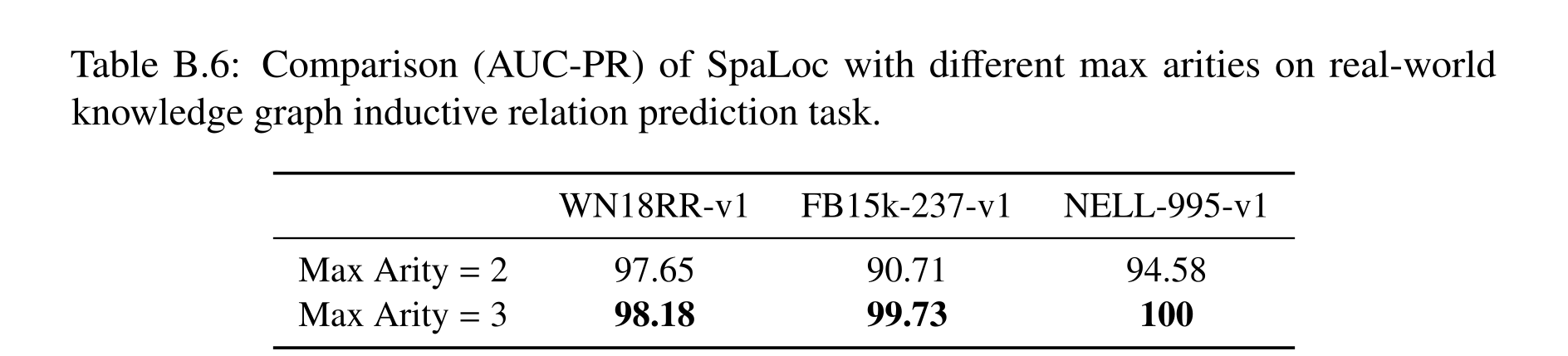
Table B.6: Comparison (AUC-PR) of SpaLoc with different max arities on real-world knowledge graph inductive relation prediction task.
Ablation Study on Label Adjustment
Information-sufficiency adjustment is compared with unchanged labels and constant 0.9 scaling of positive labels. Its combination with neighbor sampling performs best in the reported HasFather and HasSister tests. Poor random-node sampling still leaves HasFather at chance even with adjustment, showing that calibration cannot fully replace useful evidence selection.
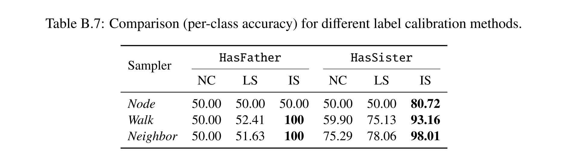
Table B.7: Comparison (per-class accuracy) for different label calibration methods.
Calculation of the information sufficiency
The computation uses a vertex–hyperedge incidence matrix and powers of its induced connectivity matrix to count bounded-hop connections. For binary target pairs it combines the higher-hop incidence matrix with the incidence transpose; unary queries sum incident counts. Matrix powers count walks with multiplicity, so this is a tractable connectivity-based sufficiency statistic rather than enumeration of distinct simple proofs of a target relation.
Definition of Relations in Family Tree
The benchmark supplies Father, Mother, Son, and Daughter and defines five unary/binary targets plus the ternary Family-of-three and Three-generations relations. The original formulas specify argument direction and exclusions and should govern interpretation of the relation names. Families are procedurally generated, then labeled from these definitions; the experiment is supervised relational induction with known synthetic labeling rules.
Equation
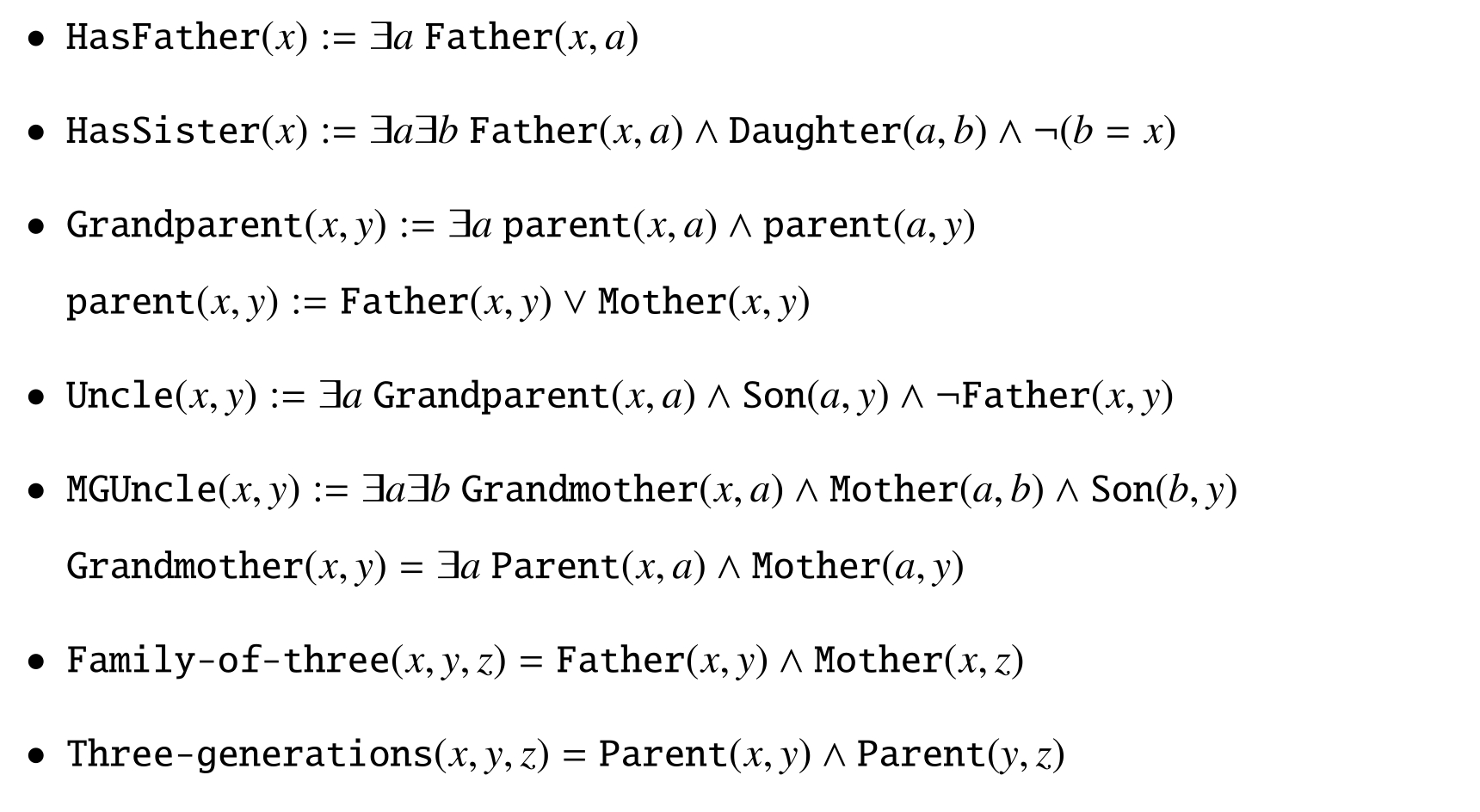
Appendix for Temporal and Object Quantification Networks
Appendix C specifies TOQ-Net and comparison architectures, feature preprocessing, capacity variants, and optimization. Its architecture tables and binary-input ablations are needed to interpret the main experiments.
Implementation Details
The appendix details five baseline families plus a binary-input STGCN extension. Soccer training balances action categories and trajectories; manipulation experiments use raw object states. Main-text and appendix descriptions differ on temporal depth, so the retained specifications should not be treated as a single unambiguous configuration.
TOQ-Nets
The appendix specifies three relational and three temporal layers, with channel sizes 16/48 for soccer and 48/144 for manipulation; the main text instead selects four temporal layers. Soccer preprocessing computes ground/vertical speeds, acceleration, and pairwise distances, normalizes them, and learns five sigmoid threshold features per quantity while annealing the temperature from 1 to 0.001. Thus useful physical quantities are designed even though thresholds and higher-level predicates are learned. Manipulation uses a 64-channel affine-sigmoid feature extractor.
Equation

STGCN
STGCN applies graph propagation and temporal convolutions, pools entity/time axes, and classifies the resulting feature vector. Soccer inputs omit pairwise distances because the original architecture accepts unary features; manipulation uses the same object-state inputs as TOQ-Net. Table C.4 retains full, small, and tiny architectures for the capacity comparison.
STGCN-MAX
STGCN-MAX replaces averaged neighbor messages with featurewise maxima, bringing spatial aggregation closer to relational quantification while retaining temporal convolutions. It tests whether max aggregation alone explains the benefit.
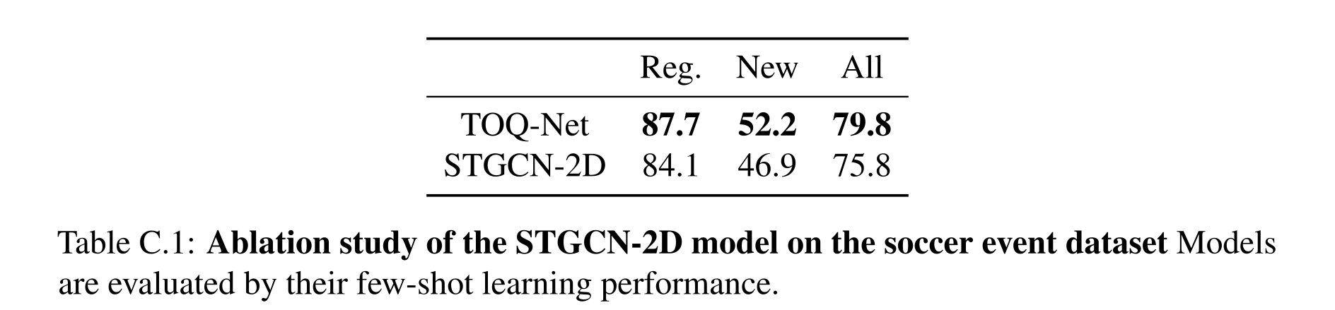
Table C.1: Ablation study of the STGCN-2D model on the soccer event dataset Models are evaluated by their few-shot learning performance.
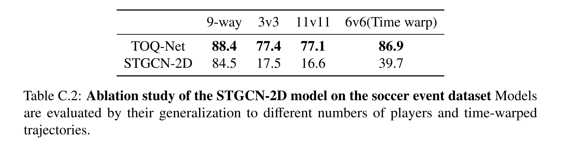
Table C.2: Ablation study of the STGCN-2D model on the soccer event dataset Models are evaluated by their generalization to different numbers of players and time-warped trajectories.
STGCN-2D
STGCN-2D adds binary distance inputs, improving soccer few-shot accuracy to 46.9% and overall accuracy to 75.8%. It still generalizes poorly from 6v6 to 3v3/11v11 (17.5%/16.6%) and to time-warped 6v6 (39.7%), versus 77.4%/77.1%/86.9% for TOQ-Net. Pairwise inputs therefore close part of the ordinary-classification gap without reproducing the structural transfer.
STGCN-LSTM
STGCN-LSTM pools entity features at each time and feeds a two-layer bidirectional LSTM. Temporal convolution uses kernel three for soccer and kernel one for manipulation to isolate recurrent temporal modeling. The RLBench ablation finds similar one-shot performance for kernels one and three (95.48% and 96.16%), both below TOQ-Net’s 98.04%.
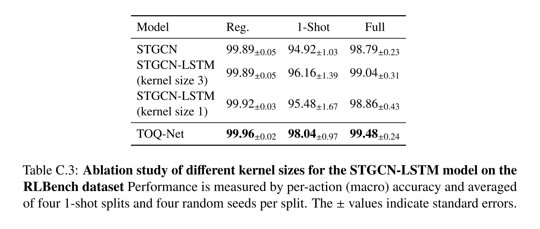
Table C.3: Ablation study of different kernel sizes for the STGCN-LSTM model on the RLBench dataset Performance is measured by per-action (macro) accuracy and averaged of four 1-shot splits and four random seeds per split. The ± values indicate standard errors.
Space-Time Region Graph Networks
Space-Time Region Graph Networks propagate information over a graph containing entities across frames. Table C.5 specifies full, small, and tiny variants; the model provides a comparison to graph-based spatiotemporal aggregation without TOQ-Net’s explicit ordered interval operations.
Non-Local Neural Networks
Non-local networks replace graph convolution on the space-time graph with attention across nodes; Table C.6 lists capacity variants. Soccer training uses balanced batches of 128, Adam at 0.002, 200 epochs, and validation-triggered decay after the first 50 epochs; scale-transfer models receive 10,000 finetuning iterations. Manipulation uses Adam at 0.003 for 150 epochs, with batch size 32 for STGCN backbones and four for TOQ-Net. These differing batch sizes are part of the stated protocol.
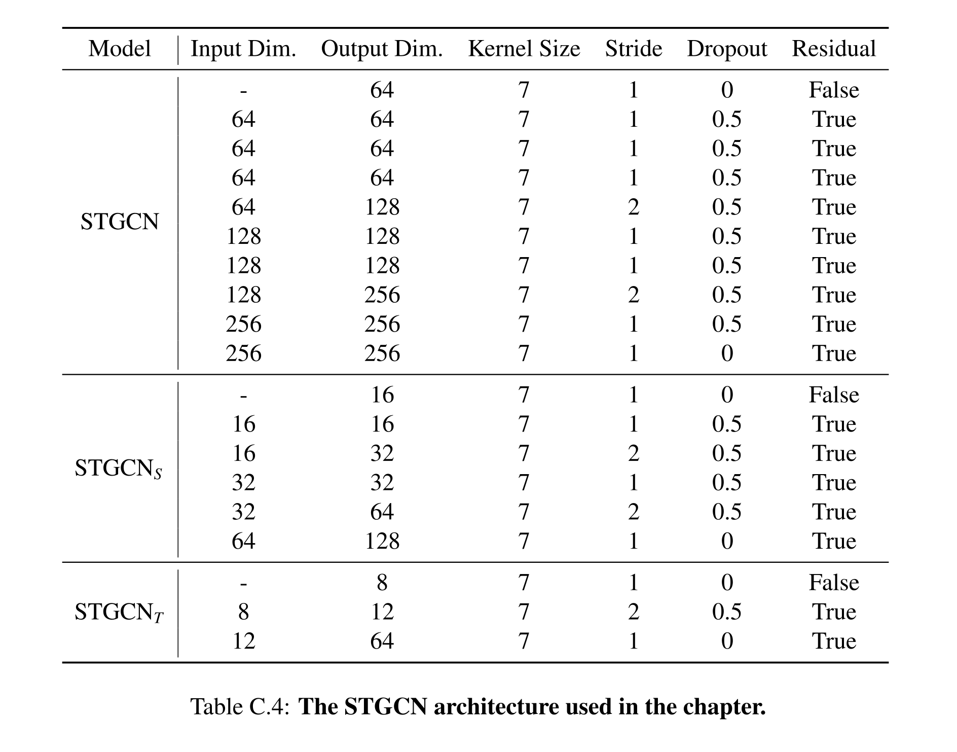
Table C.4: The STGCN architecture used in the chapter.
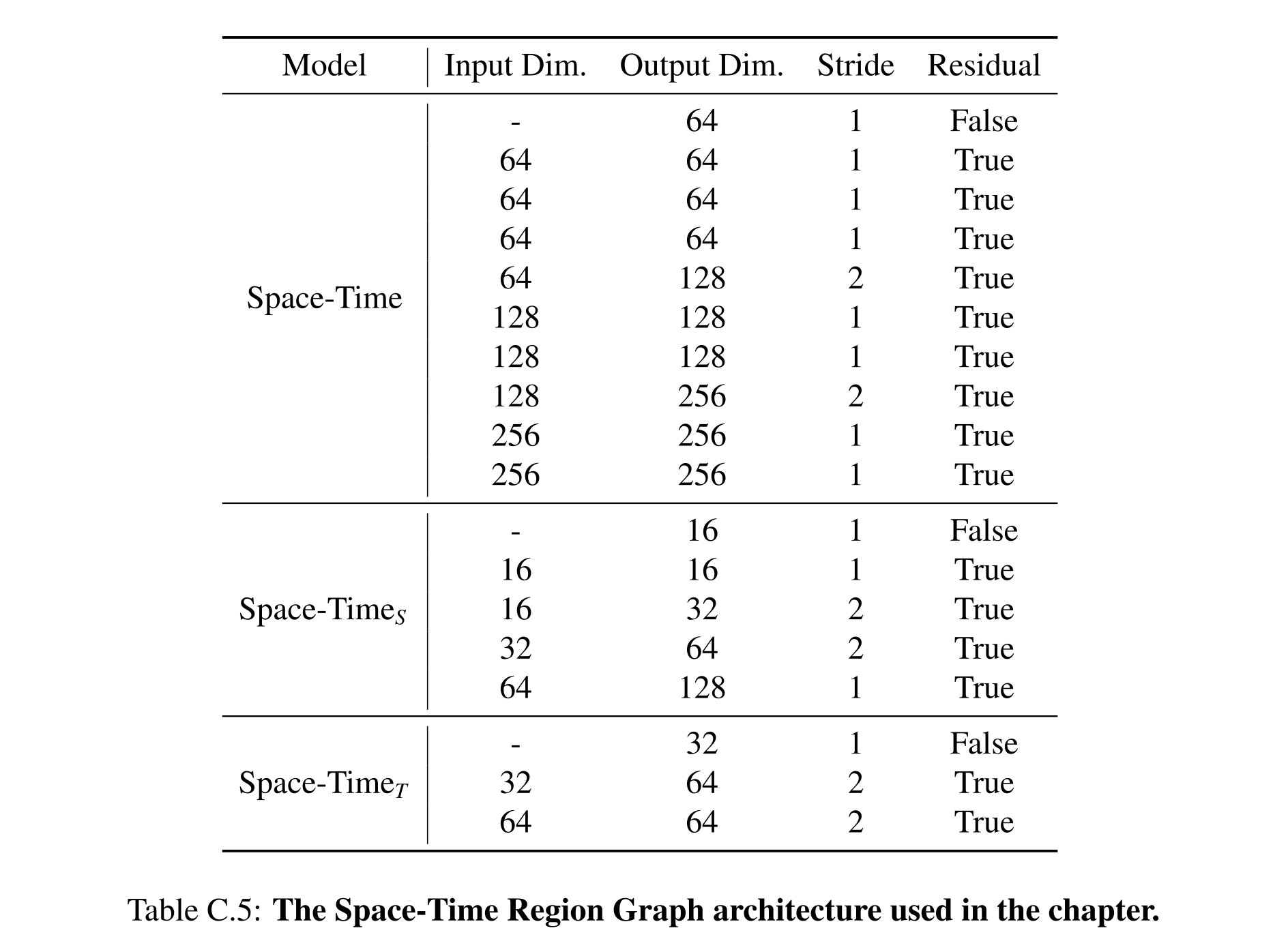
Table C.5: The Space-Time Region Graph architecture used in the chapter.
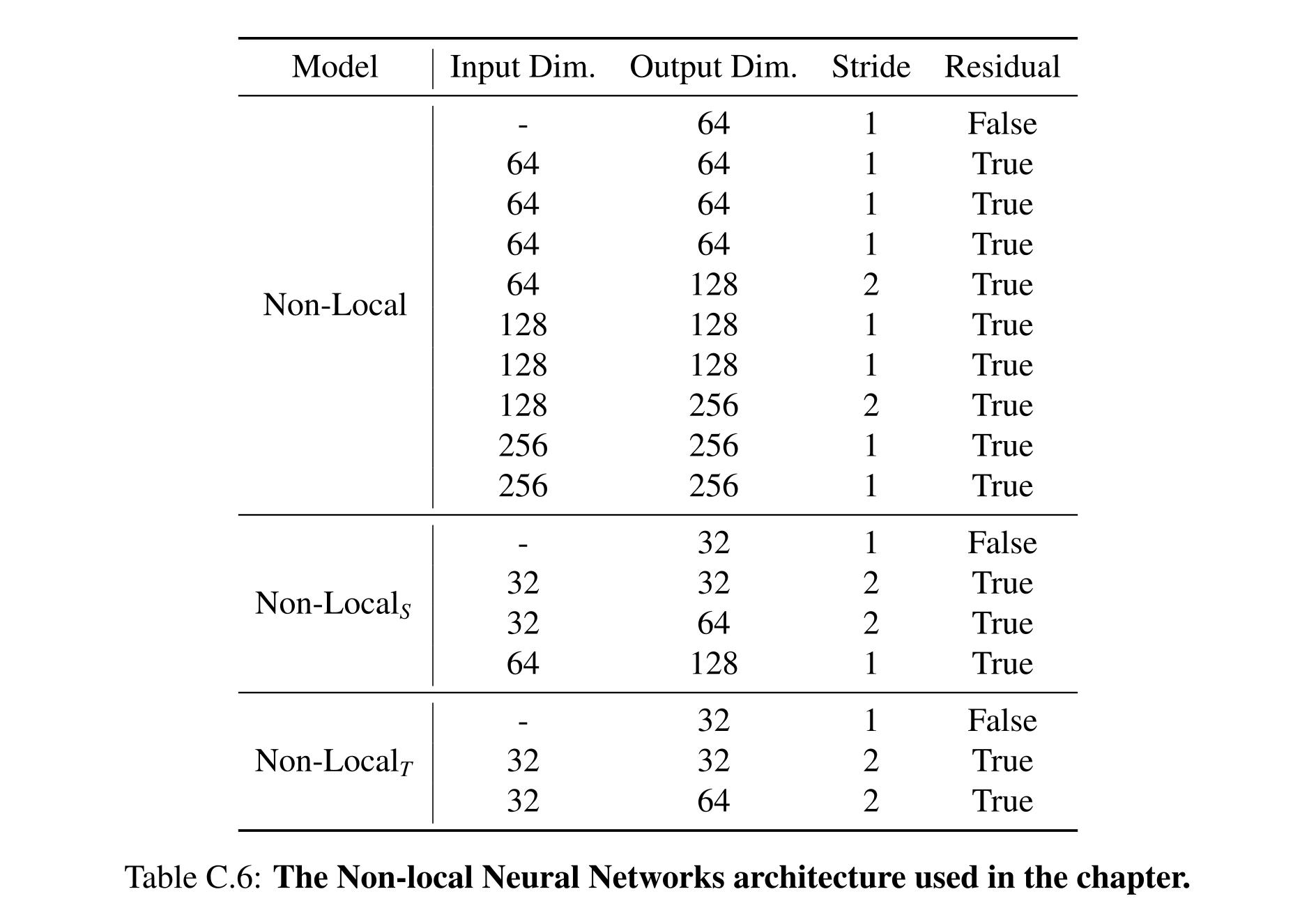
Table C.6: The Non-local Neural Networks architecture used in the chapter.
Appendix for Expressivity of Neuro-Symbolic Logic Models
Appendix D supplies search and circuit constructions, domain-specific width analyses, and experimental generation/training details. The proofs rely on the definitions of serializability and SOS; the supplementary examples also show why ordinary narrow rules alone are insufficient.
Proofs and Discussions for Search Complexity
The search analysis distinguishes a general exhaustive variant from the simplified efficient algorithm. It proves optimality for the serializable class, explains the added SOS condition needed for the width bound, and connects regression constraints with forward tuple novelty.
Complete and Optimal Version of S-GRS
The general version tracks multiple resulting trajectories/states for each serialized subgoal, including empty subtrajectories when a prior step already establishes the next condition. Loop-free trajectories ensure termination. This recovers the stated completeness/optimality but may be slower than plain backward search: the source gives O(3N) versus O(2N) state/constraint combinations. Retaining only one subgoal outcome is therefore a consequential restriction.
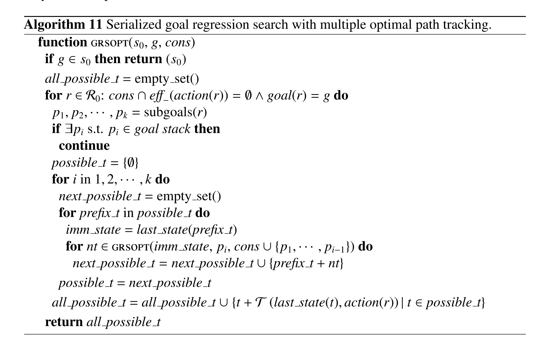
Proof for Theorem 4.3.1: S-GRS Optimality and Completeness
The optimality proof inducts on the returned plan distance. Zero-distance goals are already satisfied; for a serializable rule, optimal recursive subplans concatenate into an optimal prefix and finally an optimal goal plan. Completeness is asserted for the defined set of goals solvable through such rules, so the theorem does not cover an arbitrary planning instance.
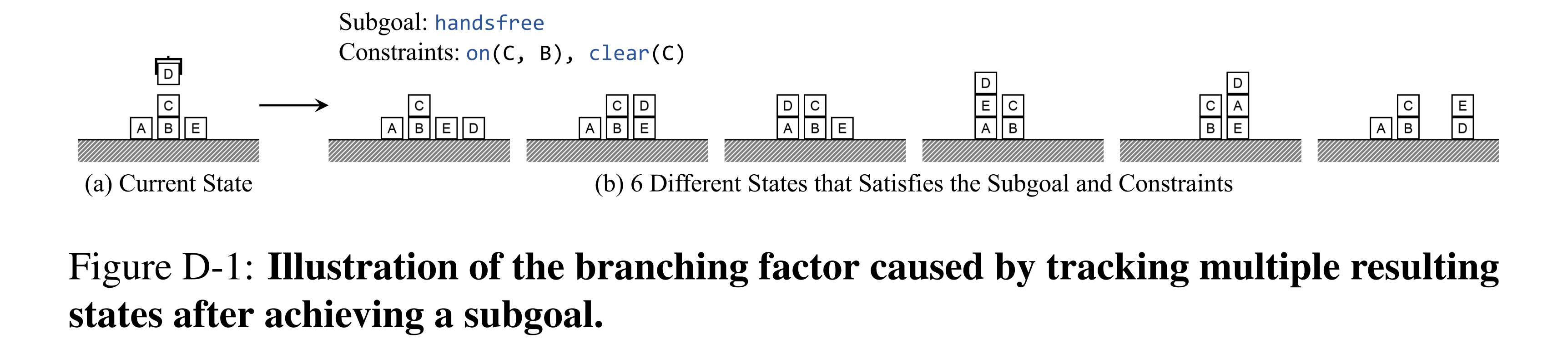
Figure D-1: Illustration of the branching factor caused by tracking multiple resulting states after achieving a subgoal.
Making Non-SOS Problem Serializable
Nonserializable preconditions can be bundled into a new conjunctive “super predicate,” with actions split to maintain its truth. This makes interactions explicit but can expand predicates and operator variants exponentially. The source’s illustrative operator update contains notation slips; its intended tradeoff is the added representation cost, not a ready-to-run action specification.
Proof for Theorem 4.3.2: Polynomial Hardness for SOS-k problems.
The stated polynomial bound counts O(Nk+1) goal/constraint combinations and invokes SOS to justify reusing one optimal representative. Candidate bounded-width rules can be enumerated without prior access to the successful rule set. Without SOS, free-variable choices and different intermediate states can invalidate cached continuations even for width-zero rules, so narrow syntax alone does not imply the theorem’s complexity bound.
Additional Discussion
Lifted domain analysis can reject regression orders that require the goal itself or violate maintained facts, though serializability remains state-dependent and difficult in general. Constraint width resembles the backward dependencies counted in constraint-graph treewidth; delete relaxation instead exploits a kind of parallel achievement. Universal preconditions create unbounded subgoal lists, potentially factorial order search and growing constraints unless additional selector structure is supplied.
Connection with Width-Based Forward Search IW(k)
The forward-width proof argues that every action on an optimal SOS-width-k trajectory achieves a novel tuple of at most k+1 atoms; otherwise the plan could be shortened. This makes the goal reachable in IW(k+1)’s tuple graph. The bound is one-way: clearing a block can have SOS width one yet forward width one, rather than the upper bound two.
Equation

Proofs and Discussions for Policy Circuit Complexity
Policy compilation translates lifted logical update rules into relational layers. The resulting bounds concern existence of circuits and the state/goal information they must track; the appendix also discusses recurrent computation and domain shortcuts as ways to reduce repeated regression.
Proof of Theorem 4.4.1: Compilation of BWD
The BWD construction stores which conjunctive subgoals regress to the target in each number of steps. A layer applies all relevant action regressions, and a satisfaction check against the current state identifies an executable first action. Conjunctions involving at most kBWD atoms require at most βkBWD object variables, giving the stated breadth and O(T) depth bound.
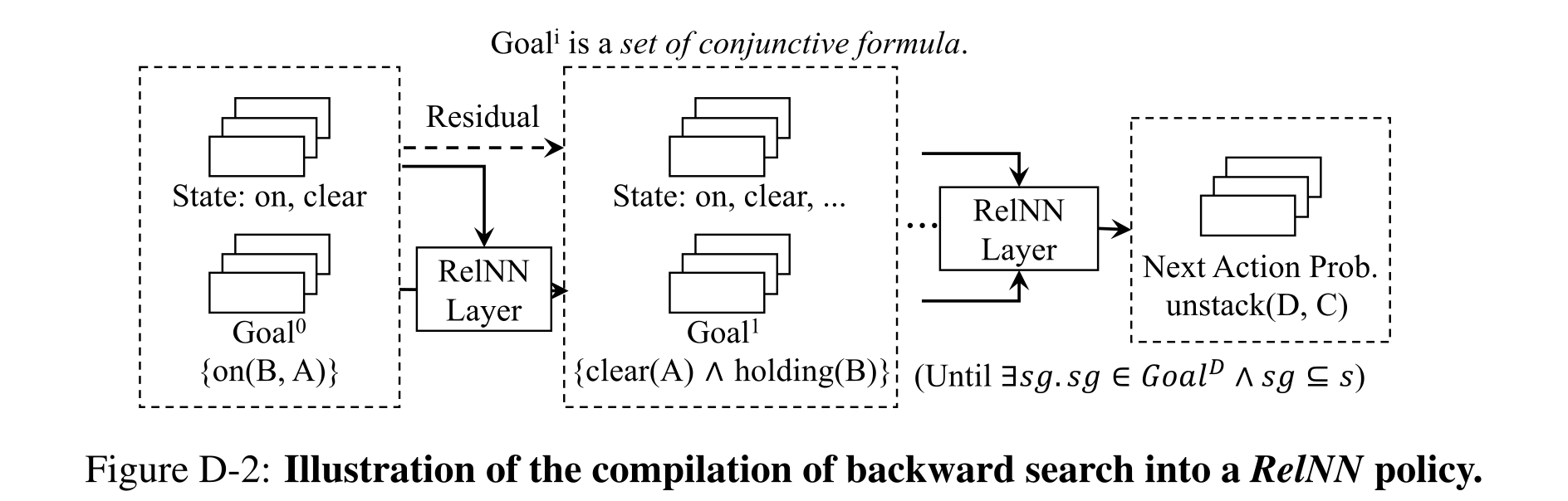
Figure D-2: Illustration of the compilation of backward search into a RelNN policy.
Proof of Theorem 4.4.2: Compilation of S-GRS
The appendix implements the SOS result through IW(k+1): track bounded atom tuples reachable within each depth and the representative successor-state information associated with them, then extend via grounded actions. It argues that replanning from the selected next state follows a compatible tuple path. Direct compilation of S-GRS is described as possible but omitted; the presented proof is a representability construction, not released executable compiler code.
More Discussion
A parameter-shared layer can be iterated a number of times that grows with the instance. Alternatively, a new predicate can expose an expensive relation: given above(x,y), the top clear block above a target is locally selectable. Such a shortcut changes the available representation; computing that relation from immediate on-relations still requires work. The maze example similarly uses a domain-specific traversal/linearization idea rather than a general fixed-depth planning result.
Analysis of AI Planning Problems
The six-domain classification assumes a single-atom goal and the stated action models. Gripper has constant depth because every room is directly reachable; other constant-breadth examples can require paths or tower traversal. Optimal conjunctive goals need not serialize, while satisficing goals in Logistics, Gripper, Rover, and Elevator can be handled one at a time. Super predicates can restore serialization at substantial representation cost.
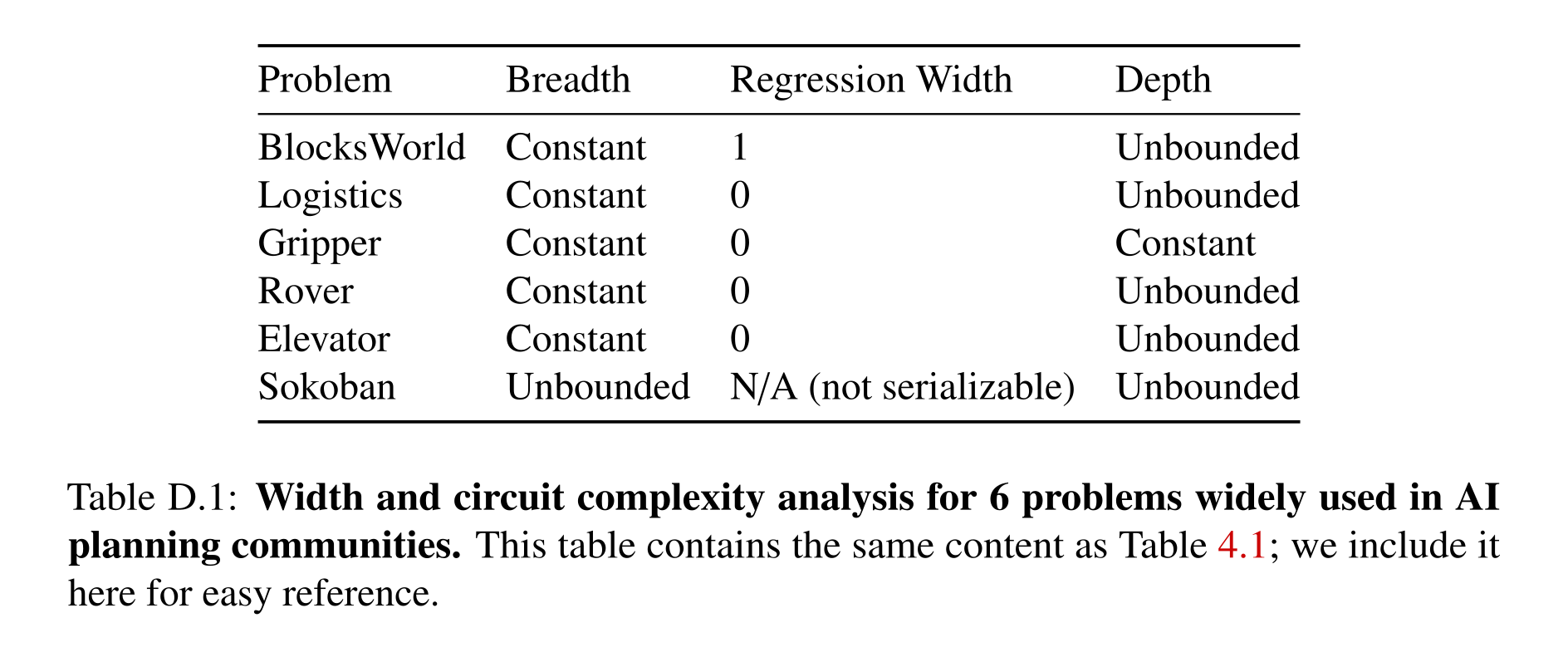
Table D.1: Width and circuit complexity analysis for 6 problems widely used in AI planning communities. This table contains the same content as Table 4.1; we include it here for easy reference.
SOS Width Analysis
Explicit BlocksWorld and Logistics regression schemas illustrate bounded constraint width. BlocksWorld follows the object currently blocking a target and maintains the necessary clear condition while freeing the hand; Logistics decomposes delivery through loading, vehicle movement, and unloading. The original formulas omit static type constraints and contain variable/name inconsistencies, so they are retained as analytical sketches rather than a verified executable domain.
Equations
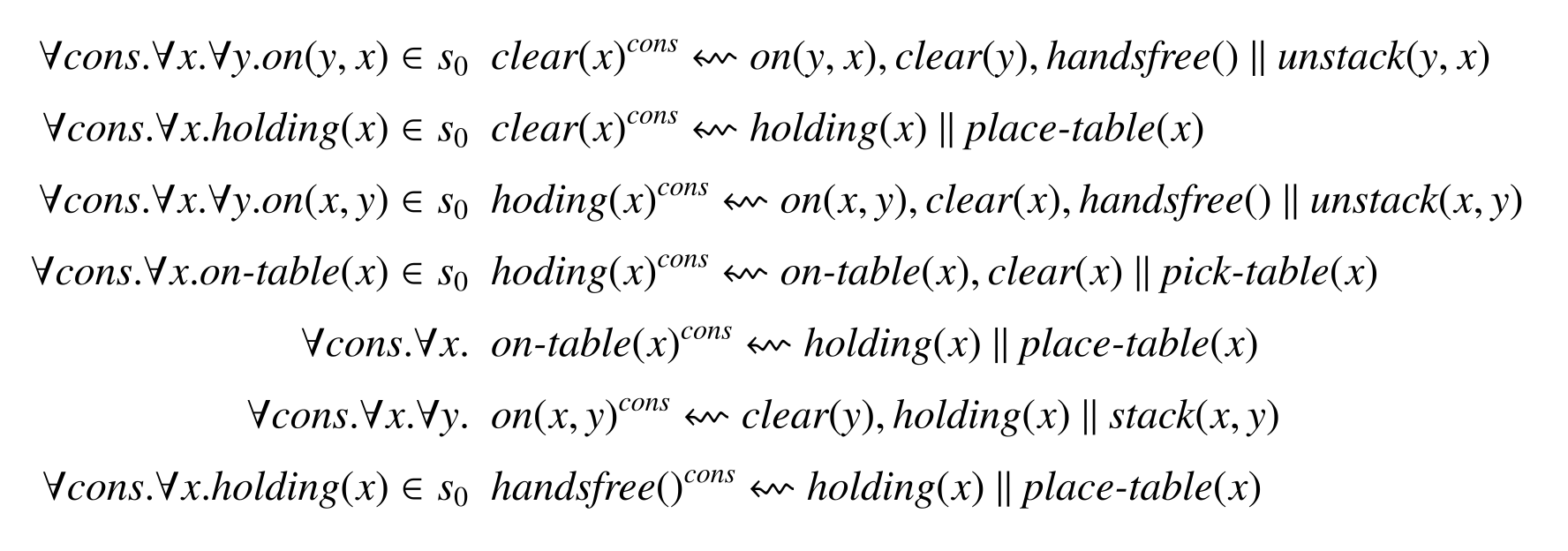
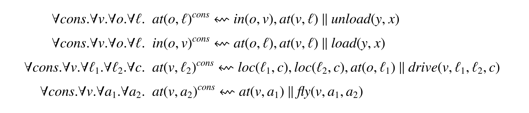
Experimental Details
Experimental details specify the deliberately structured instance generators and common optimizer settings used to probe depth and breadth. They are essential context for the perfect generalization scores in the main table.
Training details
Assembly3 generates exactly one compatible A/B/C triple. BlocksWorld samples piles incrementally and targets an initially covered block. Logistics begins with a directed tree and adds a few forward edges, producing graphs that usually lack mutual reachability between start and goal. Models use Adam at 0.001 with standard moment coefficients and one Titan RTX per experiment; the main text specifies 64 hidden channels and task-dependent depth. The released goal-regression-width repository supplies the experimental implementation.
Appendix for Diffusion Continuous Constraint Satisfaction Solver
Appendix E details synthetic data and state encodings, model composition, sampling costs, failure cases, and integration with task search. Original visualizations show both successful and invalid samples and all learned qualitative gradient fields.
Problem Domains and Data Generation
Datasets balance examples across the included object counts and derive feasible configurations from geometric construction plus simulation/planning checks. The input representations deliberately simplify shapes and pose freedoms; these choices bound what the experiments establish.
2D Triangle Packing
Triangle data uses Bowyer–Watson triangulation of random tray points followed by slight shrinking. Geometry is represented in a canonical resting orientation by one edge length and a remaining vertex vector; pose contains a 2D vertex location and sine/cosine rotation. This constructs densely packed feasible training configurations without solving arbitrary initial packing problems.
2D Shape Arrangement with Qualitative Constraints
Rectangle data recursively partitions a tray to depth three, adds padding, and removes very small regions. Eleven qualitative relations are labeled by explicit rules, such as a distance threshold relative to object widths for close-to. Geometry uses width/length; pose uses centroid and sine/cosine yaw, allowing vertical placements when required.
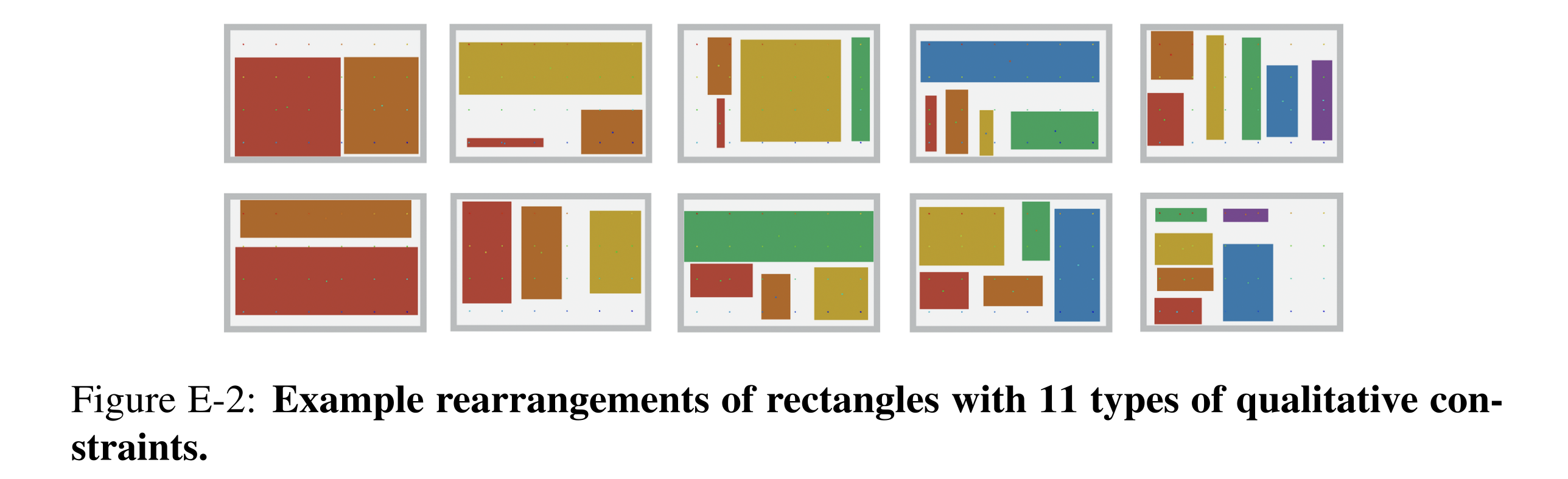
Figure E-2: Example rearrangements of rectangles with 11 types of qualitative con- straints.
3D Object Stacking with Stability Constraints
Stacking data partitions a vertical region into shapes, lets them settle in PyBullet, checks final stability, and removes objects sequentially to verify intermediate configurations. An upper shelf limits free space. Geometry and pose are represented in a planar cross-section with roll, even though stability is tested in a 3D simulator; the benchmark does not cover unrestricted spatial orientations.
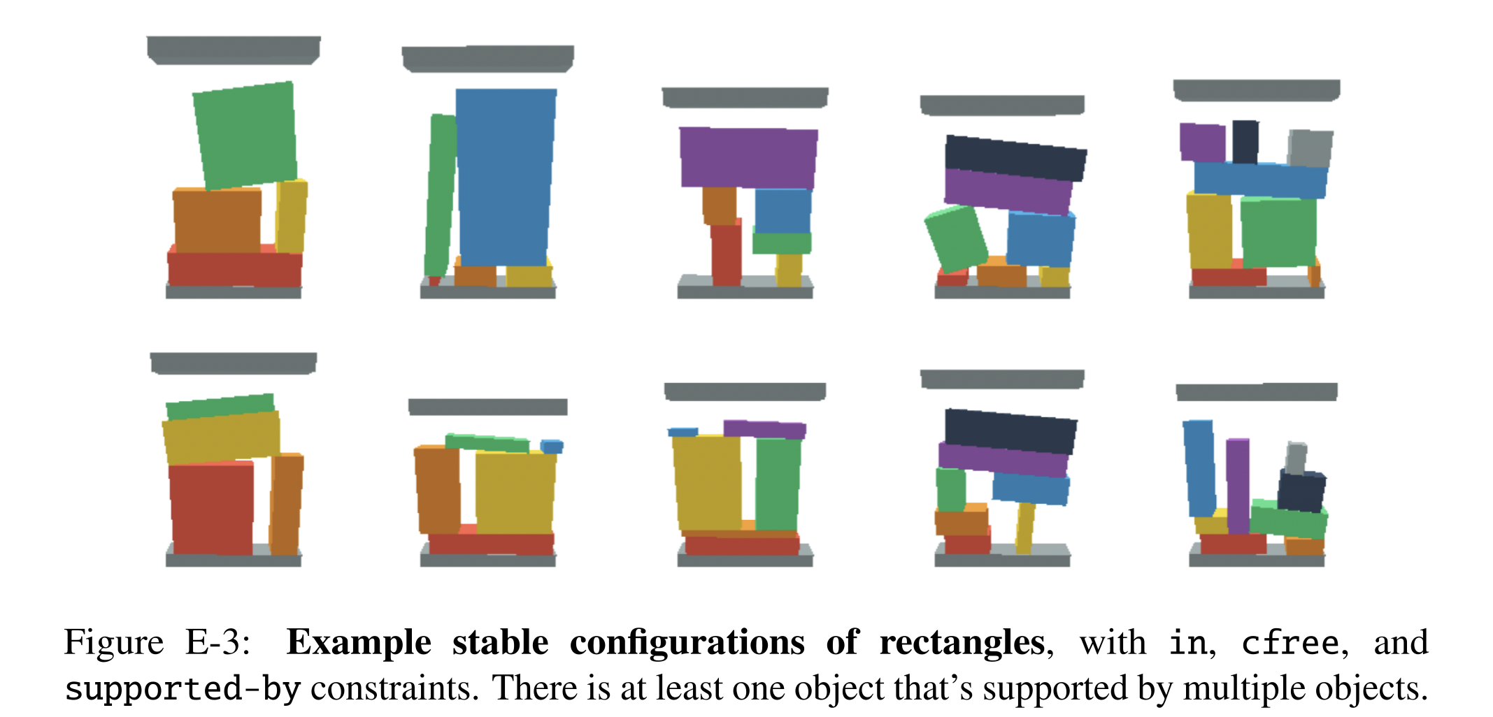
Figure E-3: Example stable configurations of rectangles, with in, cfree, and supported-by constraints. There is at least one object that’s supported by multiple objects.
3D Robot Packing with Robots
Robot data comprises ten categories and 53 assets, with precomputed grasps directed at five object faces. Tray partitions determine candidate object sizes/placements, then a planner checks placement orders, grasp combinations, gripper collisions, and arm trajectories. Bounding boxes encode geometry, a five-way vector encodes grasp direction, and translation plus yaw encodes placement.
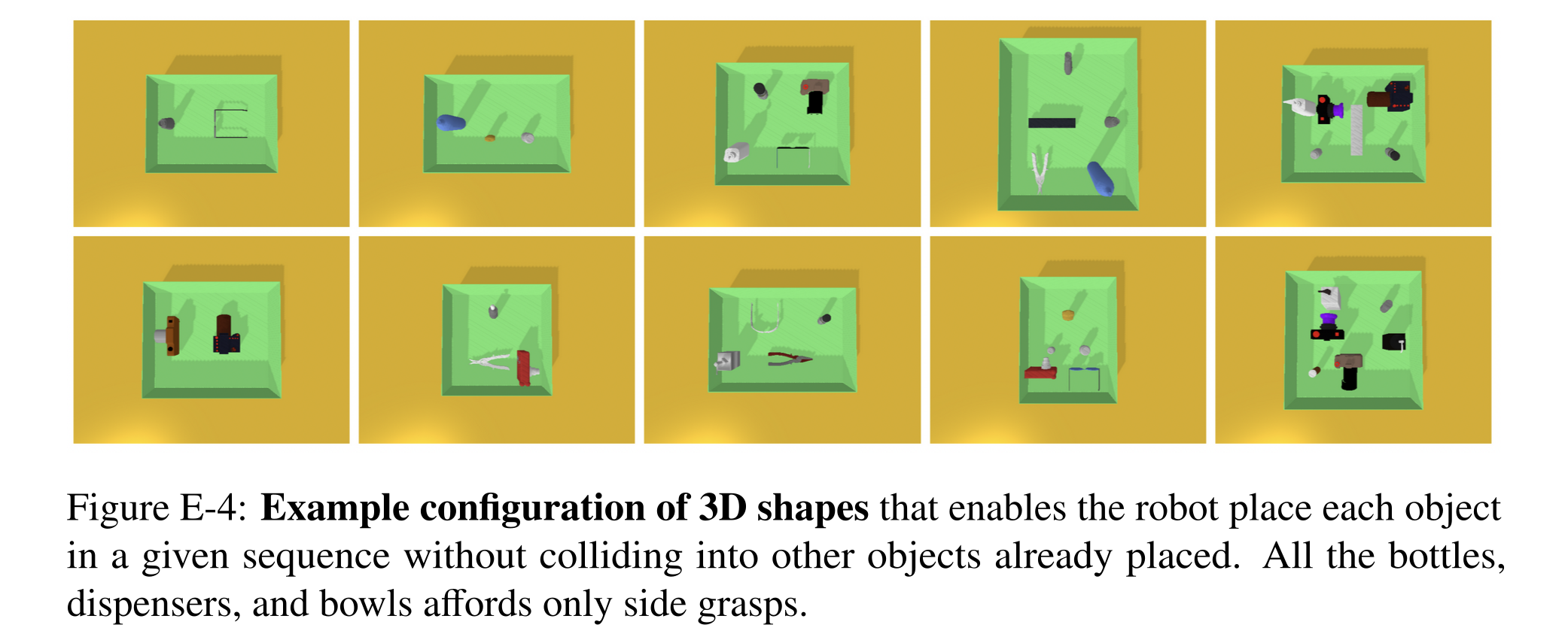
Figure E-4: Example configuration of 3D shapes that enables the robot place each object in a given sequence without colliding into other objects already placed. All the bottles, dispensers, and bowls affords only side grasps.
Discussion: Sample Complexity of Diffusion-CCSP
Each domain requires roughly 10,000–30,000 solution examples. Simulation supplies geometric/physical data cheaply in this study; learning human qualitative preferences would require annotation or other data sources. The appendix proposes sim-to-real transfer, but these experiments do not test the claim that transfer is effortless under real perception, contact, and model errors.
Discussion: Partial Observability
All reported experiments assume known object shapes and initial poses. Completing partial point clouds and replanning after detected collisions is proposed as a possible extension. No belief-space method, uncertainty model, or partial-observation evaluation is supplied.
Implementation and Training Details
Models use 1,000 diffusion steps, except robot-packing Diffusion-CCSP uses 500; encoders use 256-dimensional features normalized to the container. The implementation averages incident factor outputs in embedding space before pose decoding, while the main formulation writes a sum of denoising scores. Langevin sampling uses ten inner steps and a cosine-schedule-dependent step size. StructDiffusion uses a four-layer, two-head transformer without language embeddings; sequential rejection allows 50 pose proposals per object. These implementation choices should be preserved alongside the ideal energy-product explanation.
Discussion: Individual Constraint Diffusion Training and Finetuning
Constraint modules can in principle be trained separately or jointly, then recombined. The reported experiments train them concurrently because each scene supplies multiple interacting constraints. Finetuning for new data or shapes is suggested, without a reported adaptation study here.
Discussion: Weights for Energy Function Composition
All constraint weights are set to one. The authors attribute successful composition to steep learned feasible-region energies and joint training over combined constraints. This is an empirical choice on the tested domains, not a general solution to balancing incompatible scales or competing constraints.
Discussion: Local Optima in Optimization
Multiple random initial noises are sampled in parallel to reduce sensitivity to poor local optima. Physical simulators check collision and stability in the relevant domains; learned classifiers are proposed where exact checkers are unavailable. Repeated seeds improve practical success but neither prove infeasibility after failure nor guarantee a valid sample.
Failure Case Analysis
Failures include object intersections, missed qualitative relations, unstable stacks, and incorrect support structure. Across 4,000 samples on 400 qualitative problems, narrower/disconnected valid regions and less abundant training examples correlate with more violations. A two-object area estimate helps illustrate this trend but does not capture crowded-scene collision geometry, so collision-free constraints are excluded from that interpretation.
Additional Sampler Comparison
The extended evaluation permits 100 samples per problem and marks instances still unsolved, revealing that additional attempts do not eliminate every failure. Direct reverse diffusion is faster; Langevin sampling generally improves difficult compositional cases at extra cost. Table E.1 reports average per-instance time within a batch of 100 (roughly 0.01–0.04 seconds reverse versus 0.06–0.19 seconds Langevin), which should not be read as single-request wall-clock latency.
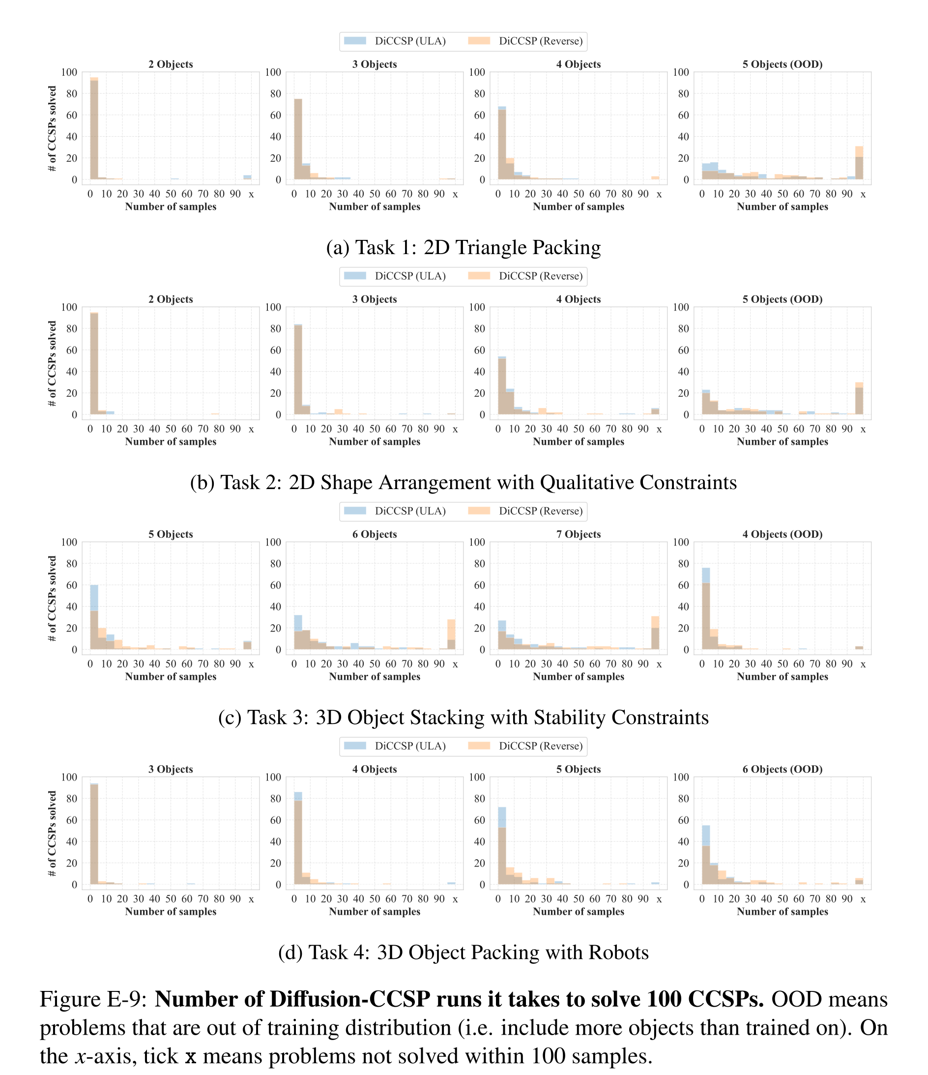
Figure E-9: Number of Diffusion-CCSP runs it takes to solve 100 CCSPs. OOD means problems that are out of training distribution (i.e. include more objects than trained on). On the x-axis, tick x means problems not solved within 100 samples.
Integration with Task and Motion Planning Algorithms
A high-level search chooses a discrete plan skeleton; action preconditions and the goal induce constraints on continuous grasps, placements, and trajectories. A satisfying assignment instantiates the skeleton, while unsuccessful continuous solving prompts another candidate. The pick-place example shows how later collision checks depend on earlier selected poses. Diffusion-CCSP is the continuous proposal component within this broader planner, with external validity checking and motion planning retained.
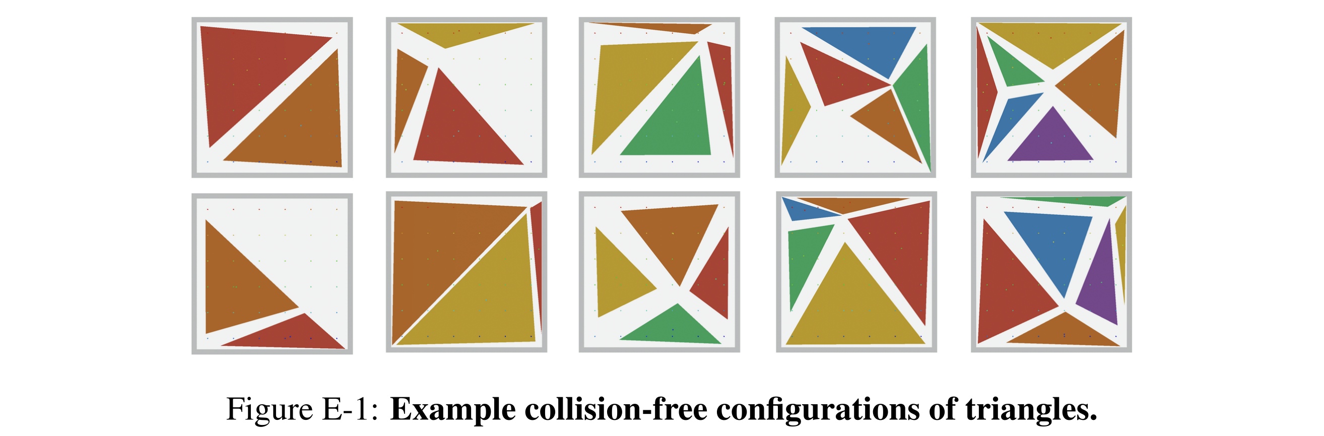
Figure E-1: Example collision-free configurations of triangles.
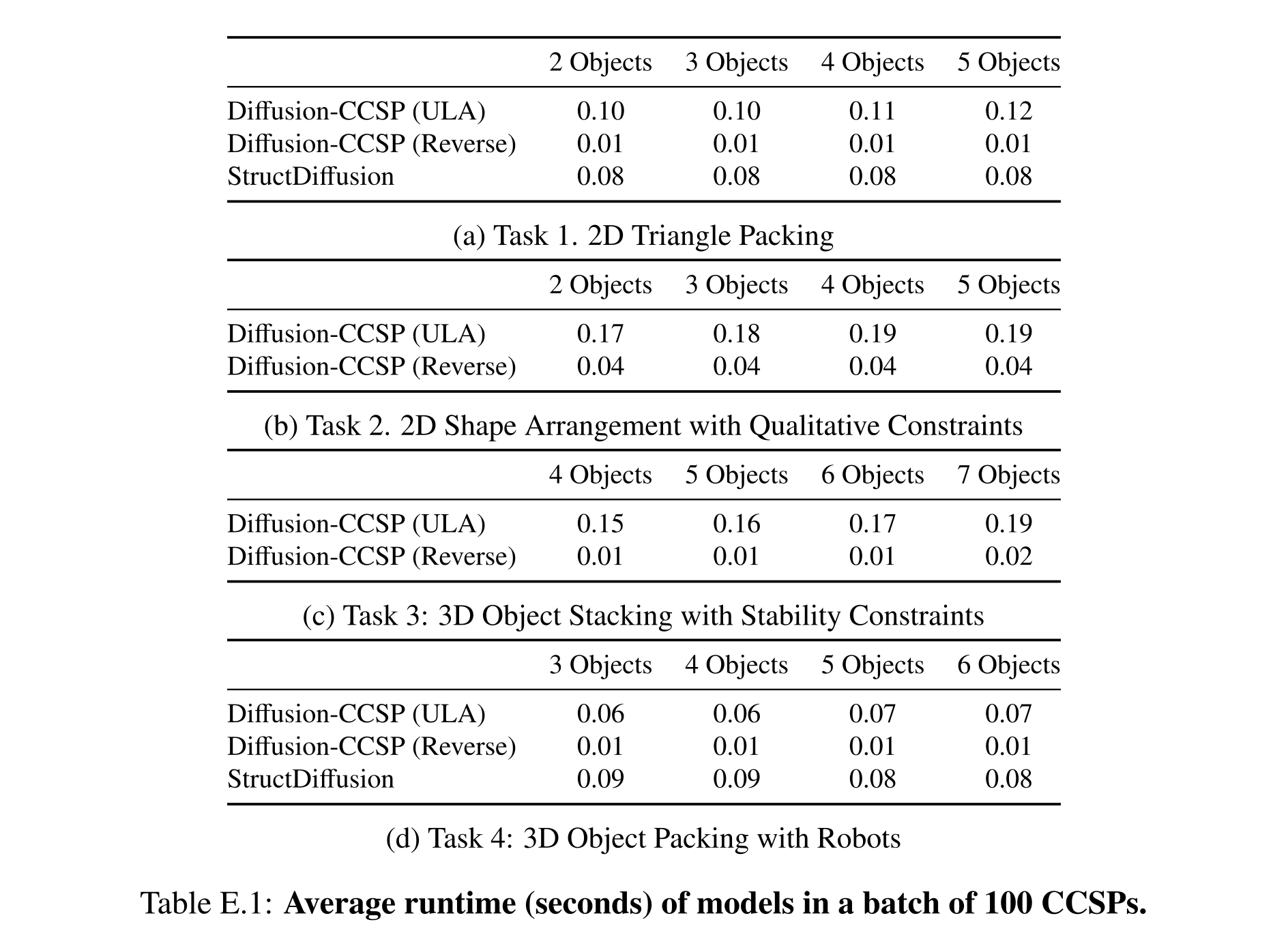
Table E.1: Average runtime (seconds) of models in a batch of 100 CCSPs.
Learned Gradient Fields
The visualizations cover all thirteen geometric/qualitative constraint types: six object-container and seven object-object relations. Energy and gradient slices use fixed square sizes and a fixed reference object; sampled poses and training distributions are shown alongside them. Steep low-energy regions qualitatively match feasible regions, but the plots are specific slices and do not certify the joint solver. The appendix’s late-placed figures also retain the full failure examples, runtime table, and task-and-motion action/graph diagrams.
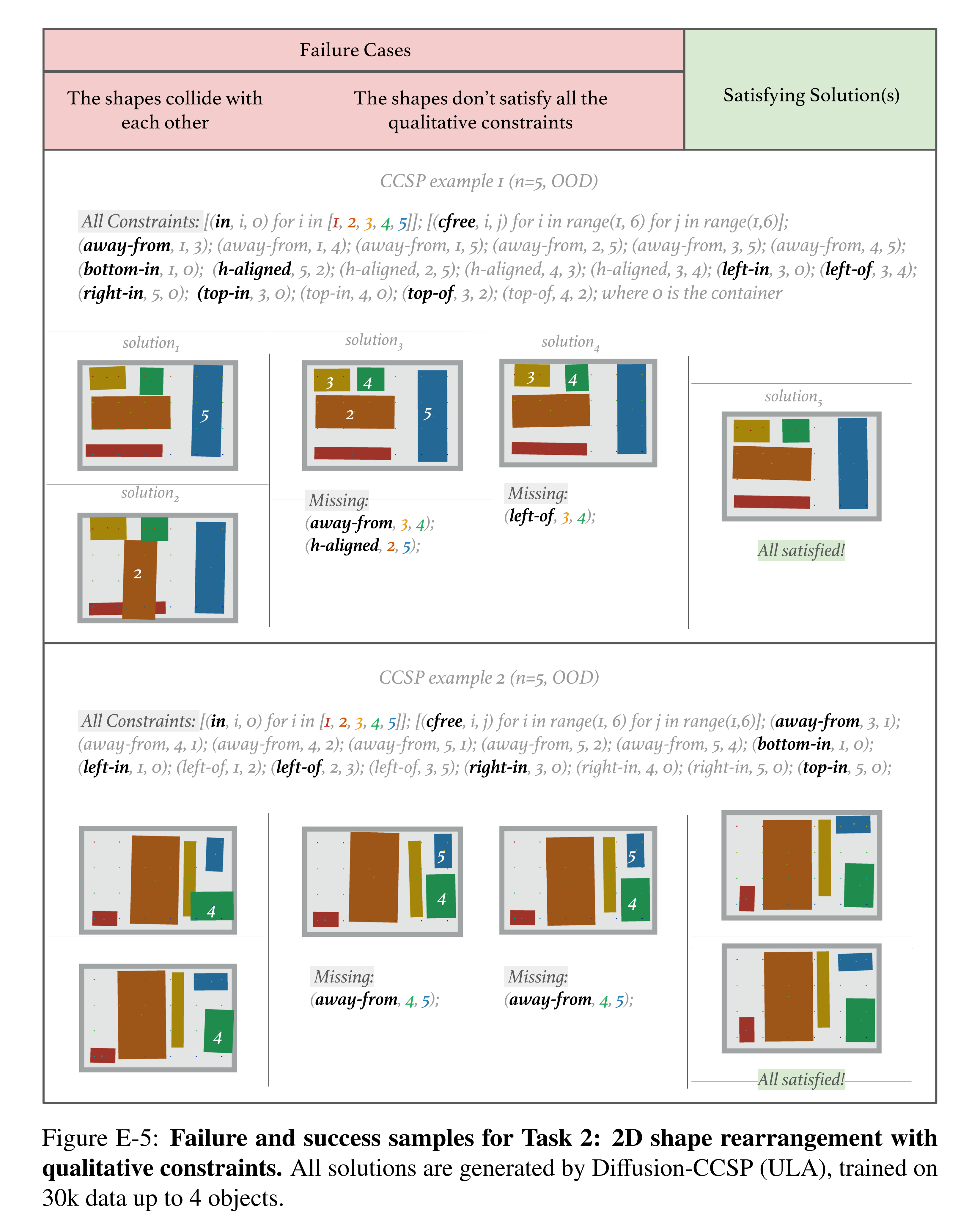
Figure E-5: Failure and success samples for Task 2: 2D shape rearrangement with qualitative constraints. All solutions are generated by Diffusion-CCSP (ULA), trained on 30k data up to 4 objects.
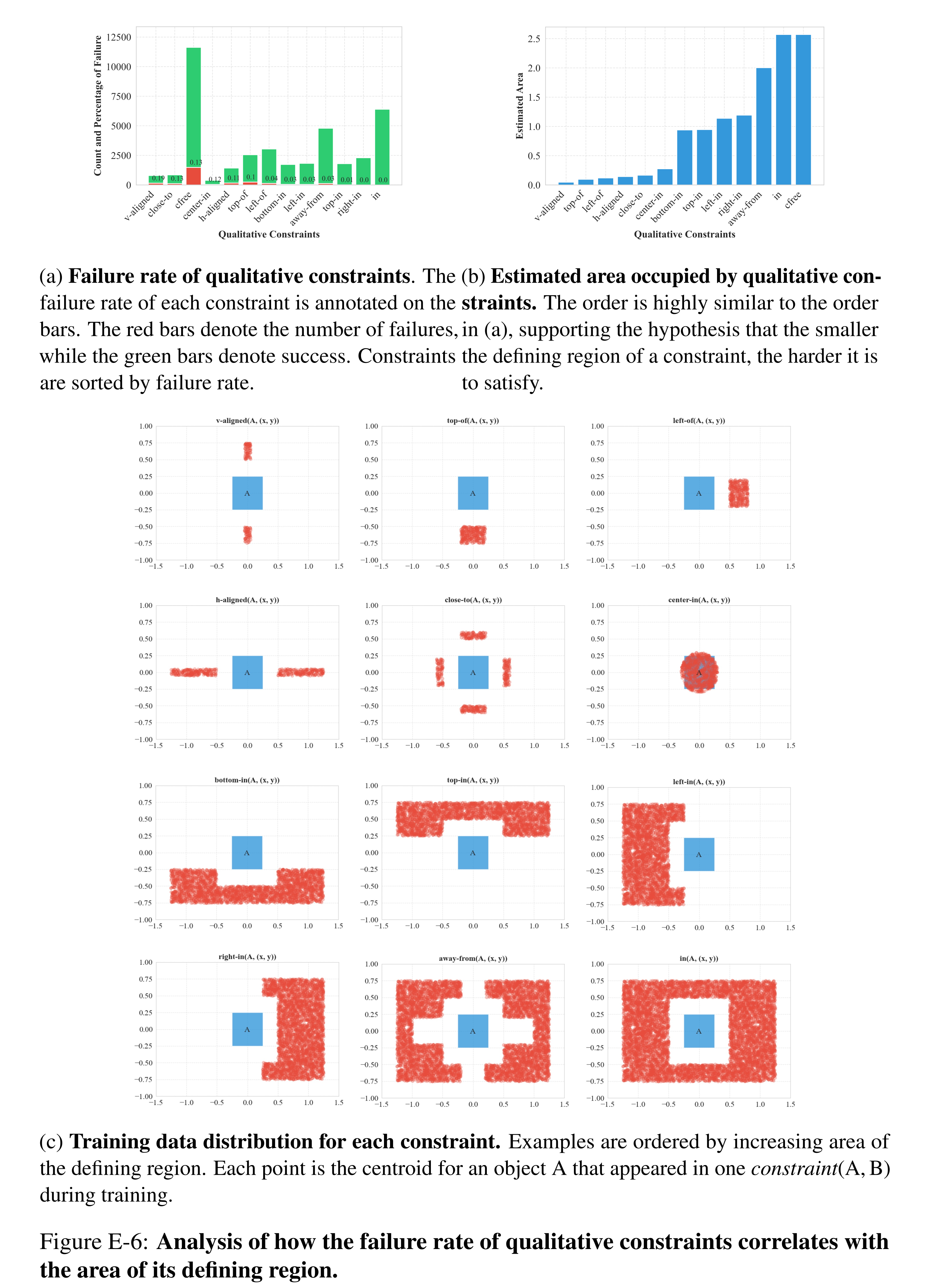
Figure E-6: Analysis of how the failure rate of qualitative constraints correlates with the area of its defining region.
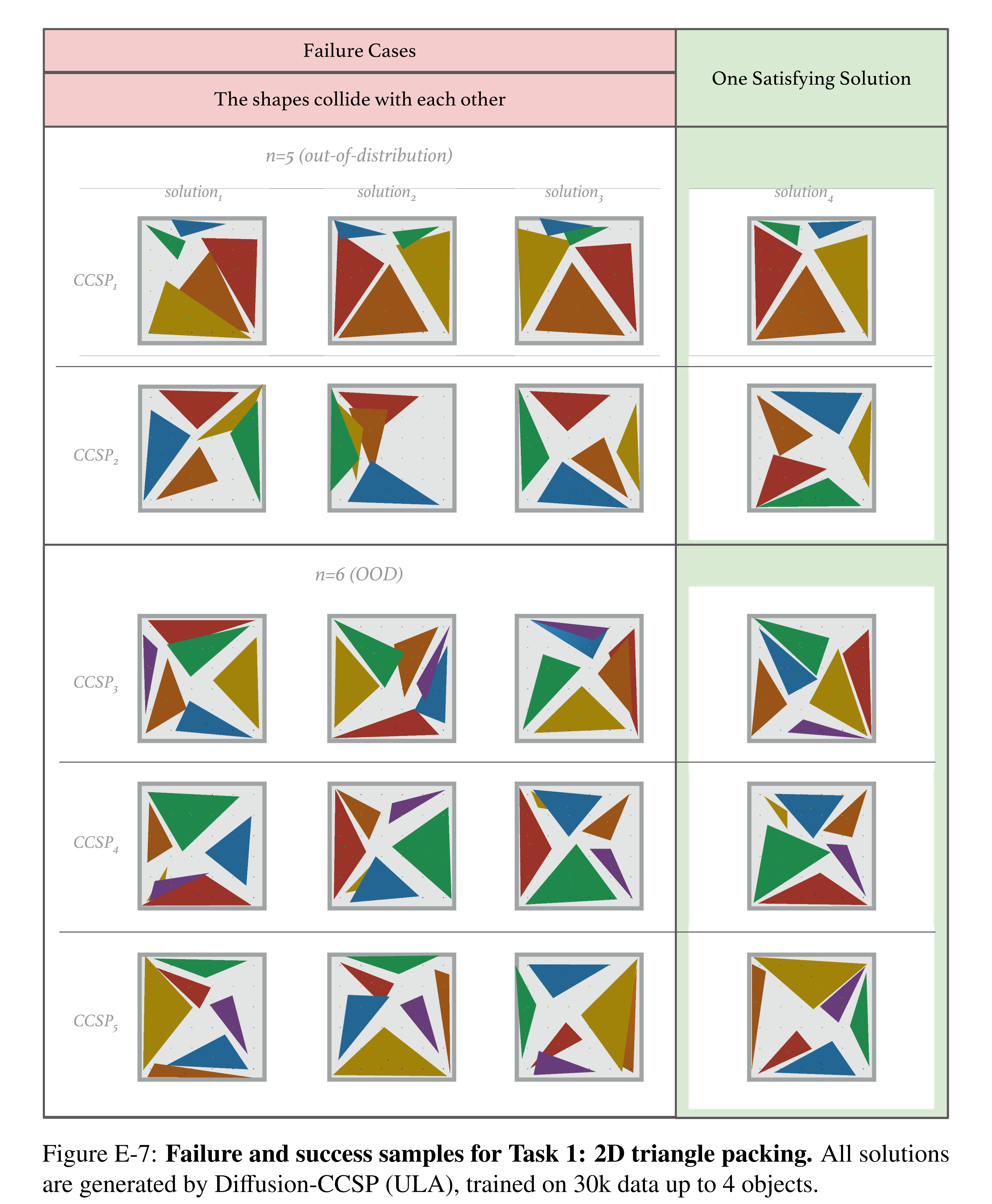
Figure E-7: Failure and success samples for Task 1: 2D triangle packing. All solutions are generated by Diffusion-CCSP (ULA), trained on 30k data up to 4 objects.
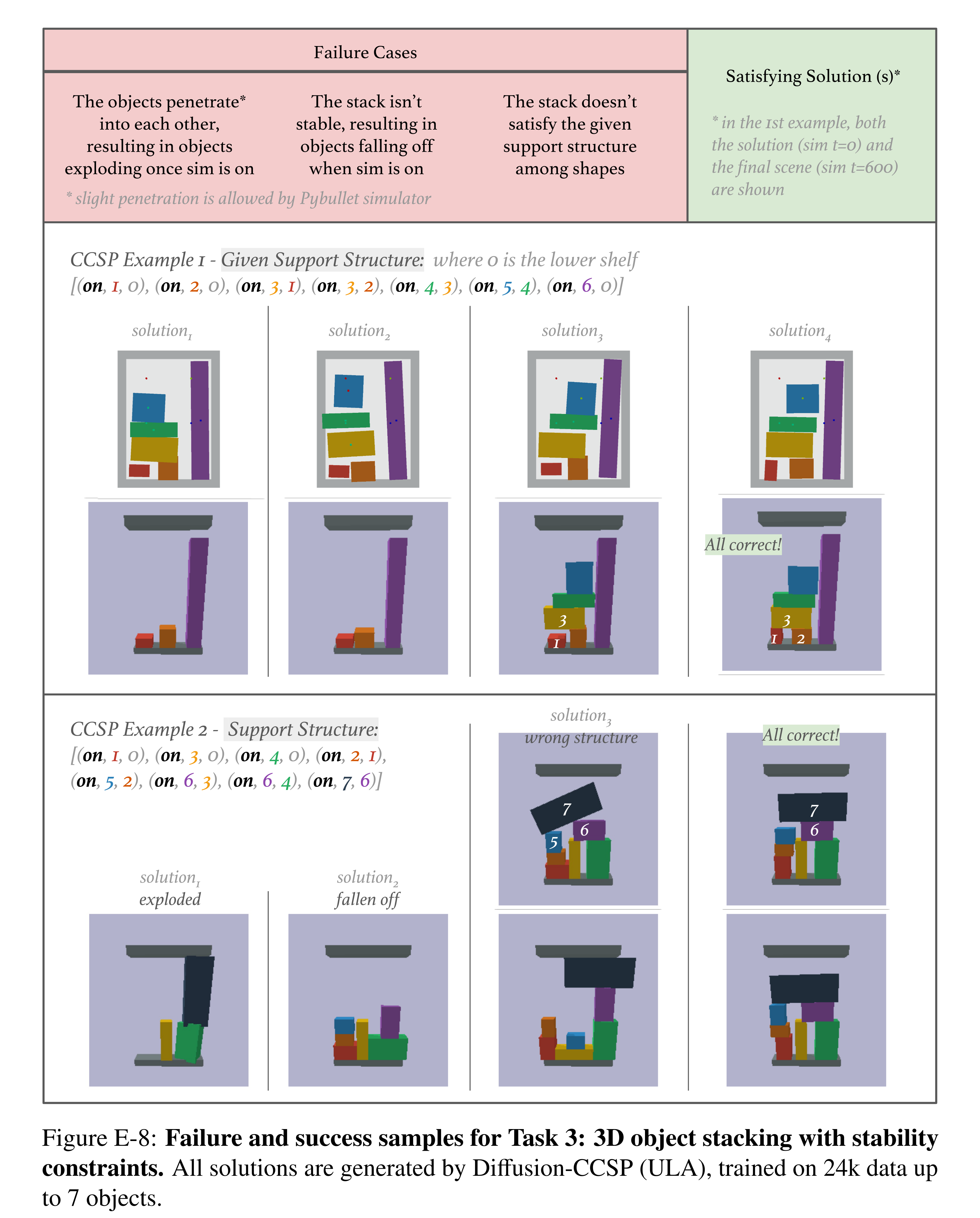
Figure E-8: Failure and success samples for Task 3: 3D object stacking with stability constraints. All solutions are generated by Diffusion-CCSP (ULA), trained on 24k data up to 7 objects.
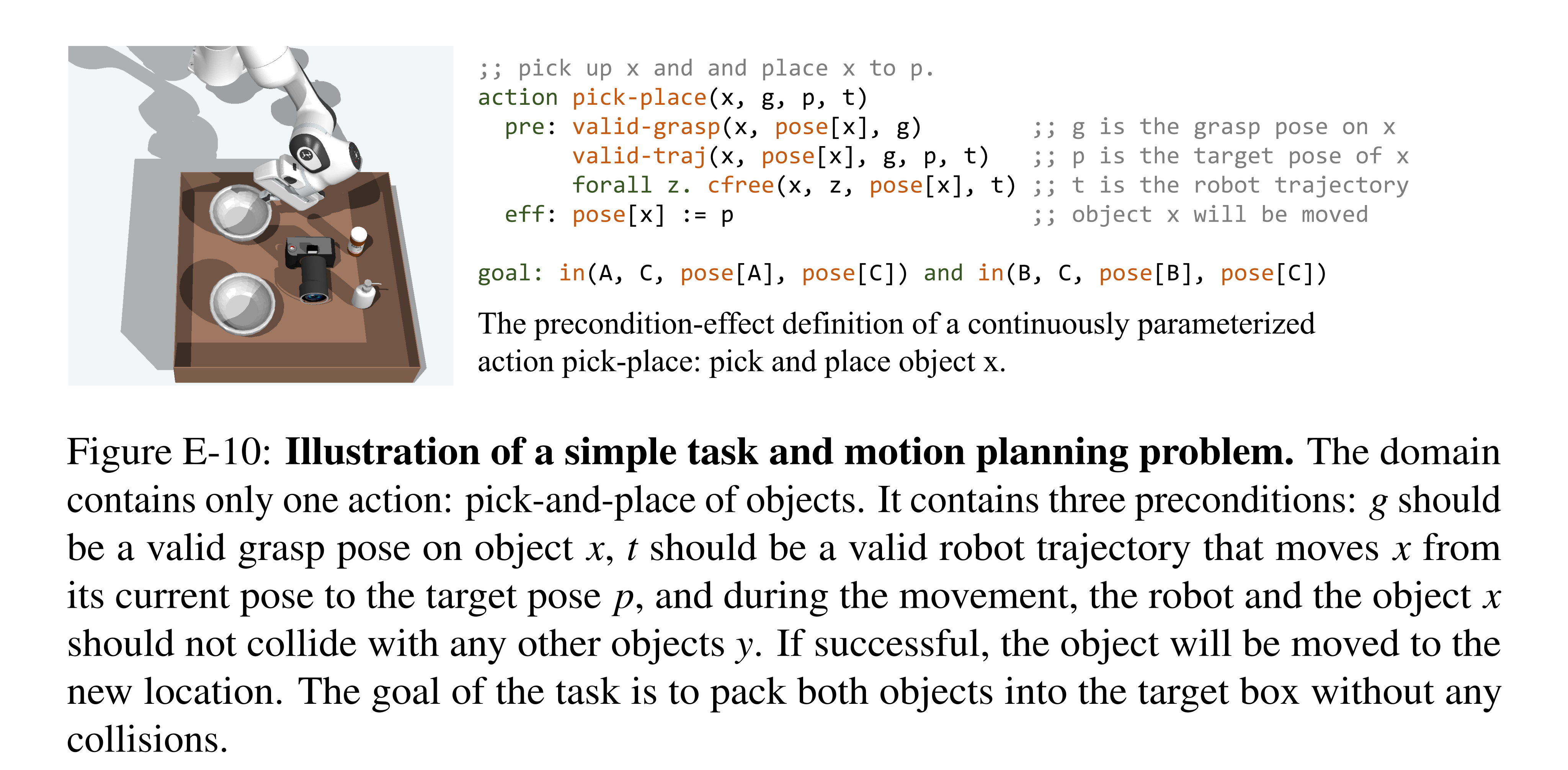
Figure E-10: Illustration of a simple task and motion planning problem. The domain contains only one action: pick-and-place of objects. It contains three preconditions: g should be a valid grasp pose on object x, t should be a valid robot trajectory that moves x from its current pose to the target pose p, and during the movement, the robot and the object x should not collide with any other objects y. If successful, the object will be moved to the new location. The goal of the task is to pack both objects into the target box without any collisions.
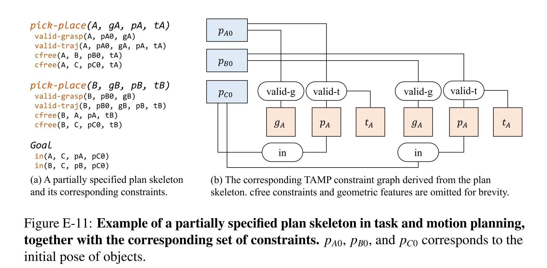
Figure E-11: Example of a partially specified plan skeleton in task and motion planning, together with the corresponding set of constraints. pA0, pB0, and pC0 corresponds to the initial pose of objects.
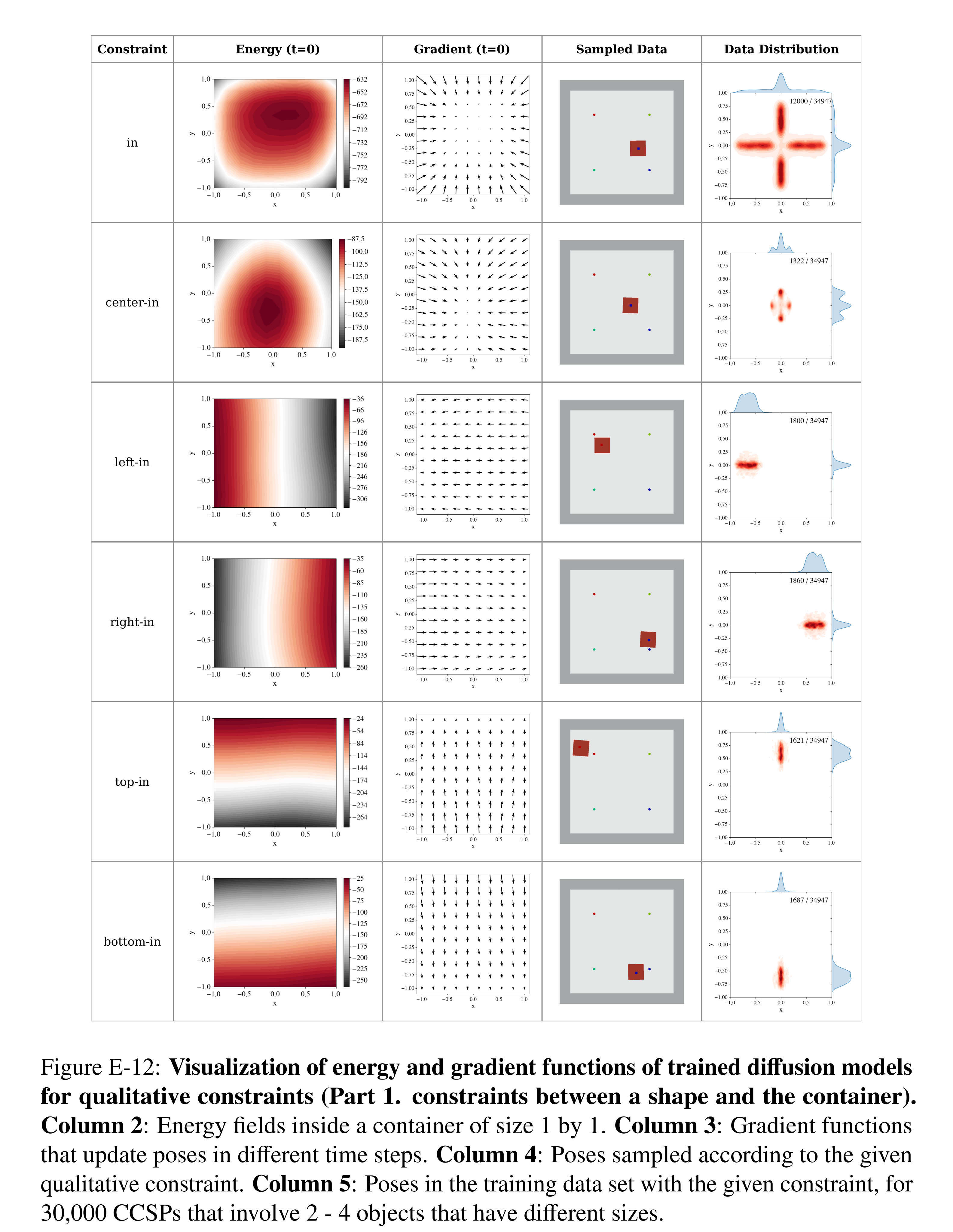
Figure E-12: Visualization of energy and gradient functions of trained diffusion models for qualitative constraints (Part 1. constraints between a shape and the container). Column 2: Energy fields inside a container of size 1 by 1. Column 3: Gradient functions that update poses in different time steps. Column 4: Poses sampled according to the given qualitative constraint. Column 5: Poses in the training data set with the given constraint, for 30,000 CCSPs that involve 2 - 4 objects that have different sizes.
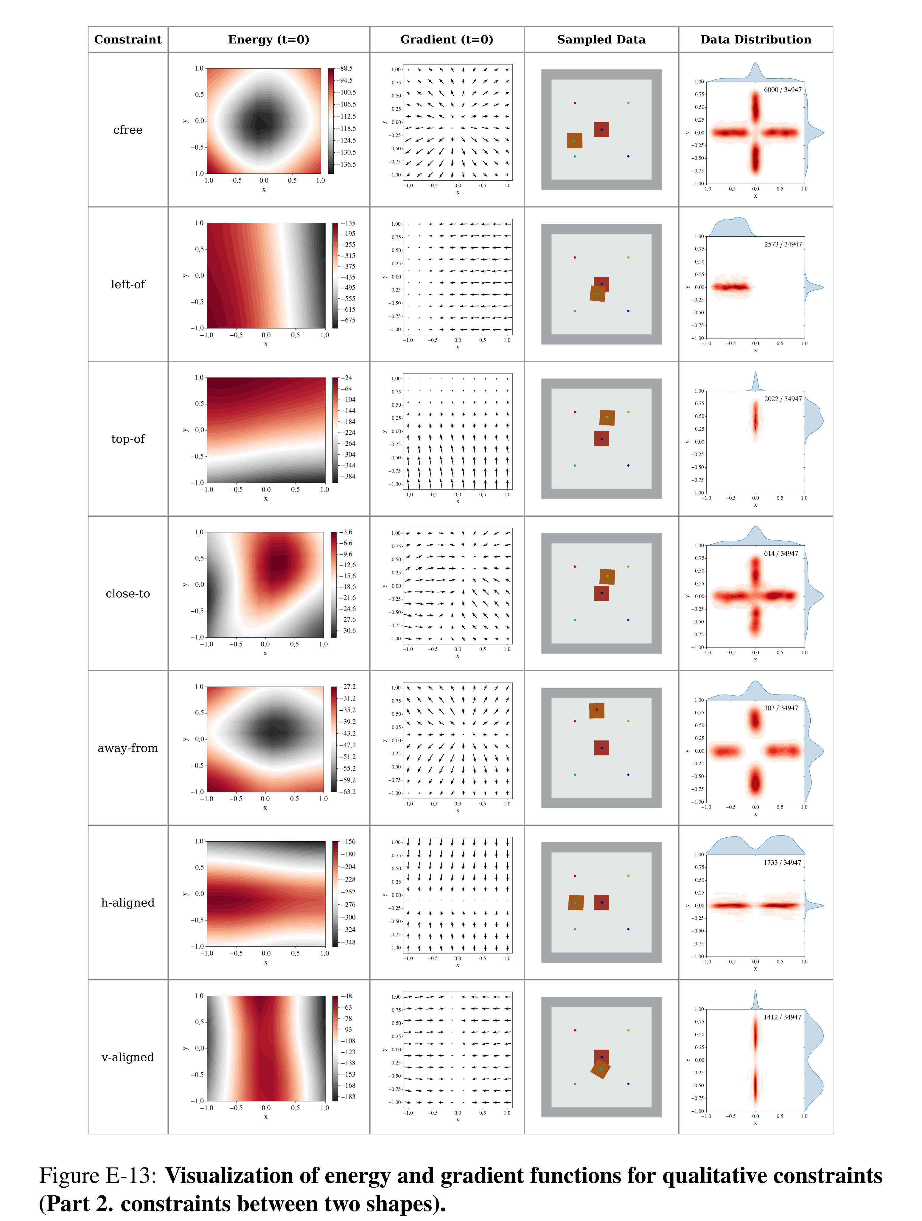
Figure E-13: Visualization of energy and gradient functions for qualitative constraints (Part 2. constraints between two shapes).
Appendix for Visual Concept Learning
Appendix F specifies the CLEVR language and executor, parser architecture and optimization, curriculum, ablations, domain extensions, and success/failure traces.
CLEVR Domain-Specific Language
The typed DSL distinguishes objects, object sets, concepts, attributes, relations, integers, and Booleans. Object-taking operations require a unique referent; an implicit Unique conversion handles an appropriate set. Tables F.1–F.2 retain the full signatures. The Exist description says “empty,” but its implementation and usage test whether an object exists.
Semantic Parsing
The recursive parser decodes an operation, optionally selects its concept argument, then creates child states for up to two non-concept arguments. Word embeddings combine 256 learned dimensions with 128 positional dimensions; a two-layer bidirectional GRU encodes the sentence. Feed-forward operation/concept decoders and GRU child encoders construct the program tree.
Concept words and their types are extracted with hand-coded rules in CLEVR. Type-based input embeddings permit a known grammar to accept a new concept word; consecutive object concepts are grouped into one filter. Parser word embeddings are distinct from visual concept embeddings. Algorithm 12 and the running example retain the recursive procedure and intermediate decoding states.
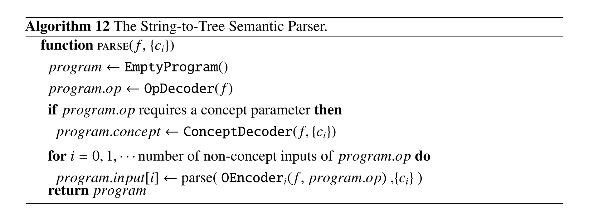
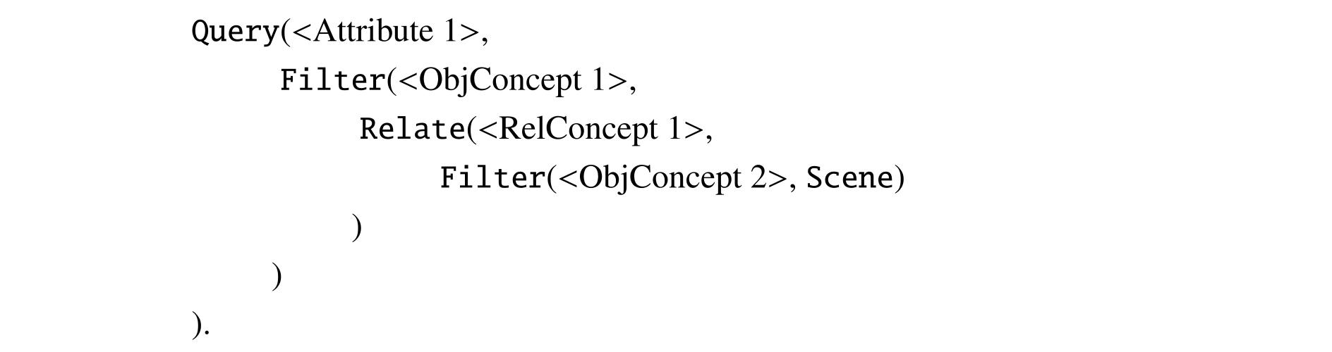
Program Execution
An Object is a normalized distribution over detections; an ObjectSet has independent soft memberships. Unique applies softmax to membership logits. Learned attribute-assignment weights and cosine-based classifiers produce object, relational, and same-attribute scores.
Filtering/intersection use minimum, union uses maximum, relations use weighted sums, existence uses maximum membership, and counting sums memberships. Query normalizes over applicable concepts; numeric comparisons use scaled sigmoids. Table F.4 retains every operator and constants 0.5/0.25. Probabilities are stored in log space for stability; these fuzzy operations are computational relaxations rather than a full joint probabilistic model.
Equations


Optimization of the Semantic Parser
With perception fixed, enumerate programs consistent with the question’s concept set and retain those producing the right answer. The parser then learns from this answer-consistent set rather than noisy on-policy samples. Equivalent programs and scene-specific accidental answers can both enter the set.
A stop-gradient parser-probability weight reduces the influence of low-probability candidates during likelihood optimization. Additional scenes can expose accidental programs, but answer consistency in a finite dataset does not guarantee that every remaining program matches the intended semantics.
Equation



Equations


Curriculum Learning Setup
Three lessons add depth-3 object questions, shallow relational questions, then full CLEVR programs, while scene size grows from three to ten objects. Object grounding is frozen in the relational lesson; perception is initially frozen during complex parsing. Relation-count questions are added because original CLEVR templates insufficiently isolate relational concepts.
The source reports failure to learn without either object-count or question-complexity curriculum. Curriculum selection itself uses latent program depth, even though target programs are not used as parser supervision. Lesson 1 is described as three question types but enumerates four.
Ablation Study
The ablations examine execution-based parsing accuracy, ImageNet initialization, training-data quantity, and object/mask representations for baseline architectures.
Semantic parsing accuracy.
Programs are executed on ground-truth object annotations; incorrect, invalid, or ambiguous executions count as failures. Accuracy exceeds 99.9%. Because behaviorally equivalent programs are accepted, this number is execution-answer accuracy rather than exact program-match accuracy.
Impacts of the ImageNet pre-training.
Random feature initialization lowers shape classification from 98.7% to 97.5% and QA from 98.9% to 98.2%. The latter is a 0.7-point drop, differing from the main text’s 0.5-point description. This ablation does not remove the separately pretrained object detector.
Data Efficiency and Object-based Representations
Object-feature baselines pad to twelve detections and concatenate region/context features. Replacing TbD’s spatial convolutions with 1D operations over an object list loses appropriate permutation structure; attention pooling in MAC does not directly count arbitrary sets. Their poor results therefore do not show that object representations alone are harmful.
Mask-guided attention converges faster without improving final accuracy. NS-CL benefits from programmed execution rather than learning all operations from examples. Full-data experiments reserve 3,500 training images for model selection and report 99.2% on CLEVR validation.
Extending to Other Scene and Language Domains
The domain extensions separately adapt the DSL and perception/parsing pipeline to Minecraft scenes and grounded natural-image questions.
Minecraft Dataset
The Minecraft dataset contains 10,000 scenes with three to six objects, twelve categories, and four facing directions. FilterMost selects an extremal object such as the closest, and BelongTo tests membership. NS-CL reaches 93.3% overall versus NS-VQA’s 87.7%, a 5.6-point difference. Detection/occlusion errors remain; the source attributes some baseline degradation to noisy box-to-annotation matching.
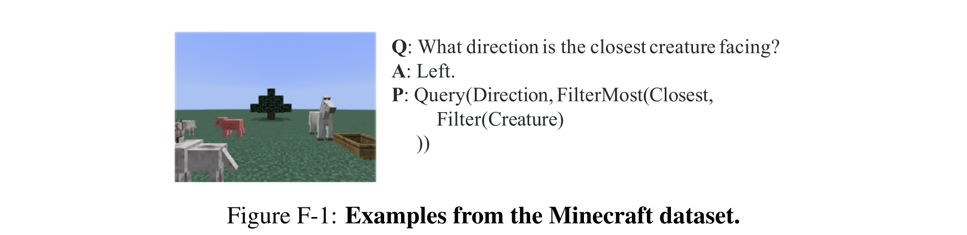
Figure F-1: Examples from the Minecraft dataset.
VQS Dataset
VQS training uses 63,509 images, with another 5,000 for validation, and ranks eighteen candidate answers per question. A pretrained dependency parser extracts programs; concept embeddings start from GloVe bag-of-words features. ResNet-34 image features support NS-CL, MLP, and adapted MAC comparisons. Results are comparable rather than superior to all baselines, while execution traces expose several error sources.
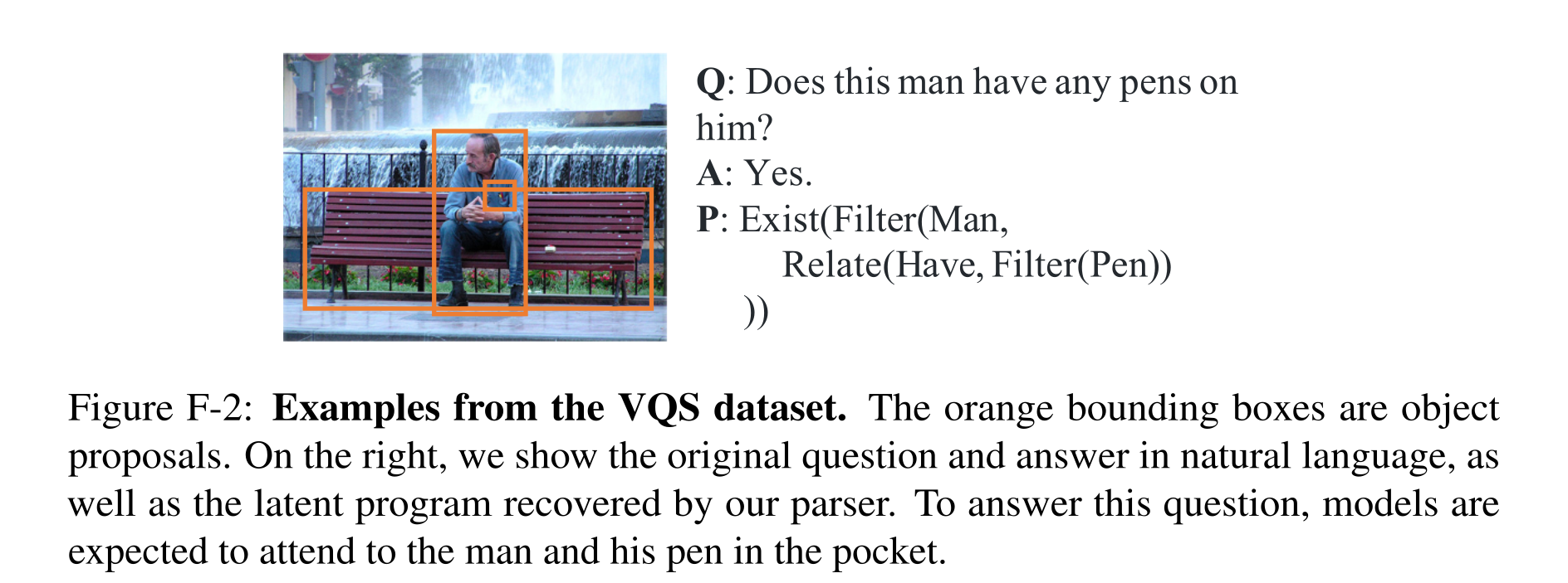
Figure F-2: Examples from the VQS dataset. The orange bounding boxes are object proposals. On the right, we show the original question and answer in natural language, as well as the latent program recovered by our parser. To answer this question, models are expected to attend to the man and his pen in the pocket.
Visualization of execution traces and visual concepts
The examples show correct CLEVR/Minecraft/VQS traces, missed detections, material misclassification, ambiguous referents, and incorrect activity recognition. A VQS example answers correctly while selecting the wrong object, directly showing that answer accuracy does not guarantee faithful grounding. Thresholded concept galleries illustrate learned categories, attributes, and relations; they are qualitative selections rather than unbiased accuracy estimates.
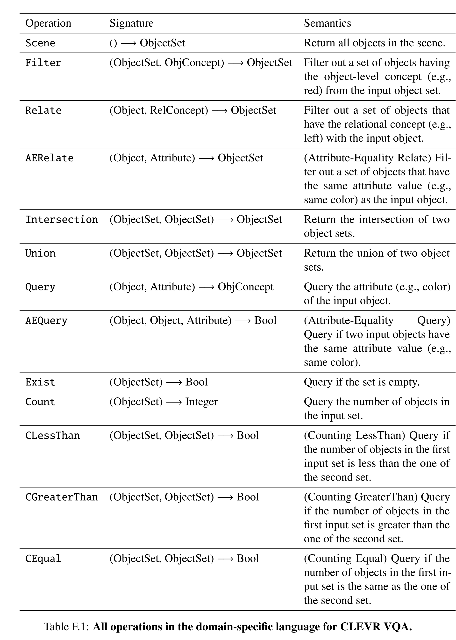
Table F.1: All operations in the domain-specific language for CLEVR VQA.
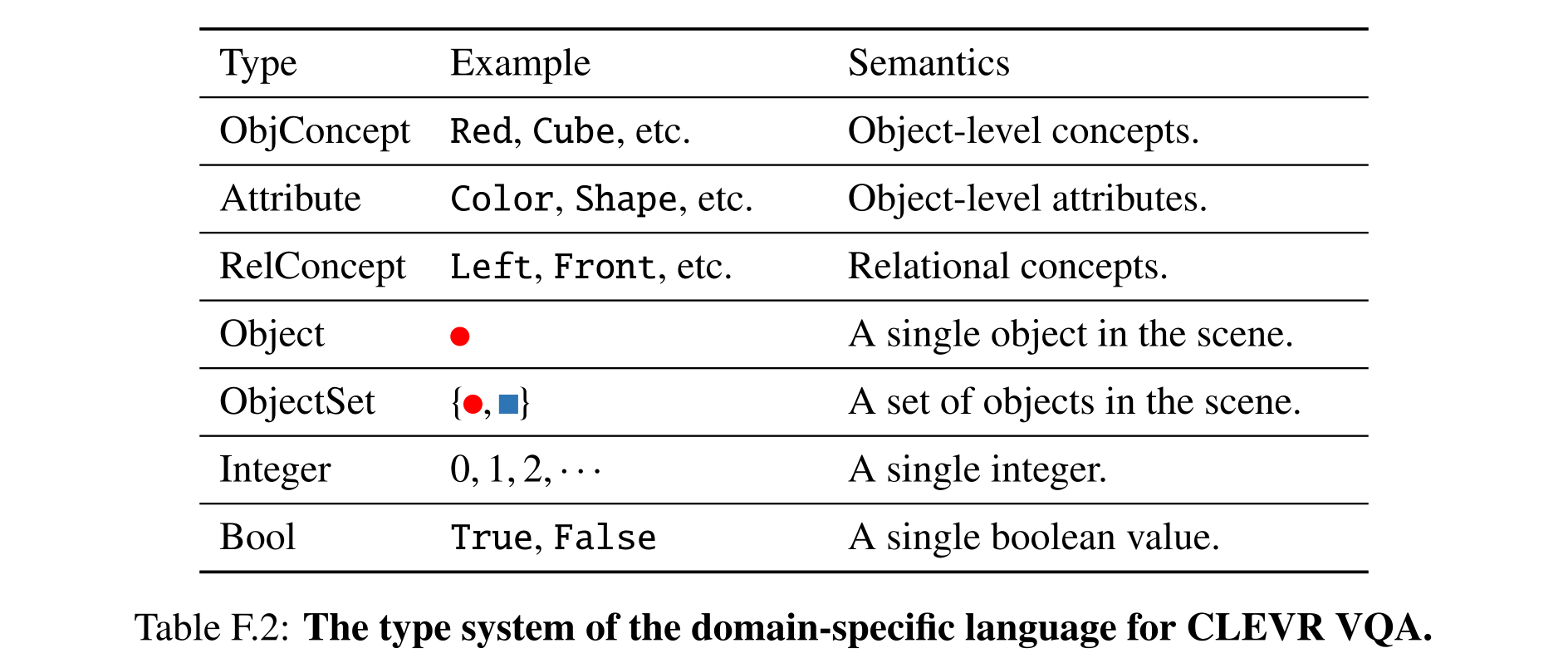
Table F.2: The type system of the domain-specific language for CLEVR VQA.
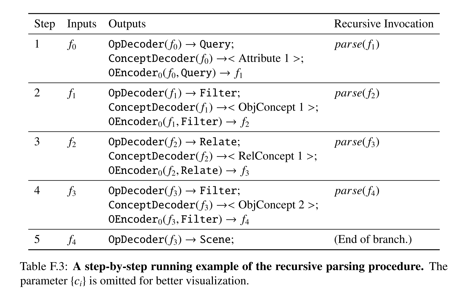
Table F.3: A step-by-step running example of the recursive parsing procedure. The parameter {ci} is omitted for better visualization.
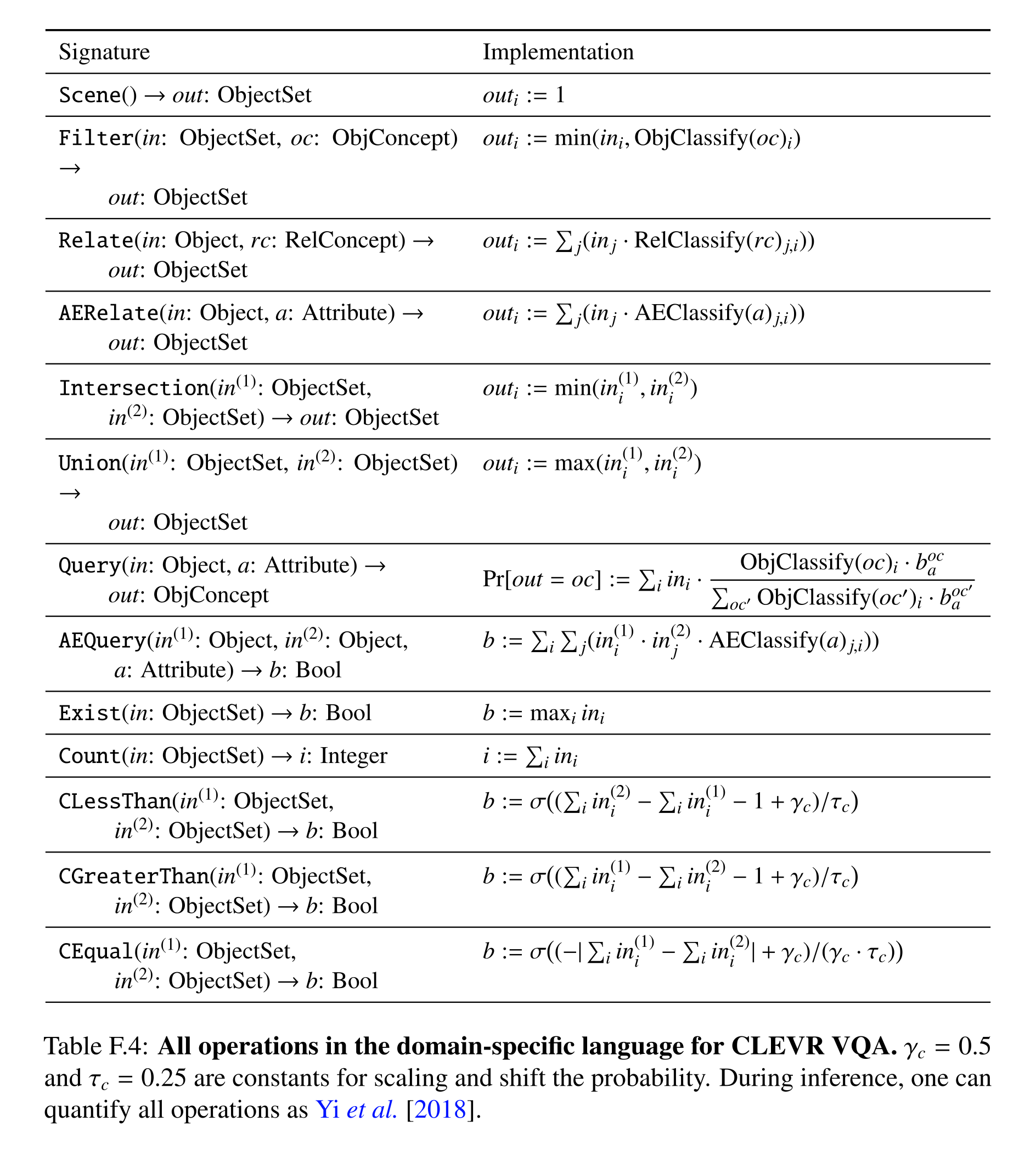
Table F.4: All operations in the domain-specific language for CLEVR VQA. γc = 0.5 and τc = 0.25 are constants for scaling and shift the probability. During inference, one can quantify all operations as Yi et al. [2018].
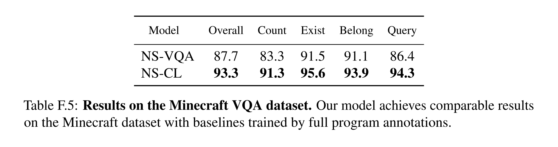
Table F.5: Results on the Minecraft VQA dataset. Our model achieves comparable results on the Minecraft dataset with baselines trained by full program annotations.
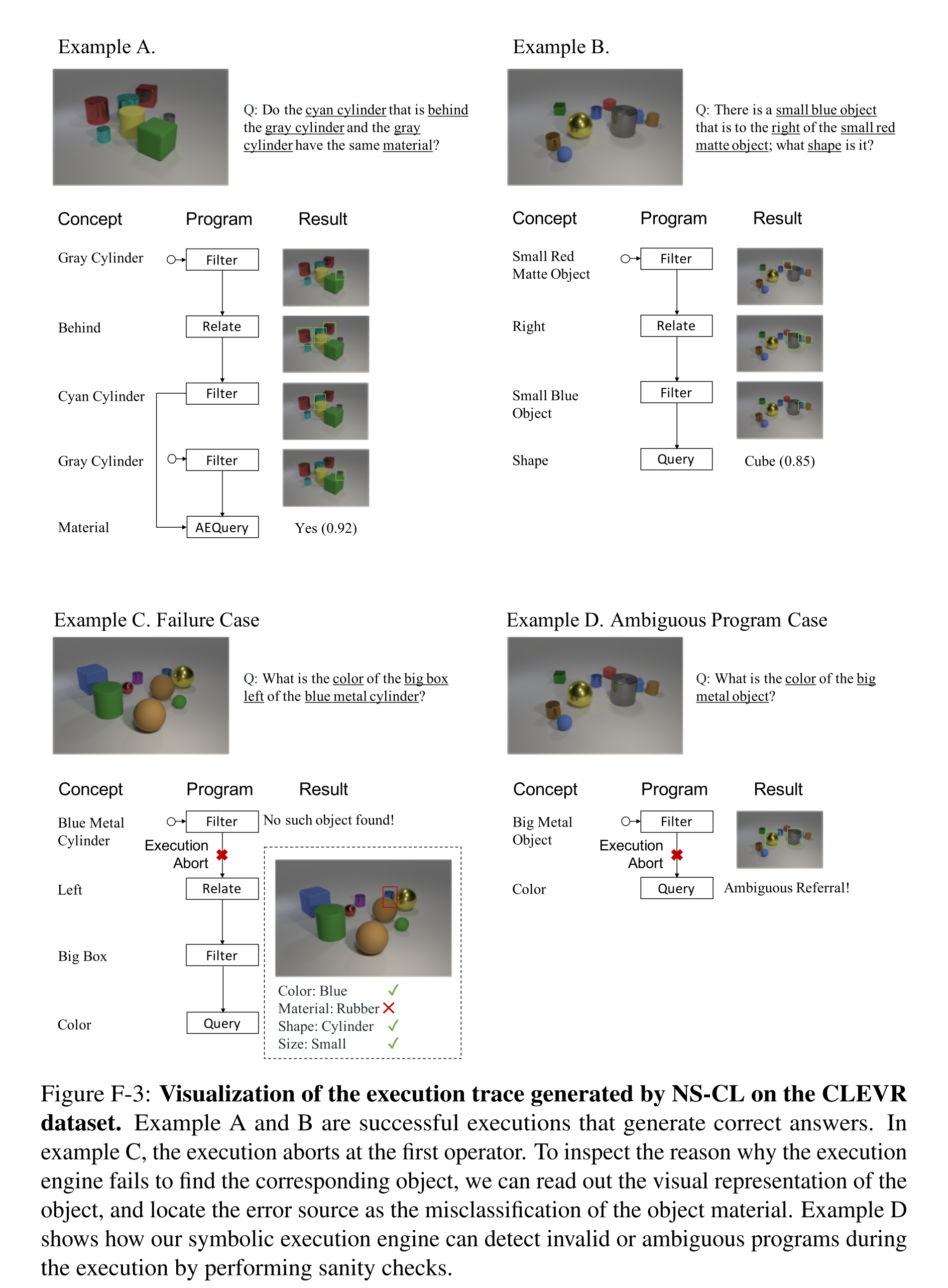
Figure F-3: Visualization of the execution trace generated by NS-CL on the CLEVR dataset. Example A and B are successful executions that generate correct answers. In example C, the execution aborts at the first operator. To inspect the reason why the execution engine fails to find the corresponding object, we can read out the visual representation of the object, and locate the error source as the misclassification of the object material. Example D shows how our symbolic execution engine can detect invalid or ambiguous programs during the execution by performing sanity checks.
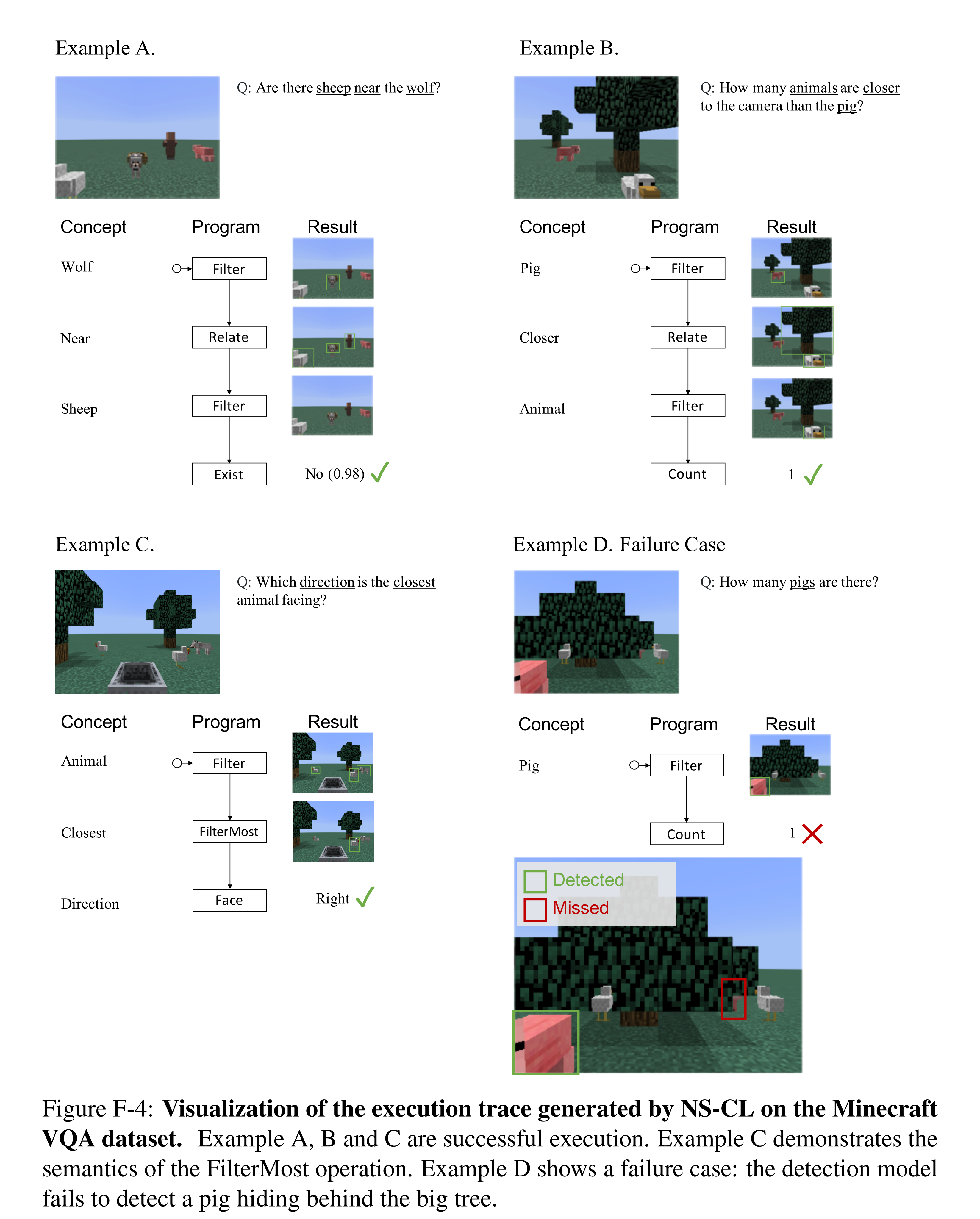
Figure F-4: Visualization of the execution trace generated by NS-CL on the Minecraft VQA dataset. Example A, B and C are successful execution. Example C demonstrates the semantics of the FilterMost operation. Example D shows a failure case: the detection model fails to detect a pig hiding behind the big tree.
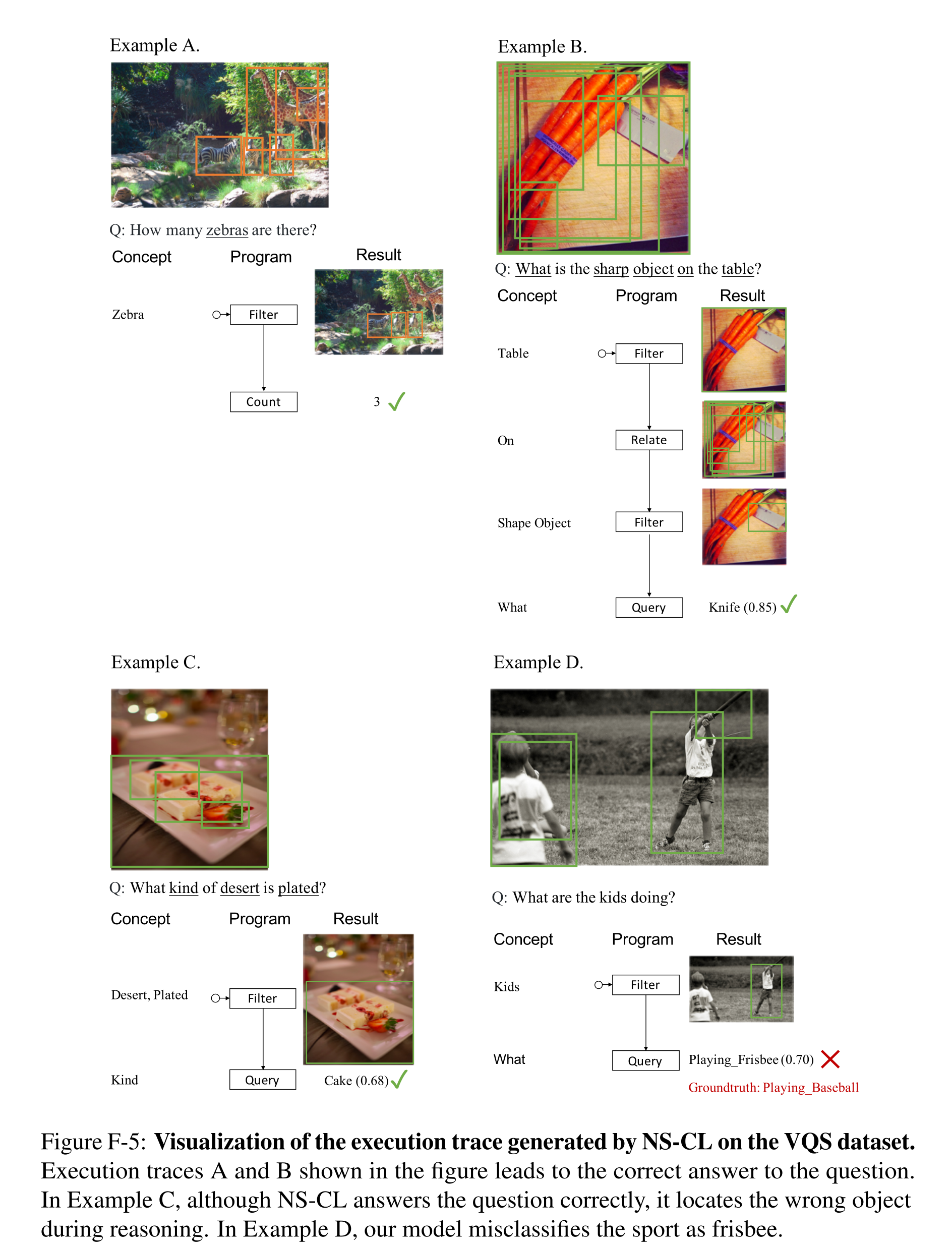
Figure F-5: Visualization of the execution trace generated by NS-CL on the VQS dataset. Execution traces A and B shown in the figure leads to the correct answer to the question. In Example C, although NS-CL answers the question correctly, it locates the wrong object during reasoning. In Example D, our model misclassifies the sport as frisbee.
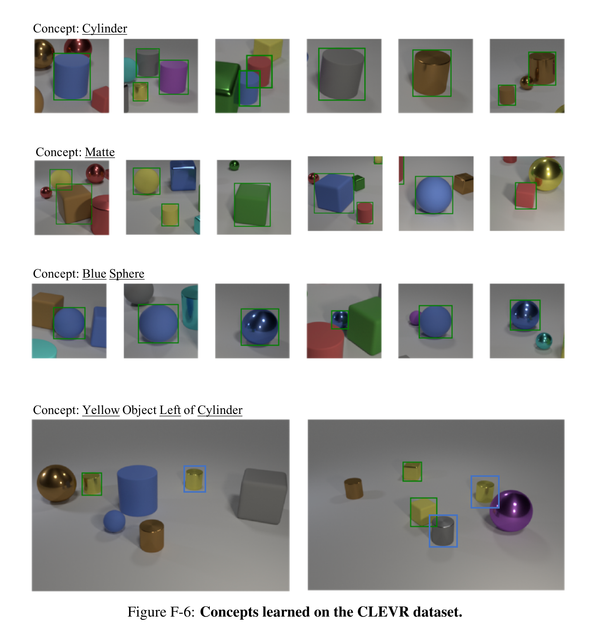
Figure F-6: Concepts learned on the CLEVR dataset.
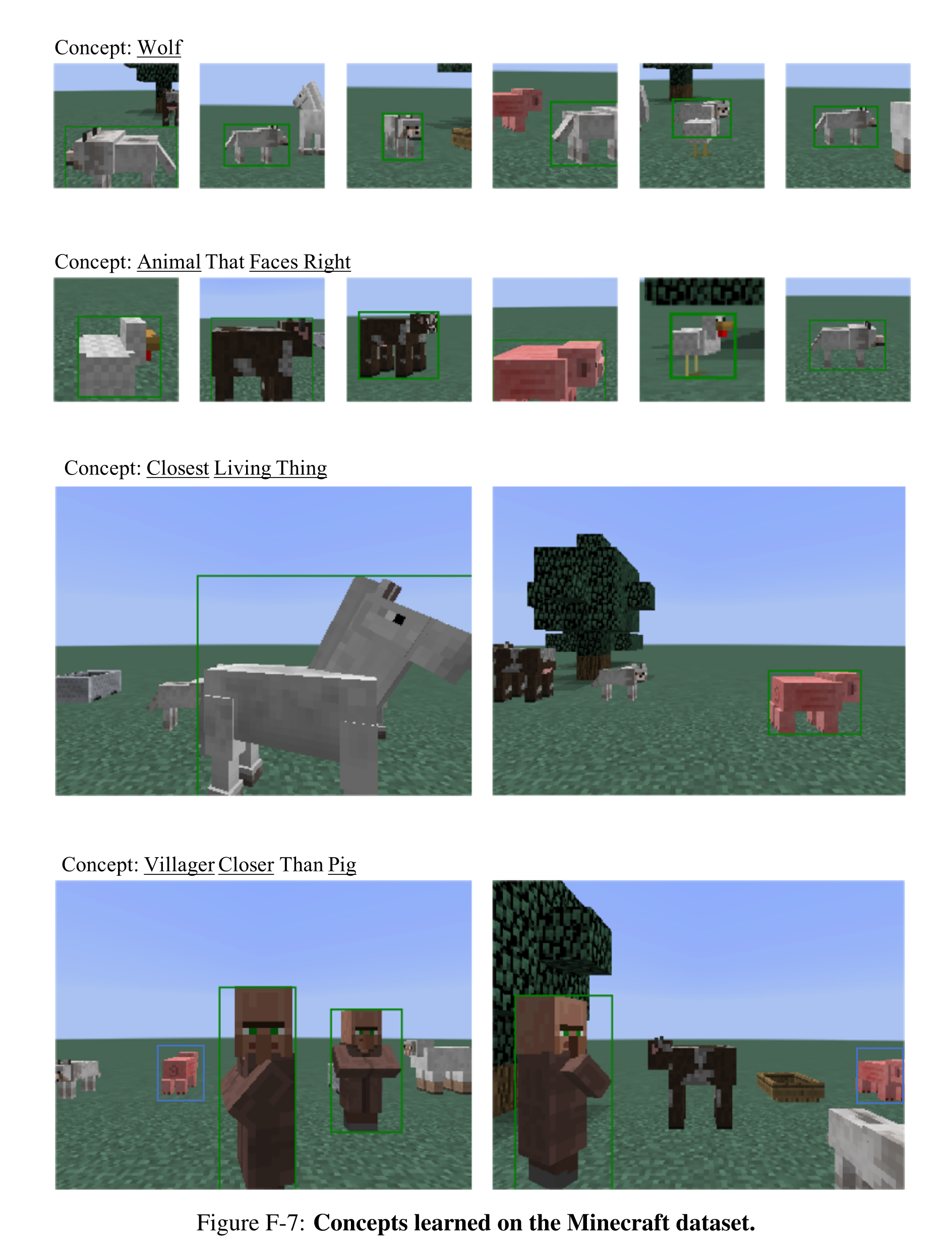
Figure F-7: Concepts learned on the Minecraft dataset.
Appendix for Fast Visual Concept Learning with Metaconcepts
The appendix specifies FALCON’s embedding distributions, graph and recurrent updates, supervised parsers, training schedules, dataset construction, ablations, and failure cases. These details qualify the fast-learning claim: new concepts are inferred quickly using modules and base concepts learned beforehand.
Model Details
Implementation details separate persistent concept inference from downstream question answering. The same executor can reuse an inferred concept across multiple images and questions; the sections below define the representation, inference network, parsing supervision, and baseline implementations.
Remarks on the overall model structure
A concept embedding compresses its visual examples and supplemental relationships into a library entry. At inference time, questions use that entry rather than processing all original examples again. This is the architectural distinction between concept-centric models and end-to-end baselines that jointly consume support examples and each new question.
Concept Embedding
Boxes use 100-dimensional centers and offsets, with tiny object boxes and a softplus temperature of 0.2 for differentiable volume. Hyperplanes and hypercones instead use 512-dimensional vectors and dot-product or cosine-based membership. The box domain is the unit interval in each coordinate, centered at zero; its geometry distinguishes membership and directed entailment.
Prior Distribution
For each box dimension, a Dirichlet sample determines its center and half-size; dimensions share learned distribution parameters and are sampled independently. Alternative vector embeddings use a zero-mean Gaussian prior. Meta-training minimizes downstream question-answering loss together with a negative log-prior penalty of weight one, encouraging inferred concepts to remain compatible with the learned embedding distribution.
FALCON-G
FALCON-G uses two-layer graph networks with relation-specific messages, neighbor-wise maximum aggregation, and gated residual updates. For boxes, small shared networks operate per coordinate on centers and offsets; hyperplane and hypercone networks operate on full vectors. The separate concept and example graphs let related concepts constrain a candidate before visual evidence refines it.
Equations




FALCON-R
The appendix implements FALCON-R by combining concept and example edges into one graph, randomly ordering them, and repeatedly updating the novel embedding through a two-node graph-network cell. Listing G.1 gives the exact recurrent procedure. This unified sequence is more specific than the chapter’s description of separately staged recurrent updates; the randomized order avoids relying on one fixed enumeration.
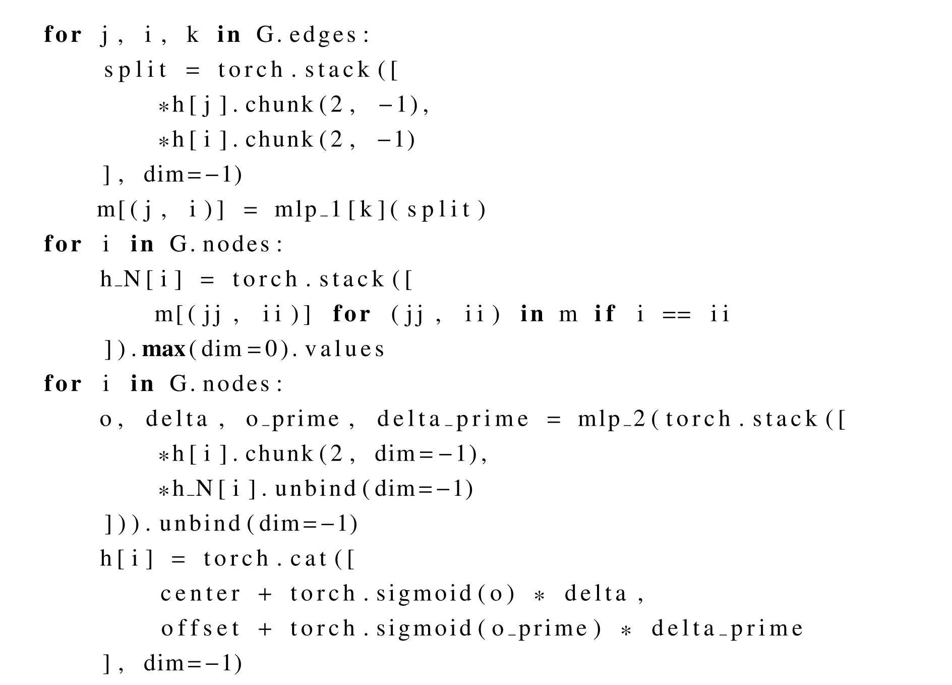
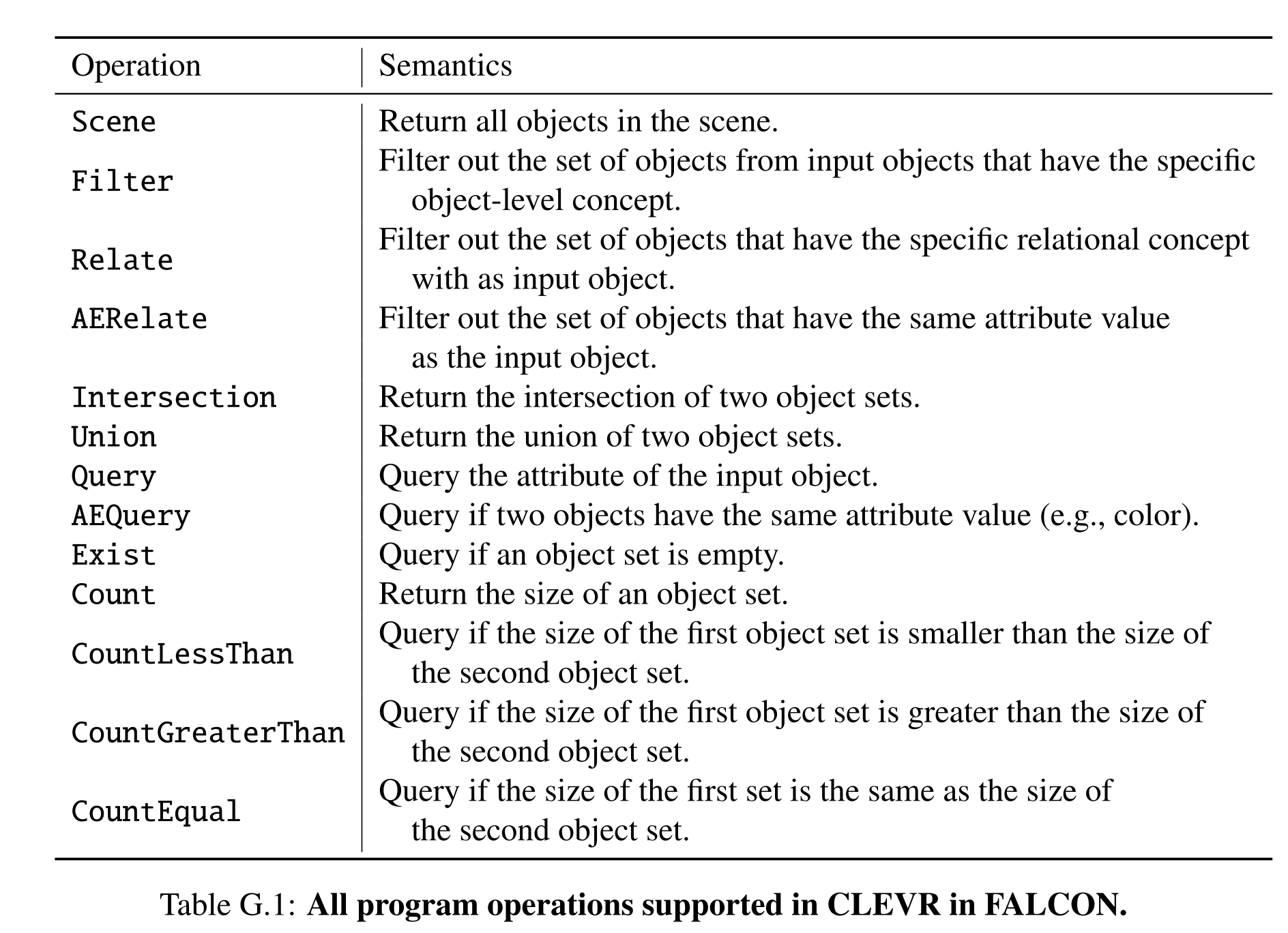
Table G.1: All program operations supported in CLEVR in FALCON.
Semantic parser
A sequence-to-sequence parser produces flattened operator–concept pairs that are reconstructed into trees. It is trained with program supervision on 10% of generated data. Descriptive-sentence programs extract the referenced object using known concepts, rather than requiring the new concept to identify itself; supplemental language yields concept relationships. Fast visual learning therefore does not imply unsupervised or zero-shot acquisition of the language parser.
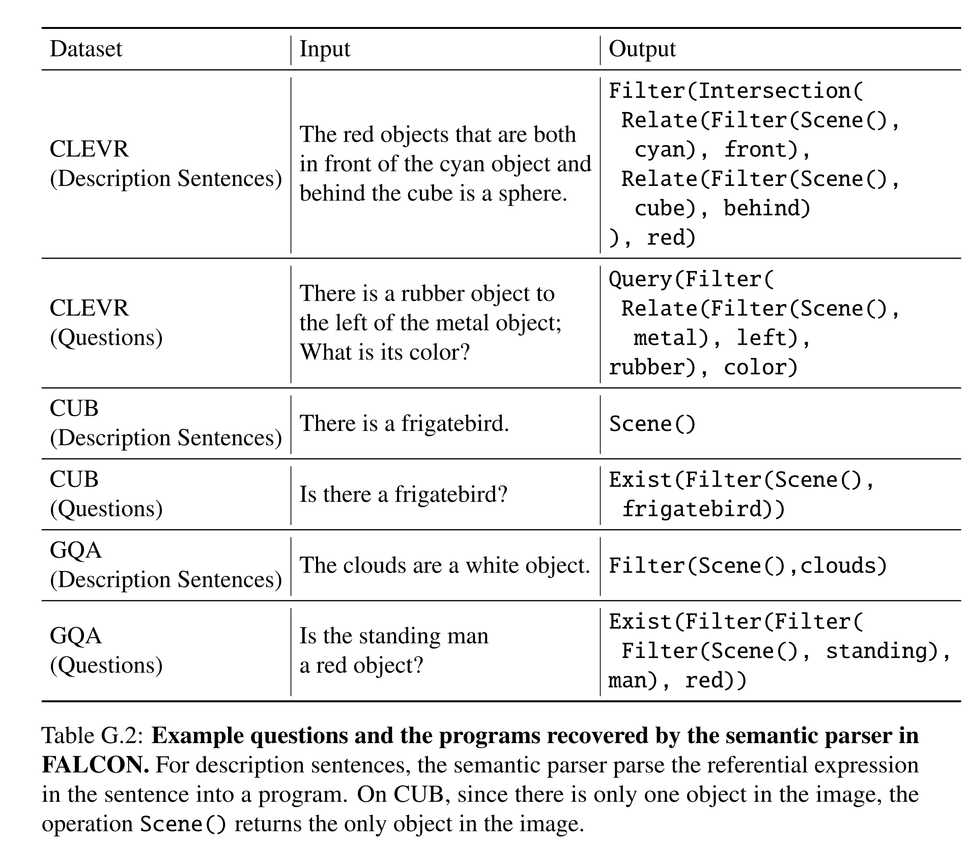
Table G.2: Example questions and the programs recovered by the semantic parser in FALCON. For description sentences, the semantic parser parse the referential expression in the sentence into a program. On CUB, since there is only one object in the image, the operation Scene() returns the only object in the image.
Neuro-Symbolic Progrm Execution
The executor retains NS-CL’s differentiable soft-set operations while replacing concept classification with the selected embedding-space score. Attribute equality is represented through learned relation concepts. This keeps the reasoning machinery shared across models, so changes to novel-concept inference can be evaluated through downstream answers.
Baseline Implementation
CNN+LSTM and MAC combine image features and task text directly. The appendix’s NSCL+LSTM encodes example vectors and sequences of related-concept embeddings and relations, rather than only raw supplemental sentences as the main description suggests. NSCL+GNN initializes from examples; for a single example without supplemental relations, it uses the average base-concept box size. That implemented initialization qualifies the main text’s claim that the baseline cannot handle this setting.
Training Details
Base training runs 50,000 iterations with batch size 10 and Adam at 10⁻⁴; meta-training runs 10,000 iterations with batch size one and learning rate 10⁻³. Validation occurs every 1,000 iterations, with learning-rate reduction after five unimproved evaluations. CLEVR uses an NS-CL-style curriculum. End-to-end baselines receive an unknown-word token for unseen concepts during both training and testing.
Experiment Details
All three datasets construct descriptions, supplemental relations, and test questions from annotations and templates. The following sections specify concept splits, question counts, continual ordering, biased examples, and the empirical relation between box geometry and entailment.
The CUB Dataset
CUB generates approximately 1,800 descriptions and 54,000 test-question pairs, with about 11,800 pairs for base pretraining. Supplemental related concepts are dropped independently with probability 0.2 during training. Continual learning orders concepts by taxonomy distance from the base set and freezes each inferred embedding for later reuse. Table G.4 gives 79.67% for box-based FALCON-G; with visual examples alone, Table G.5 gives 75.28%.
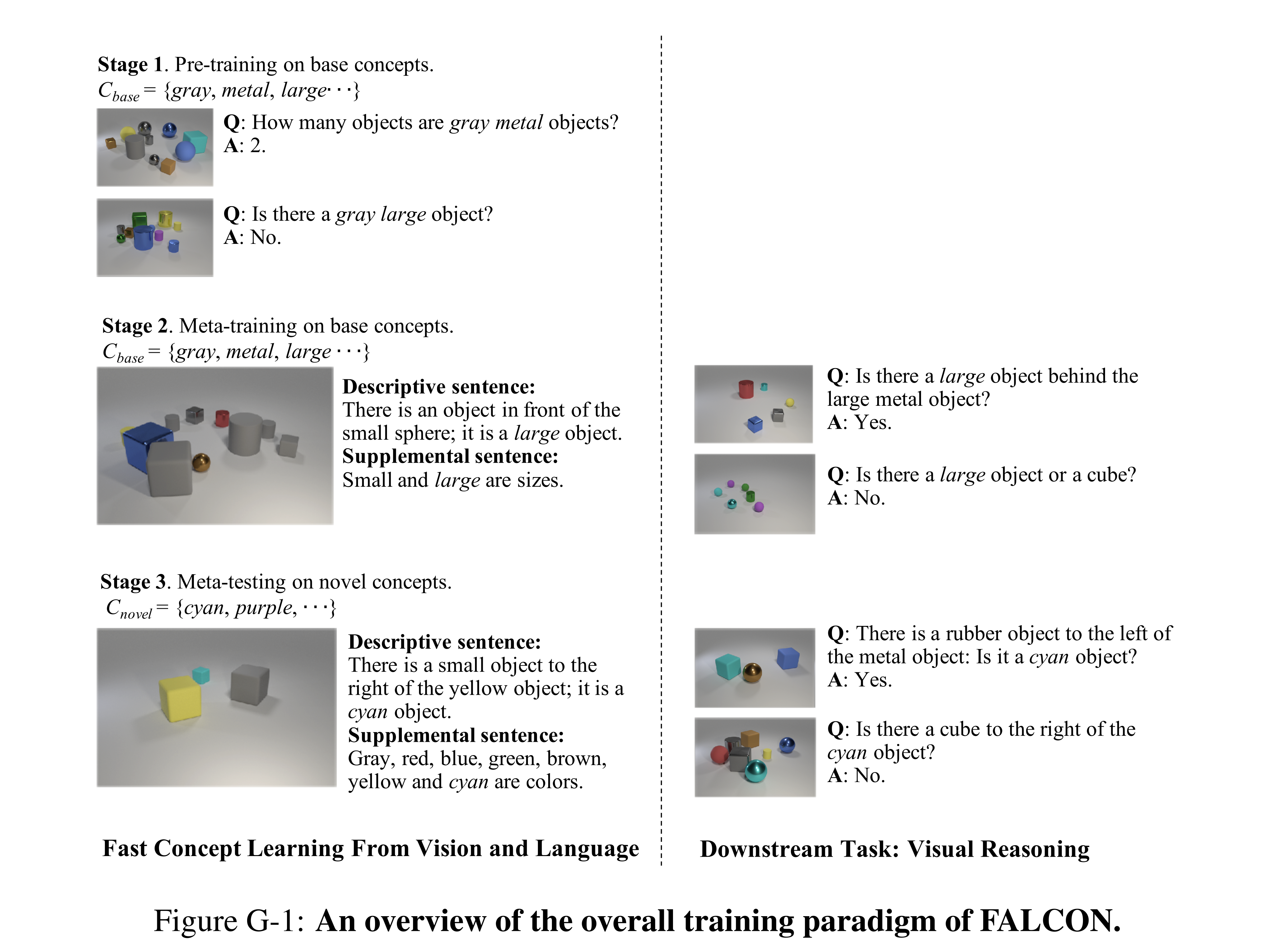
Figure G-1: An overview of the overall training paradigm of FALCON.
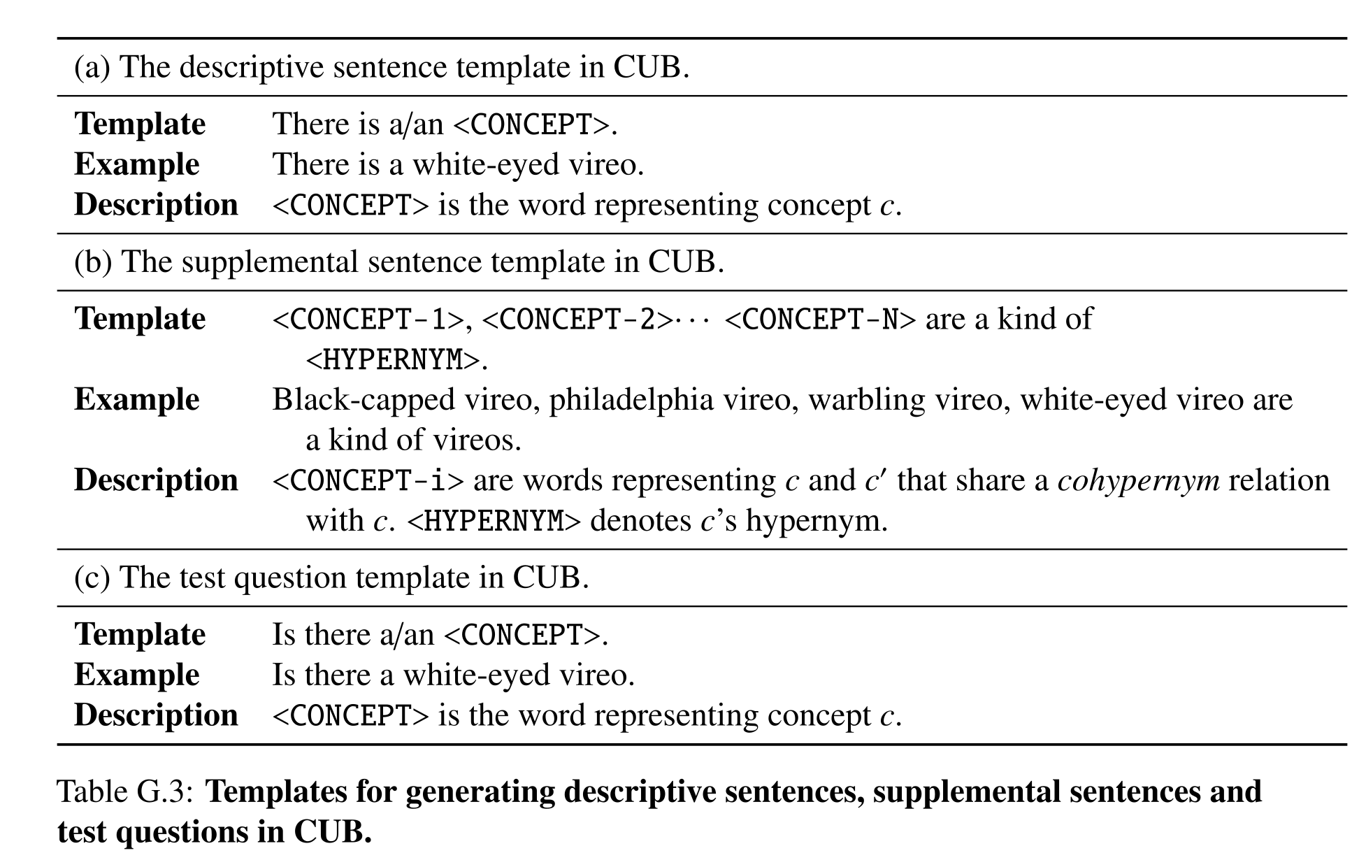
Table G.3: Templates for generating descriptive sentences, supplemental sentences and test questions in CUB.
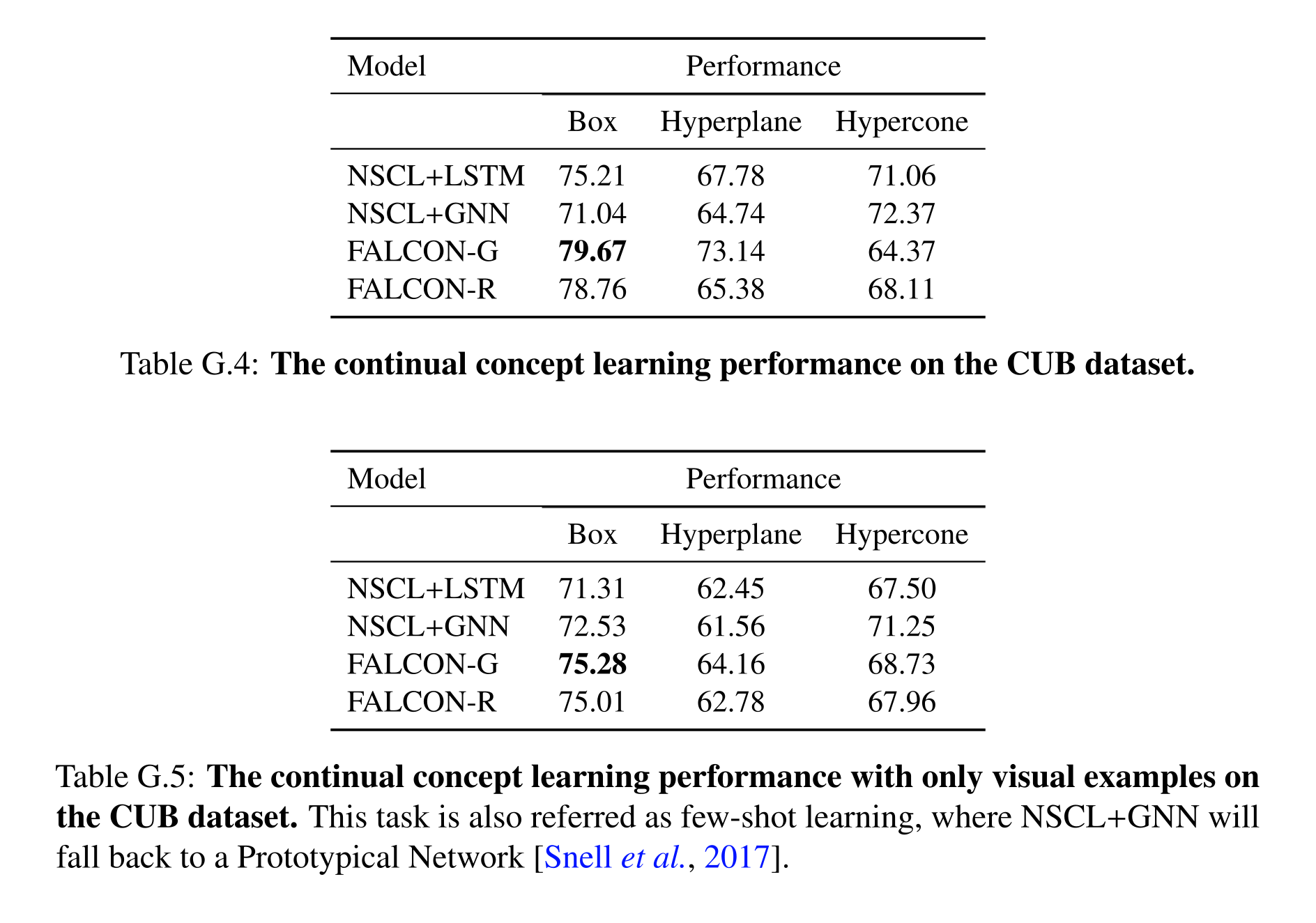
Table G.4: The continual concept learning performance on the CUB dataset.
Table G.5: The continual concept learning performance with only visual examples on the CUB dataset. This task is also referred as few-shot learning, where NSCL+GNN will fall back to a Prototypical Network [Snell et al., 2017].
The CLEVR Dataset.
CLEVR generates 7,500 descriptions, 225,000 downstream question pairs, and 402,000 pretraining questions. A test question contains one occurrence of the novel concept and may compose many base concepts. Biased examples deliberately conflate a color with a shape; supplemental information resolves which attribute the word denotes. Connecting the novel concept to known concepts sharing its attribute scores 88.40%, whereas representing the abstract attribute itself as a graph node scores 71.34%, motivating the former graph construction.
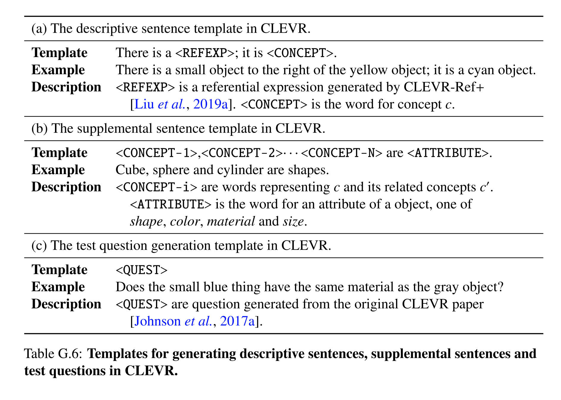
Table G.6: Templates for generating descriptive sentences, supplemental sentences and test questions in CLEVR.
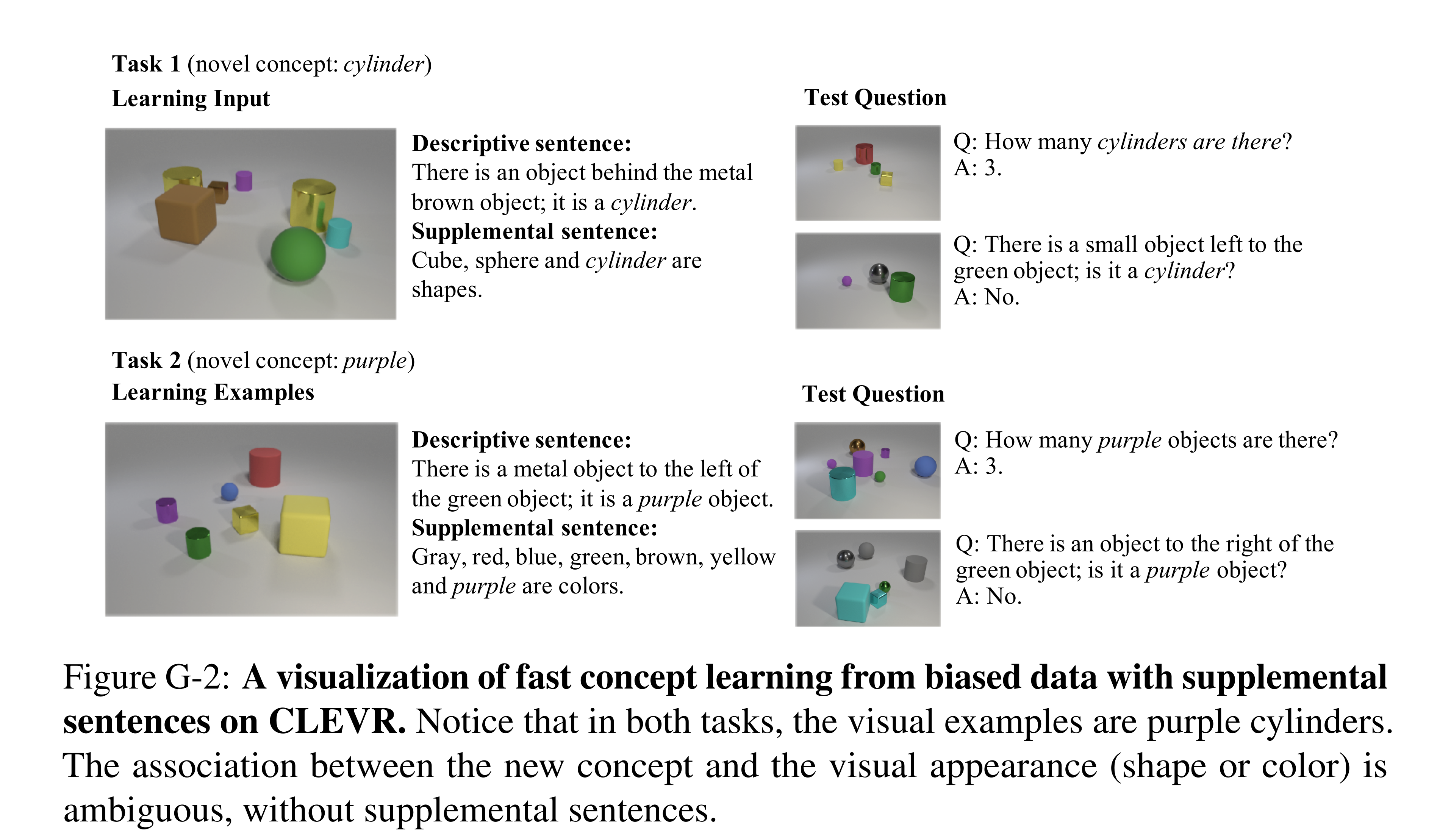
Figure G-2: A visualization of fast concept learning from biased data with supplemental sentences on CLEVR. Notice that in both tasks, the visual examples are purple cylinders. The association between the new concept and the visual appearance (shape or color) is ambiguous, without supplemental sentences.
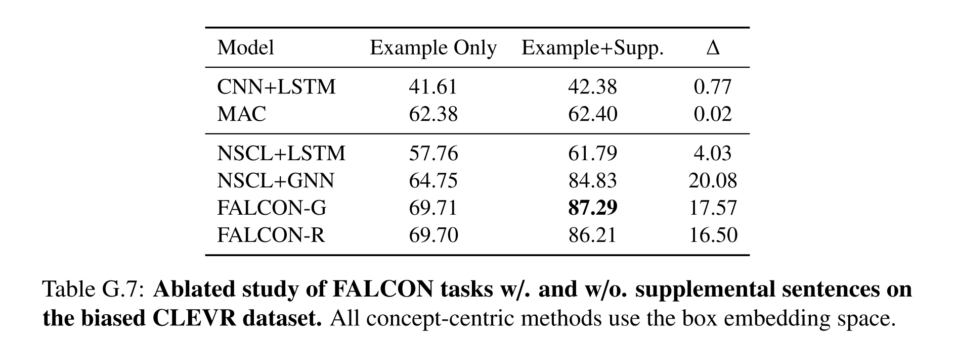
Table G.7: Ablated study of FALCON tasks w/. and w/o. supplemental sentences on the biased CLEVR dataset. All concept-centric methods use the box embedding space.
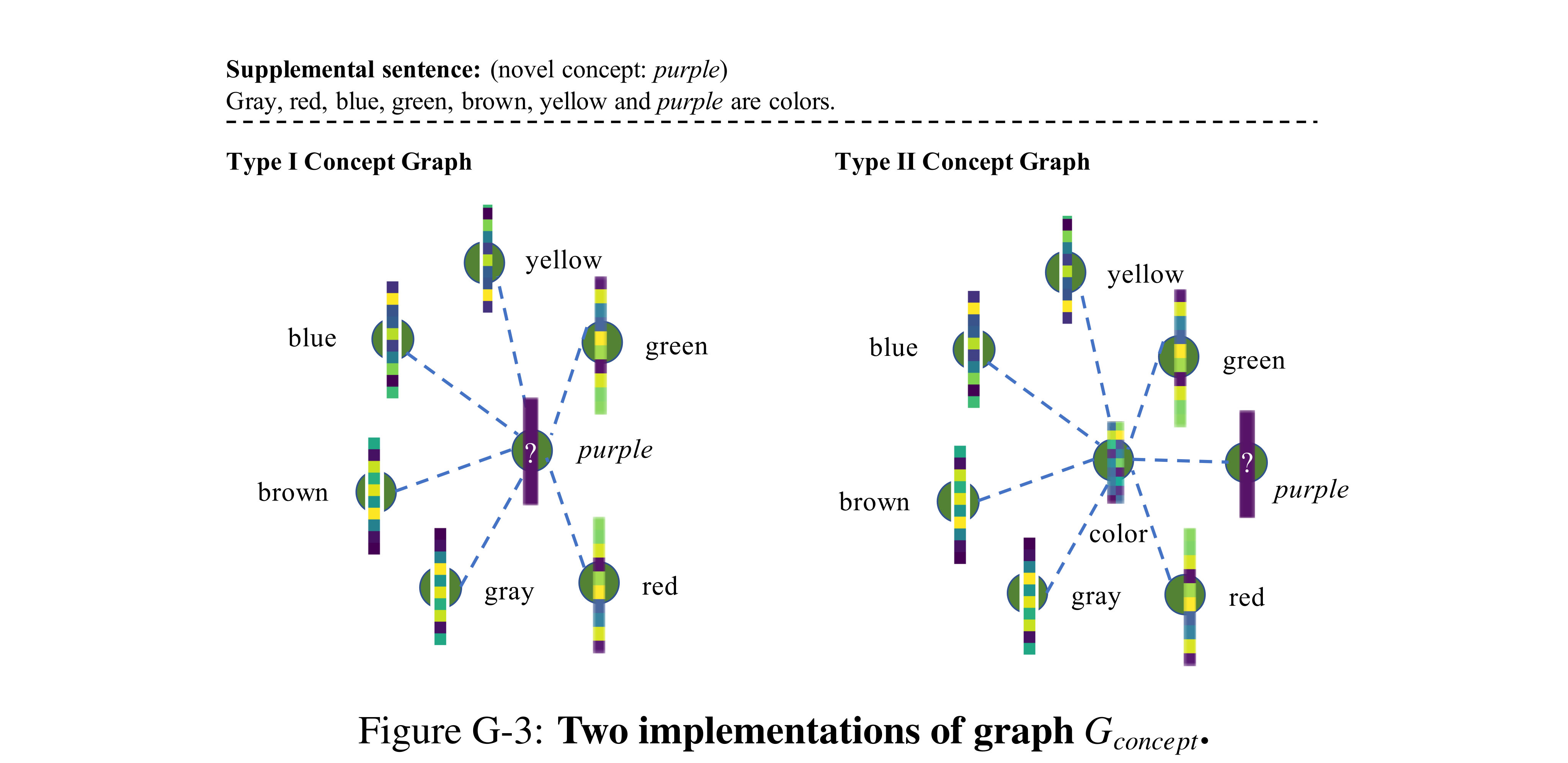
Figure G-3: Two implementations of graph Gconcept.
The GQA dataset
GQA uses pretrained Faster-RCNN object features and generated referential descriptions, shared-property statements, and binary test questions. Table G.9 reports FALCON-G’s 55.96% with supplemental information; without it, FALCON-R reaches 54.60%, just above MAC’s 54.45%, while G reaches 53.89%. The prose’s 117,000 total questions does not equal its listed 13,800/18,000/30,000 split counts, so the exact dataset total is ambiguous.
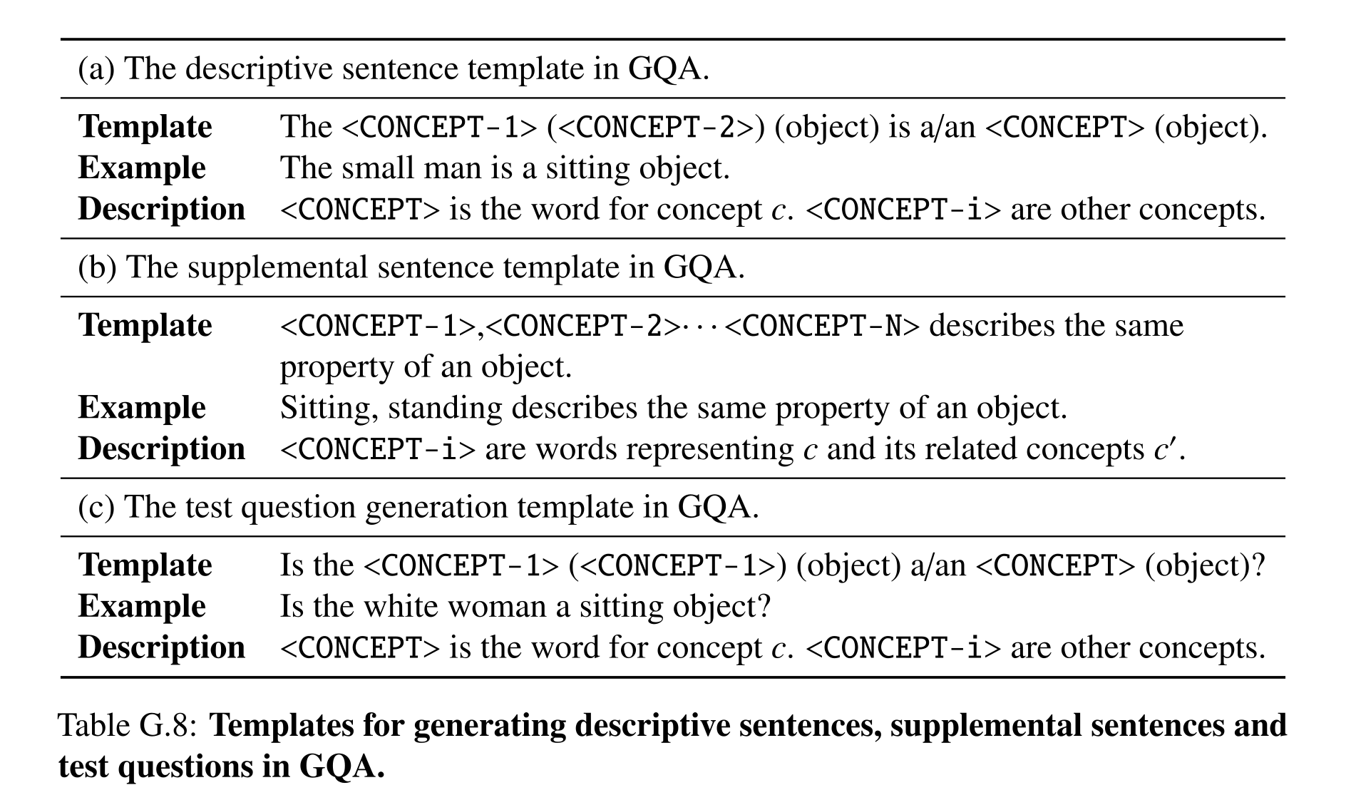
Table G.8: Templates for generating descriptive sentences, supplemental sentences and test questions in GQA.
The connections between the box embedding and our formulation
For entailment, the subclass box should lie inside the superclass box; the introductory containment sentence reverses these roles, while the later conditional-probability formula has the intended direction. Learned updates encourage but do not enforce such containment, and same-attribute relationships need not be entailments. On CUB concept-pair classification, box-based FALCON-G reaches ROC-AUC 0.855 versus 0.638 and 0.585 for hyperplanes and hypercones. The latter scores use symmetric similarities and are not naturally directed entailment models.
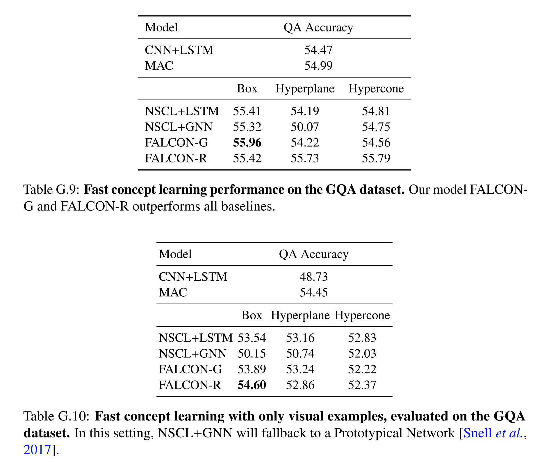
Table G.9: Fast concept learning performance on the GQA dataset. Our model FALCON- G and FALCON-R outperforms all baselines.
Table G.10: Fast concept learning with only visual examples, evaluated on the GQA dataset. In this setting, NSCL+GNN will fallback to a Prototypical Network [Snell et al., 2017].
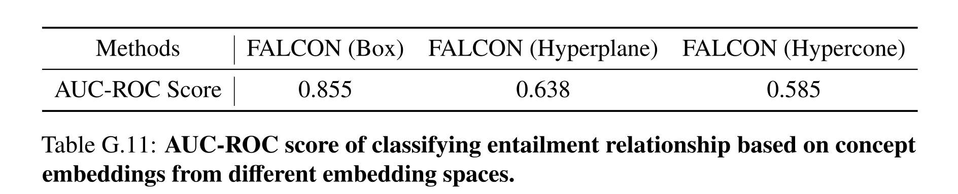
Table G.11: AUC-ROC score of classifying entailment relationship based on concept embeddings from different embedding spaces.
Ablation Details
Ablations vary the size of the base concept library and the amount of supplemental relation information. They test how much prior conceptual structure supports fast inference; changing the base split also changes the validation and test concept populations.
The Effect of the Number of Base Concepts
Reducing pretraining from 100 species/211 base concepts to 50 species/130 concepts lowers FALCON-G from 81.33% to 76.32%. It remains ahead of NSCL+GNN (75.21%) and MAC (65.16%) in the smaller split. Because the test concepts also change, the difference is evidence for the value of richer base training under these protocols, not an isolated causal estimate of library size.
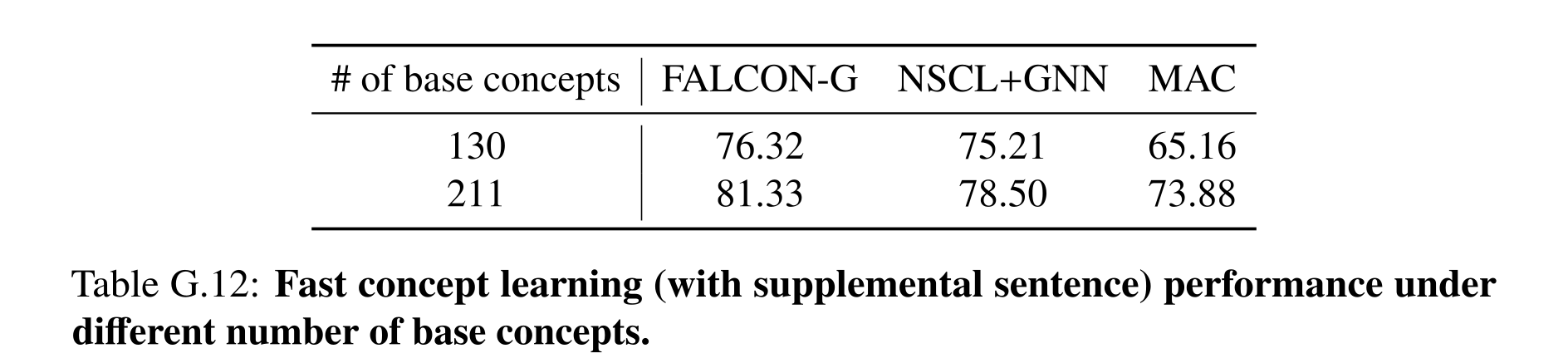
Table G.12: Fast concept learning (with supplemental sentence) performance under different number of base concepts.
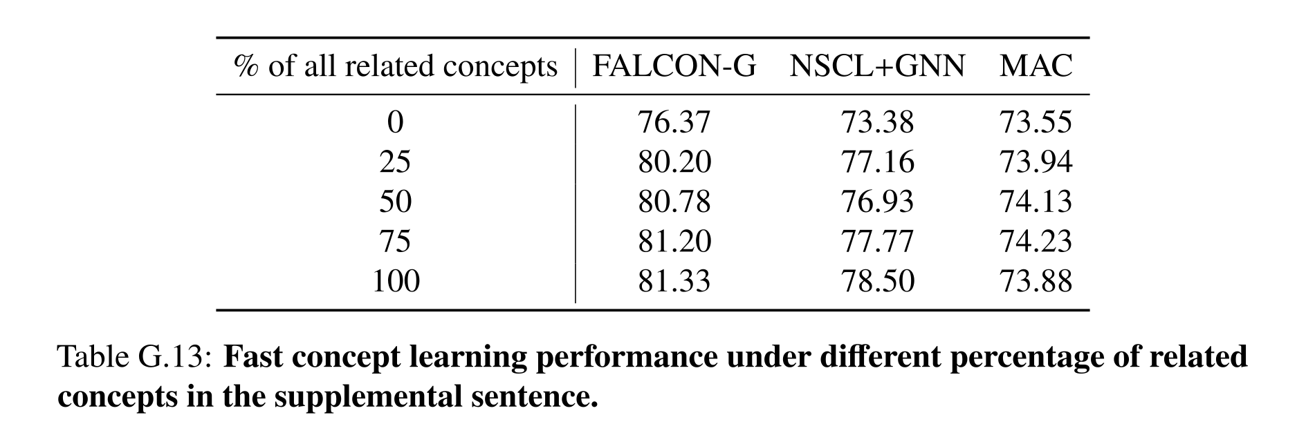
Table G.13: Fast concept learning performance under different percentage of related concepts in the supplemental sentence.
The Effect of The Number of Related Concepts in Supplemental Sentences
With 0%, 25%, 50%, 75%, and 100% of related concepts supplied, FALCON-G scores 76.37%, 80.20%, 80.78%, 81.20%, and 81.33%. Most of its gain arrives with the first quarter of relations. The other models fluctuate rather than improving strictly monotonically, so the result supports generally useful partial information without guaranteeing that every additional relation helps.
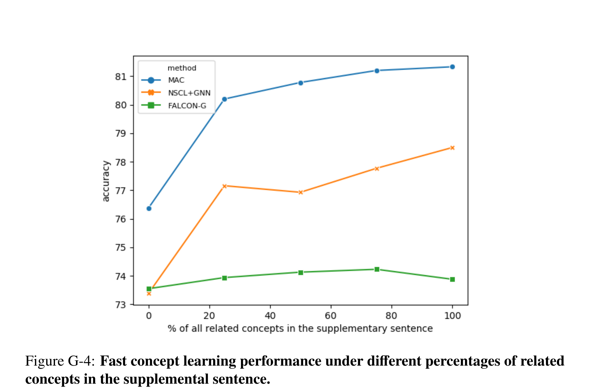
Figure G-4: Fast concept learning performance under different percentages of related concepts in the supplemental sentence.
Failure Mode Details
Detection, parsing, and grounding errors can corrupt either the selected learning example or downstream reasoning. A correct answer can survive an incorrect intermediate representation, so answer accuracy alone does not establish semantic correctness of the learned program or concept.
Failure mode in detection module
Small or occluded objects may be missed, and shadows or merged regions may create false detections. Missing the referenced object can teach the new concept from the wrong example; unrelated false positives can leave the selected object and final answer unchanged. Figures G.5 shows both outcomes rather than treating every detector error as a question-answering failure.
Failure mode in semantic parser
Heuristics remove invalid subprograms when parser outputs are syntactically infeasible. Syntactically valid but semantically wrong programs are executed unchanged and can produce either wrong answers or accidentally correct ones when descriptions are redundant. No semantic-error recovery is implemented; visual feedback through reinforcement learning is proposed as future work.
Failure mode in concept learning module
An overly broad relation can select the wrong training object, while an overly narrow novel concept can exclude a valid test object. Both base and newly learned concepts can suffer imperfect grounding. Subsequent operations may expose or conceal the mistake, which motivates inspecting the example selection and execution trace in addition to the final answer.
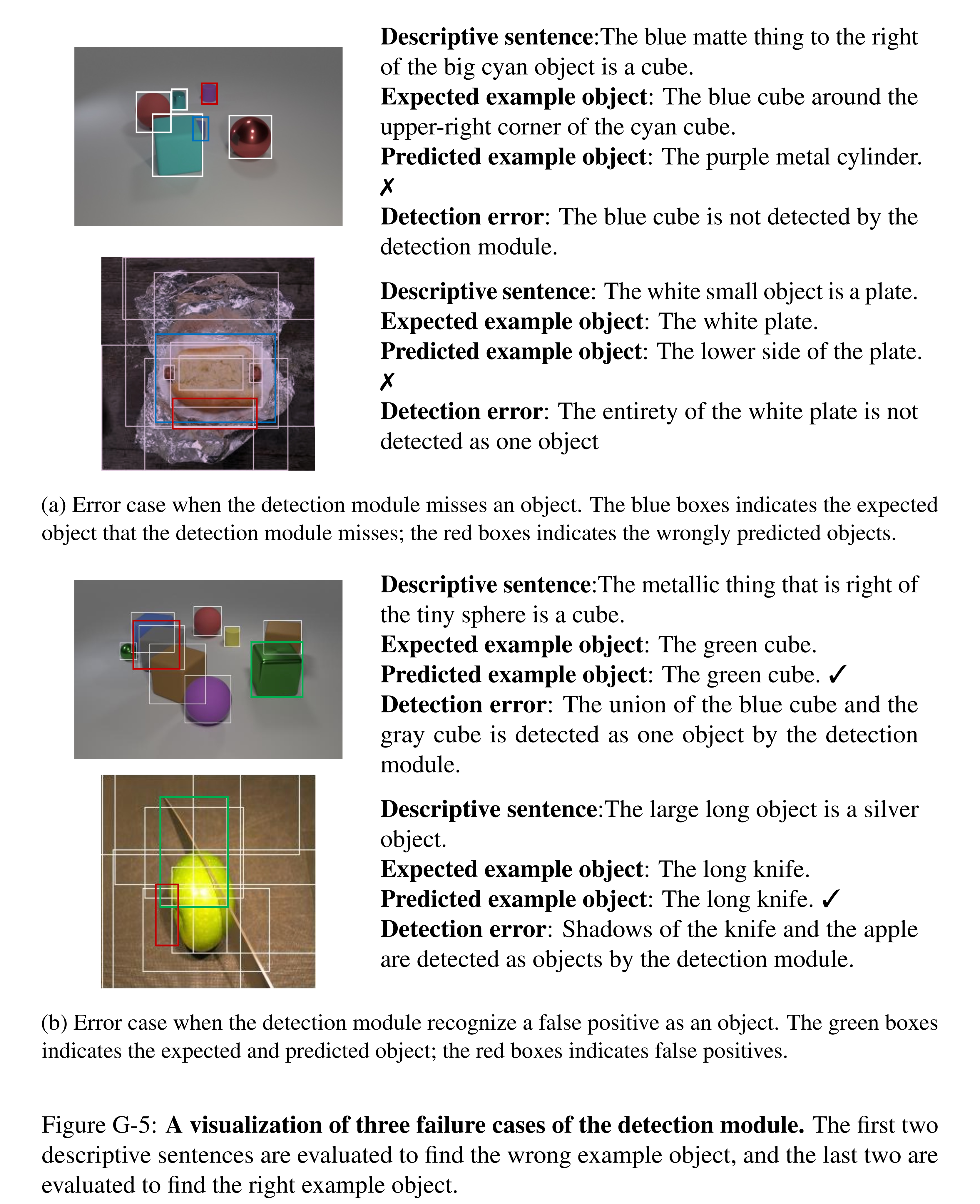
Figure G-5: A visualization of three failure cases of the detection module. The first two descriptive sentences are evaluated to find the wrong example object, and the last two are evaluated to find the right example object.
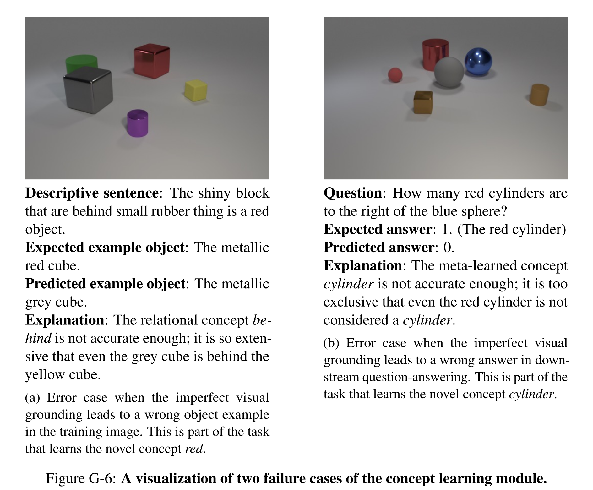
Figure G-6: A visualization of two failure cases of the concept learning module.

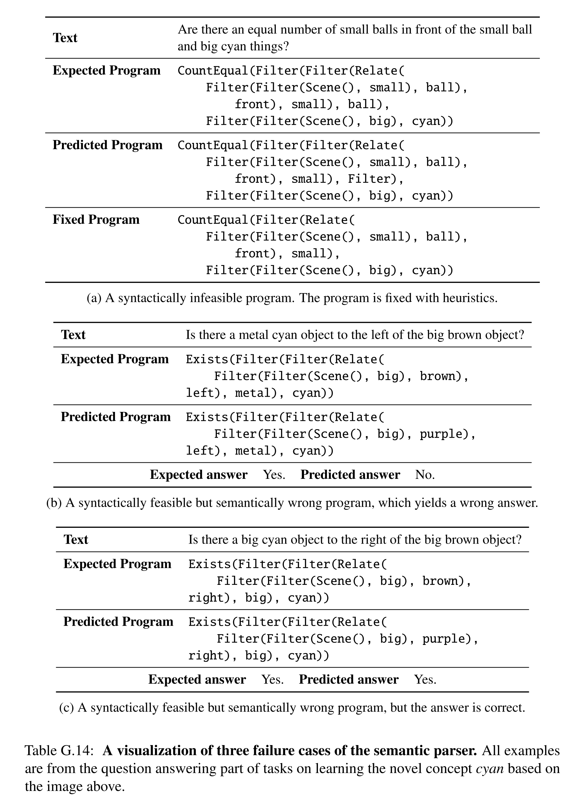
Table G.14: A visualization of three failure cases of the semantic parser. All examples are from the question answering part of tasks on learning the novel concept cyan based on the image above.
Appendix for Concept Learning Across Domains and Modalities
The appendix formalizes the differentiable executor, reports limited multi-seed results, defines the generated transfer tasks, and summarizes the implementation and training setup. It also notes the possibility of harmful biases inherited from the LLM interpreter.
LEFT
LEFT’s operator definitions specify how soft entity selections and predicate tensors compose. The broader-impact discussion concerns the pretrained interpreter’s outputs, which remain outside direct control even when its prompts contain only generic logic examples.
Function definitions
Table H.1 gives the exact quantifier, Boolean, selection, counting, comparison, and output operations. A concrete soft-selected entity is contracted with predicate scores by a dot product; textual arguments may use generative outputs. Unary and binary predicate networks extend to higher arities. Although signatures use Boolean or integer labels, execution uses relaxed scores and expected counts during differentiable inference.
Broader impact
The pretrained LLM may generate harmful biases that the generic first-order-logic prompts do not eliminate. The authors propose documenting this concern with the code release; the appendix does not present a bias evaluation or a mitigation guarantee.
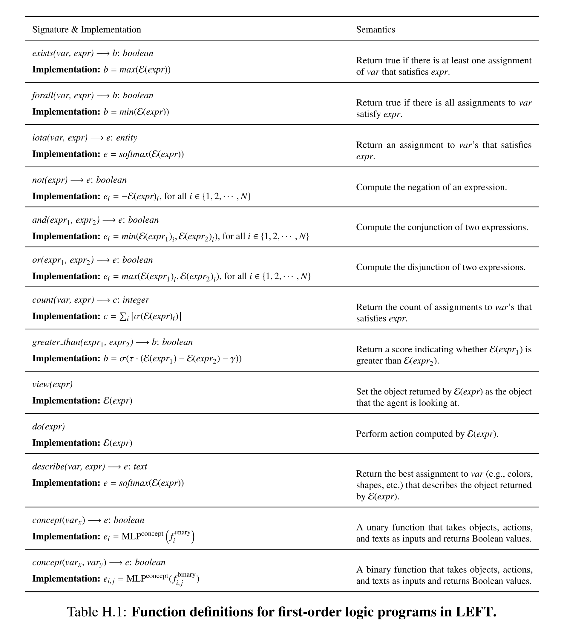
Table H.1: Function definitions for first-order logic programs in LEFT.
Experiments
Additional experiments report three-seed standard errors for selected CLEVR settings and specify the templates used to generate the three zero-shot reasoning tasks. These details establish the scope of the evidence and distinguish the tasks from unrestricted natural-language or visual reasoning.
Error bars
Across three random seeds, LEFT scores 0.942 ± 0.008 on 10% CLEVR and 0.996 ± 0.001 on full CLEVR. CLEVR-Humans scores are 0.780 ± 0.003 on executable queries and 0.694 ± 0.001 on all queries. The reported uncertainty is standard error, not standard deviation or a confidence interval; equivalent multi-seed results are not supplied here for every domain or transfer task.
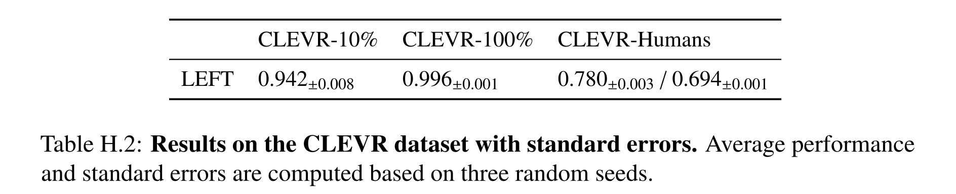
Table H.2: Results on the CLEVR dataset with standard errors. Average performance and standard errors are computed based on three random seeds.
Transfer task construction
CLEVR-Ref uses four referring-expression templates with known object attributes and relations, excluding ordinal-number expressions. Puzzles specify four ambiguous object descriptions plus three relations, with a unique global solution. RPM prompts describe eight cells of a 3×3 grid in text and vary row/column progression attributes; the model infers the ninth description and searches the image for a matching object. These tasks introduce new compositions of trained concepts.
Model
The implementation separates GPT-3.5 interpretation, predicate initialization, modality encoders, and recursive differentiable execution. Dataset splits and several optimization choices follow existing benchmark and baseline implementations.
Implementation details
The interpreter emits first-order logic, and a domain initializer creates each concept embedding according to the parsed predicate arity. Grounding modules then extract entity and relation features, and the shared executor combines their scores. This modular implementation makes the common reasoning interface explicit while leaving the representation of each input modality domain-specific.
Training details
Training uses the official CLEVR, ReferIt3D, HumanMotionQA, and CLIPort splits, concept embeddings of dimension 128, and learning rates drawn from the corresponding neuro-symbolic baselines. The appendix delegates complete hyperparameters to released code; it does not supply one universal optimization schedule for all domains.
Appendix for Visual Lexicon Learning
The appendix defines both domain-specific languages and their differentiable implementations, illustrates expected execution, states its assumptions, and details the generalization splits. It also reveals important engineering restrictions: pretrained object detection, hand-selected visual lexical templates, special handling of coordination, and exclusion of ambiguous language.
Domain Specific Languages and Neuro-Symbolic Reasoning
Each domain supplies typed, manually designed operations implemented with tensors so their outputs can receive gradients. Visual programs operate on soft object sets and concepts; navigation programs operate on probabilistic action strings. The lexical forms are learned within these supplied representational choices.
Visual Reasoning DSL
The visual DSL has six types and eight operations. Pretrained Mask R-CNN boxes and ResNet-34 features represent objects; product intersection and probabilistic union replace minimum/maximum to support expected execution. The explicit unique operator is removed, with uniqueness handled inside relevant operations. Ten hand-selected lexical templates, an empty entry, three word-specific concept representations, and special conjunction/disjunction rules constrain learning. Object-set alternatives are merged using softmax-weighted results and log-sum-exp weights. The printed type table has an unfinished attribute description, and the existence description says “empty”; these are source defects rather than additional model semantics.
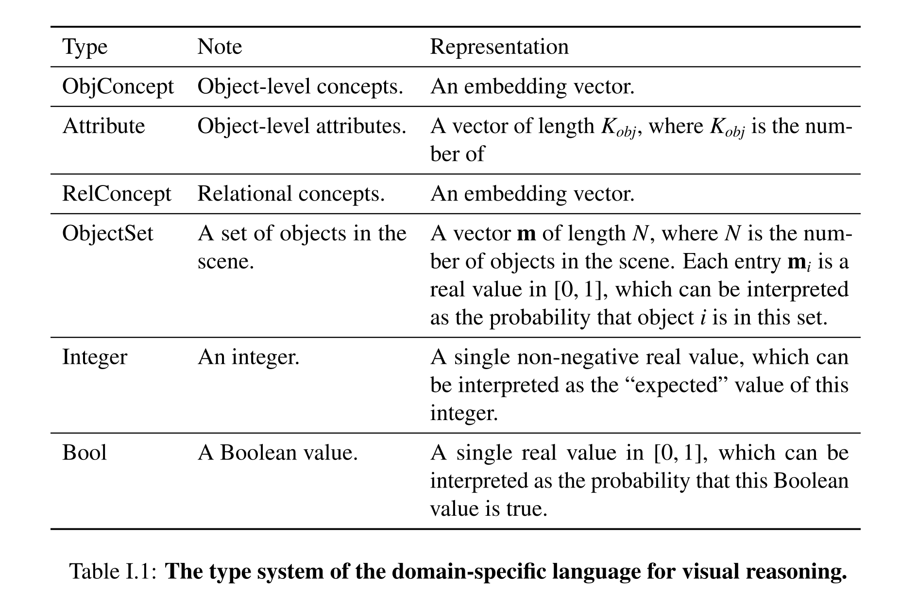
Table I.1: The type system of the domain-specific language for visual reasoning.
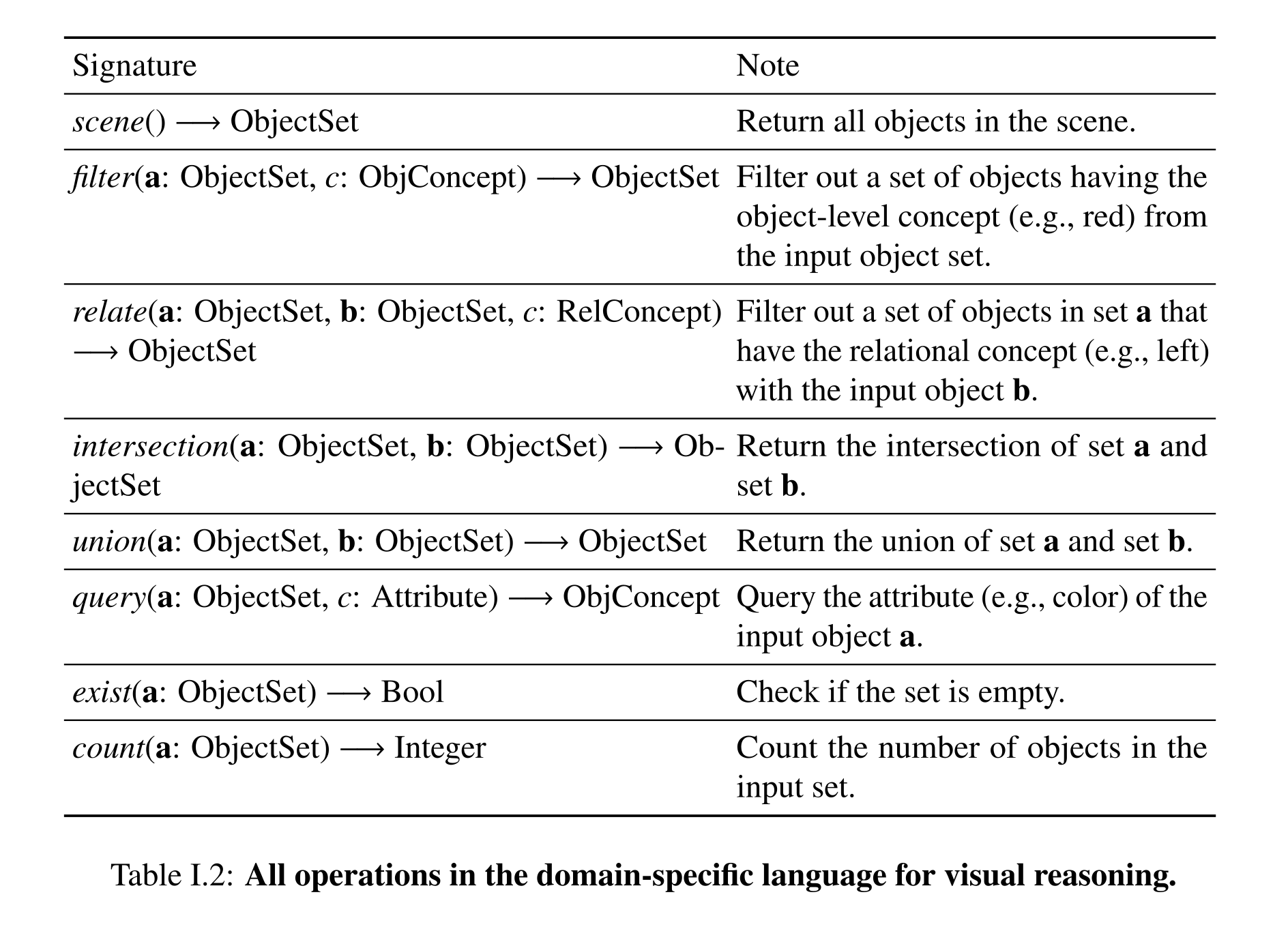
Table I.2: All operations in the domain-specific language for visual reasoning.
Equation

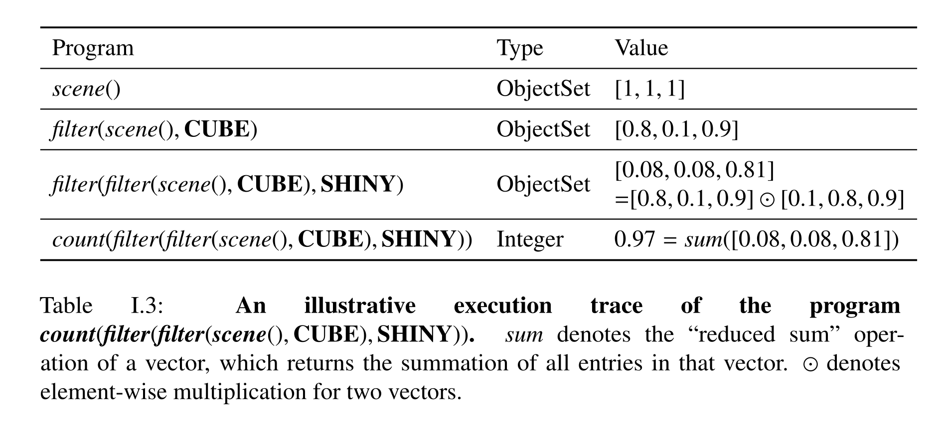
Table I.3: An illustrative execution trace of the program count(filter(filter(scene(), CUBE), SHINY)). sum denotes the “reduced sum” oper- ation of a vector, which returns the summation of all entries in that vector. ⊙denotes element-wise multiplication for two vectors.
Equations



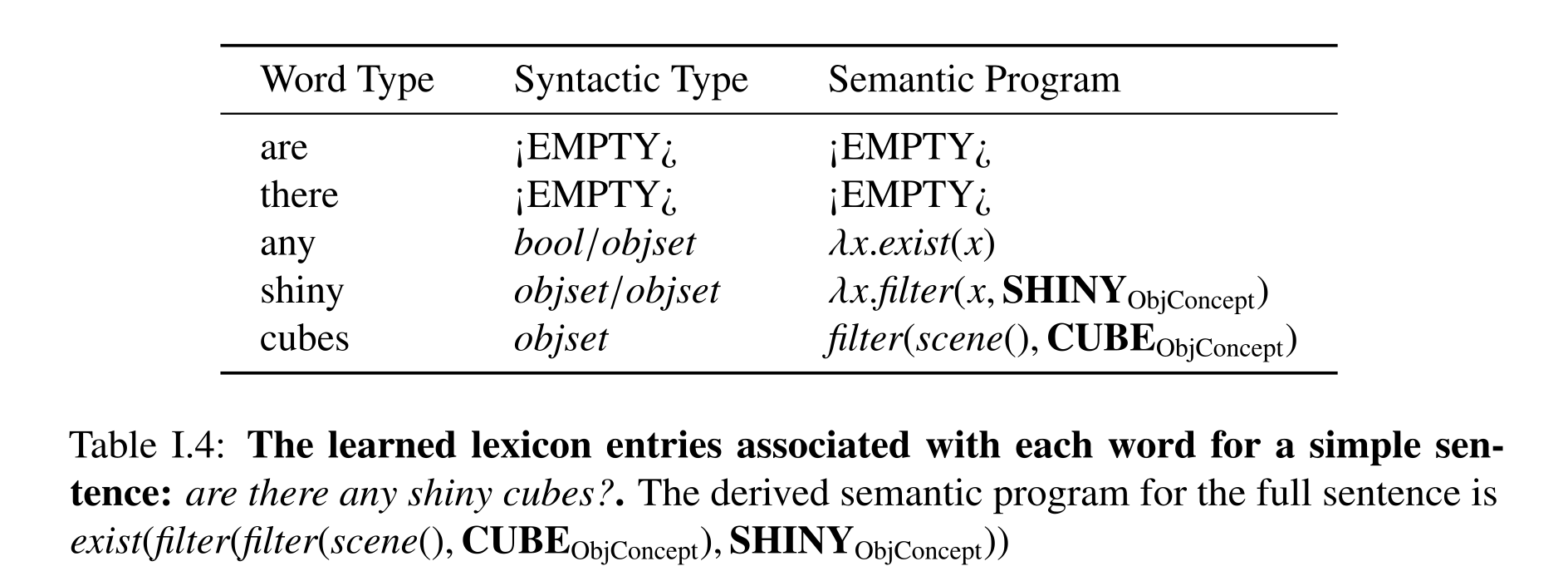
Table I.4: The learned lexicon entries associated with each word for a simple sen- tence: are there any shiny cubes?. The derived semantic program for the full sentence is exist(filter(filter(scene(), CUBEObjConcept), SHINYObjConcept))
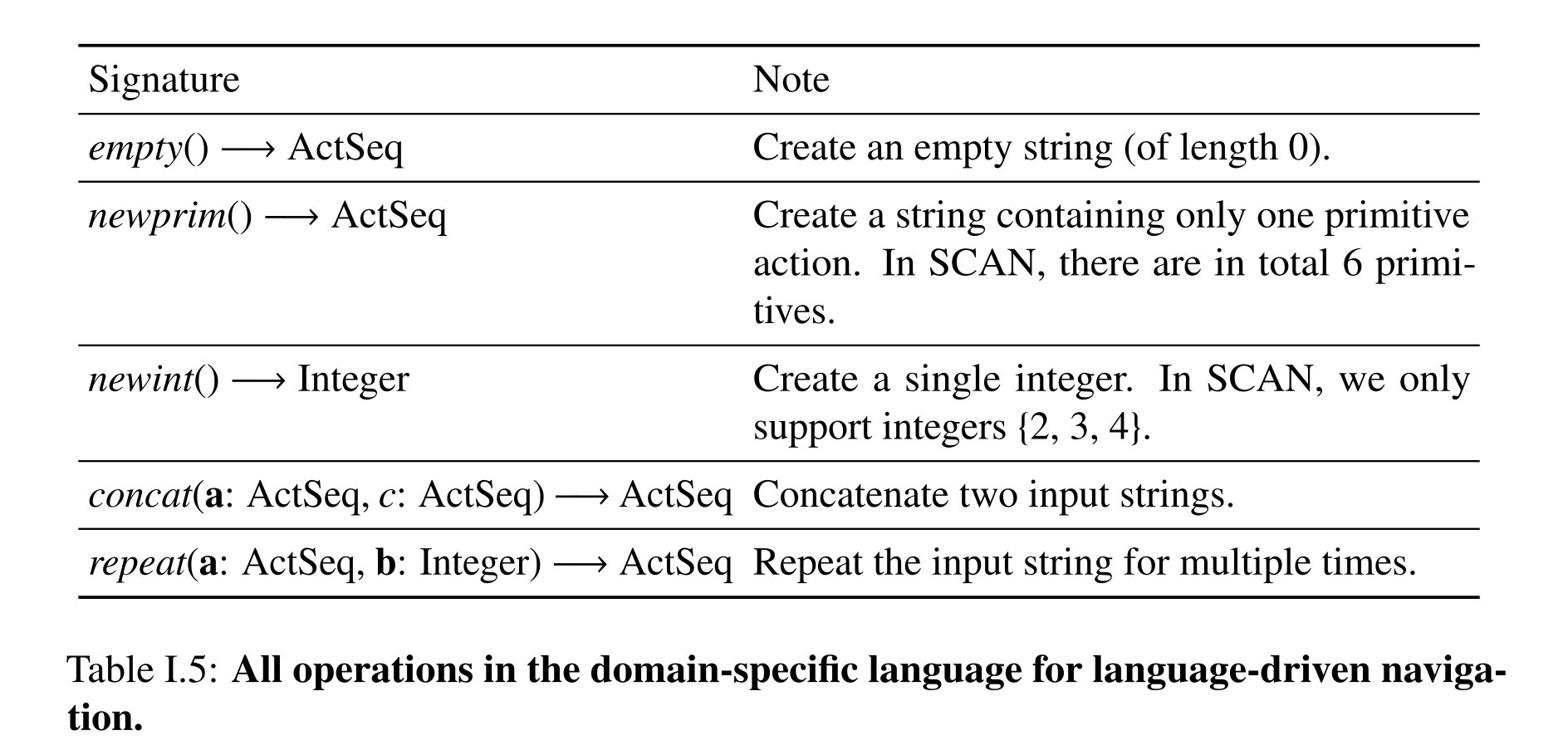
Table I.5: All operations in the domain-specific language for language-driven naviga- tion.
Language-Driven Navigation DSL
Navigation uses empty strings, primitive actions, small integer constants, concatenation, and repetition. A probabilistic string stores a length distribution and token distributions conditional on length; concatenation sums over length partitions, and expected execution merges these representations. Candidate programs have at most three operations, two arguments, one function-valued argument, and no integer-valued argument. Restricting syntactic categories to six patterns, including distinct S and V types, yields 178 candidates per word and helps disambiguate connective scope.
Equations



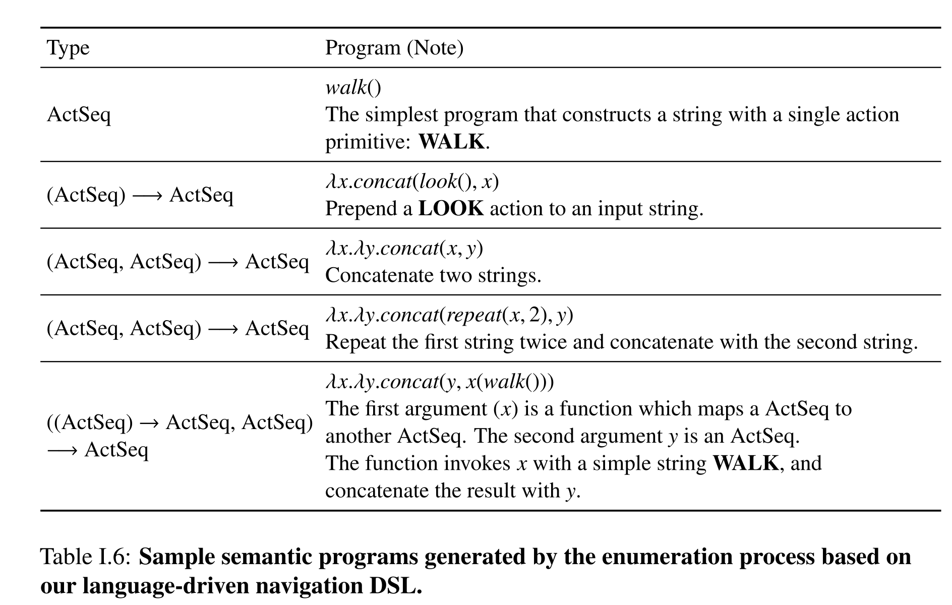
Table I.6: Sample semantic programs generated by the enumeration process based on our language-driven navigation DSL.
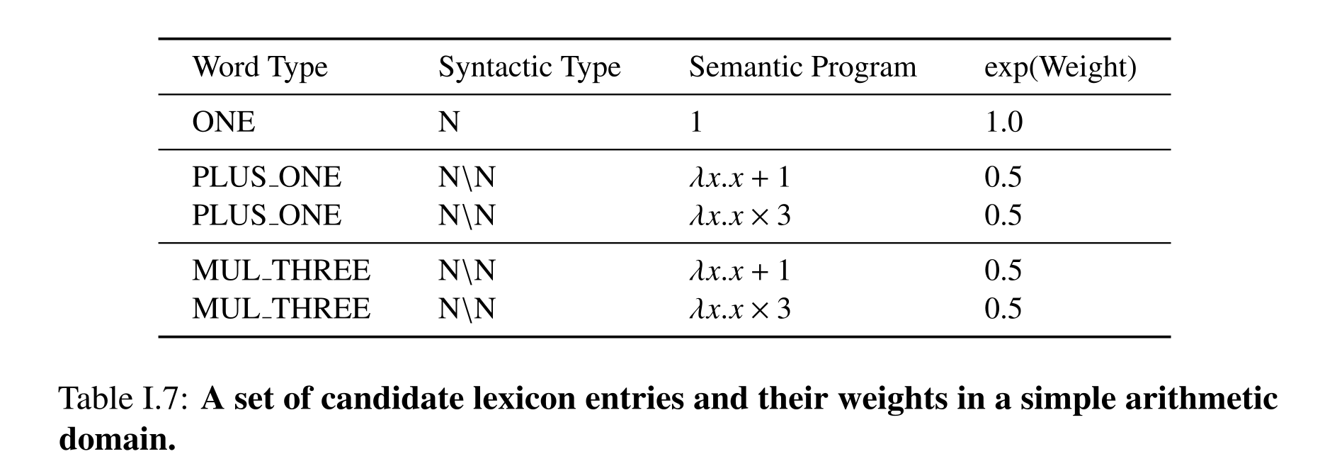
Table I.7: A set of candidate lexicon entries and their weights in a simple arithmetic domain.
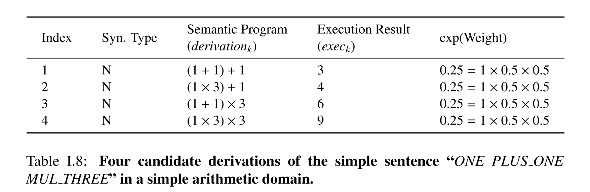
Table I.8: Four candidate derivations of the simple sentence “ONE PLUS ONE MUL THREE” in a simple arithmetic domain.
Delve Into Expected Execution
Expected execution replaces alternative grounded subprograms with their weighted result before composing larger spans. The arithmetic example demonstrates preservation of a mean, and the formal argument identifies the operator and structural assumptions needed for exactness and tractable storage.
CKY-E2 In An Arithmetic Domain
Four equally weighted arithmetic derivations yield 3, 4, 6, and 9, averaging 5.5. Merging the first constituent’s alternatives into 2.5 leaves only two later computations, 3.5 and 7.5, with the same mean. This example explains local compression; despite its mention of an L2 loss, preserving the mean alone does not preserve expected squared loss, which also depends on variance.
Equation

Formal Properties of CKY-E2
The proof factors derivation weights across adjacent constituents and assumes composition satisfies E[f(a,b)] = f(E[a],E[b]). Addition and independent multilinear products qualify; minimum, maximum, and general nonlinear transformations do not. Under a restricted grammar with one primitive type and bounded functor arity, each span retains at most 1 + N₁ + 2N₂ alternatives. This establishes polynomial storage in that setting; it is not an unrestricted complexity or exactness theorem for arbitrary program languages.
Equations



Connection with Other Parsing Models
Parsing can be viewed as synchronously constructing a syntax tree and a meaning program, with grounded answers providing distant supervision. CKY-E2 shares chart decomposition with sum-product parsing but stores expected executable values instead of the full distribution over possible programs. This compression is the source of efficiency and also limits what uncertainty about meanings is retained.
Experimental Setup And Analysis
The experimental protocols restrict the language to match the one-entry-per-word assumption and explicitly withhold particular compositions or output lengths. The analysis separates parsing failures from grounding failures and notes that a wrong program can still produce the correct answer.
Visual Reasoning: CLEVR
CLEVR retains 208 templates after removing coreference, same-attribute, and number-comparison questions, then regenerates the original number of question examples. Purple, right, and count training uses only short occurrences; appendix thresholds are 7, 12, and 9 tokens including punctuation, versus 6, 11, and 8 in the chapter. Depth testing moves from zero/one-hop to two-hop references. Baseline sequence parsers score 70.8% program accuracy on count and 1.7% on depth, while answer accuracy can remain higher through accidental agreement. The right-split parser discussion also conflicts with NS-VQA’s higher table accuracy, so these diagnostics should not be treated as a fully reconciled quantitative attribution.
Language-Driven Navigation: SCAN
SCAN’s simple split trains on 80% of generated pairs; the reduced-data variant samples 10% of that training set uniformly by input length. Jump appears only in isolation during training, around-right never appears, and length transfer trains on outputs of at most 22 actions before testing up to 48. Evaluation uses exact sequence matches. The appendix notes that GECA augmentation can generate examples belonging to the test set, especially for compositional splits, which qualifies direct comparisons of data exposure.
Appendix for Manipulation Mechanisms
This appendix specifies the mechanism planner, geometric samplers, constrained training/test distributions and a two-task physical deployment. Its details narrow the scope of the chapter’s broad generalization claims.
Method Detail
The implementation uses symbolic macro search followed by geometry-based sampling and simulated execution. Briefly dynamic effects are allowed between stable configurations; individual controllers remain position-based.
Planning Algorithm
Algorithm 13 enumerates symbolic sequences containing primitives and mechanisms. It samples continuous parameters, checks preconditions, simulates operators and accepts a sequence only when the goal is reached. Primitive steps originating inside a mechanism use its specialized sampler; others use the generic sampler.
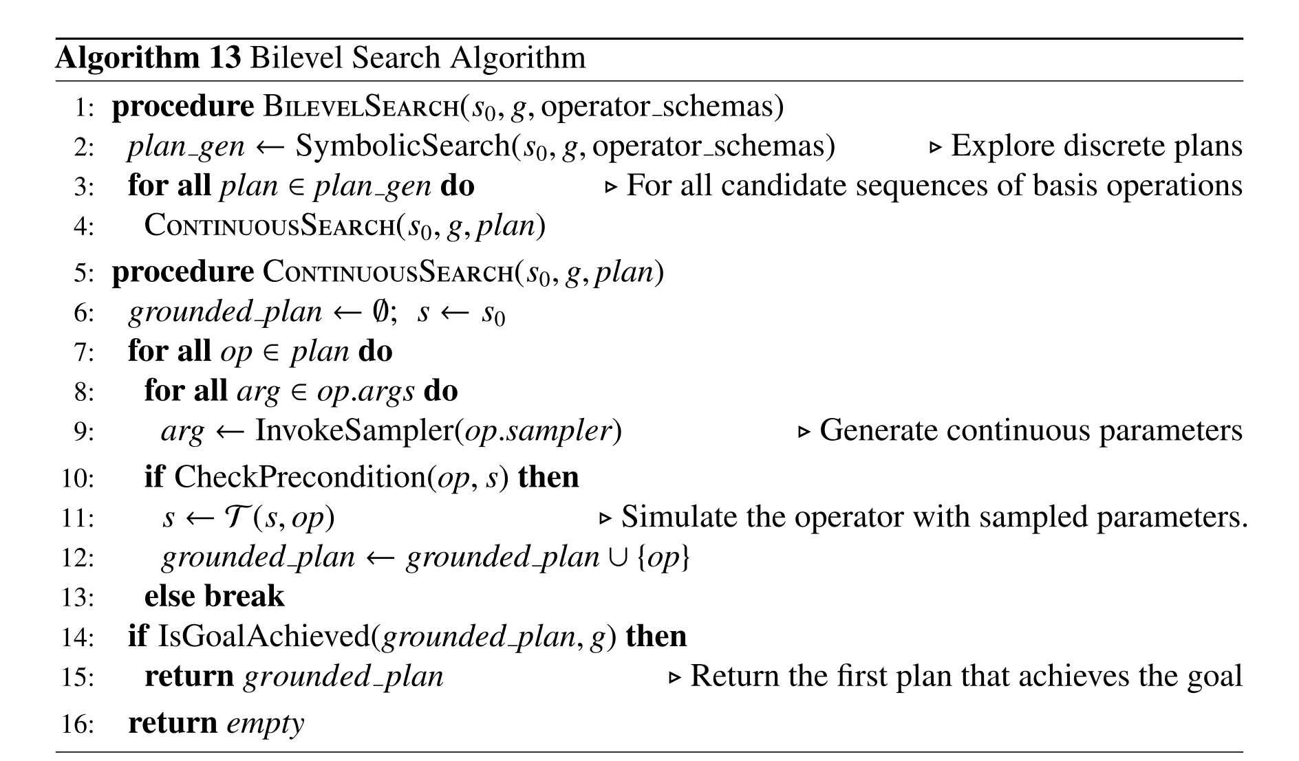
Briefly Dynamic Manipulation
Objects may slide after placement, change support poses or interact through nonrigid attachments before settling. These examples relax quasi-static assumptions while still requiring stable endpoints and a simulator accurate enough to predict them.
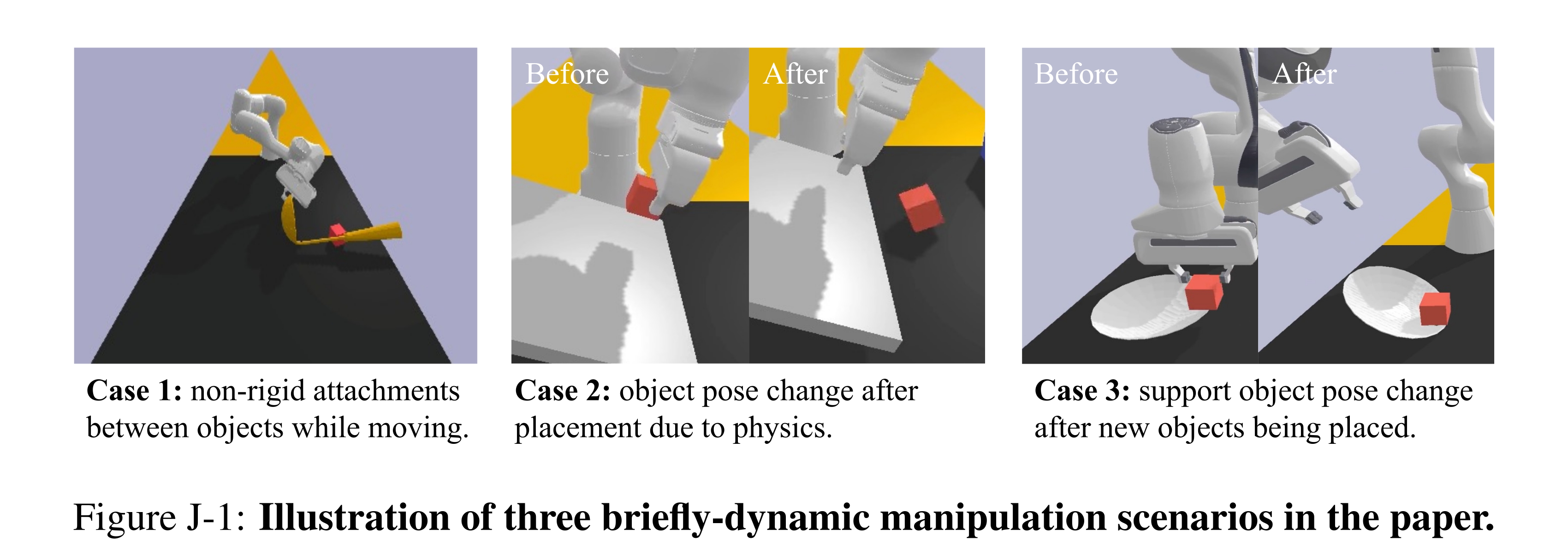
Figure J-1: Illustration of three briefly-dynamic manipulation scenarios in the paper.
Basis Operations
Basis actions either preserve the contact graph or change one contact mode. The move-with-contact schema describes the held tool, contacted target, support, contact geometry and joint trajectory; execution updates robot/tool/target poses. Preconditions encode holding, support and feasible contact/motion.
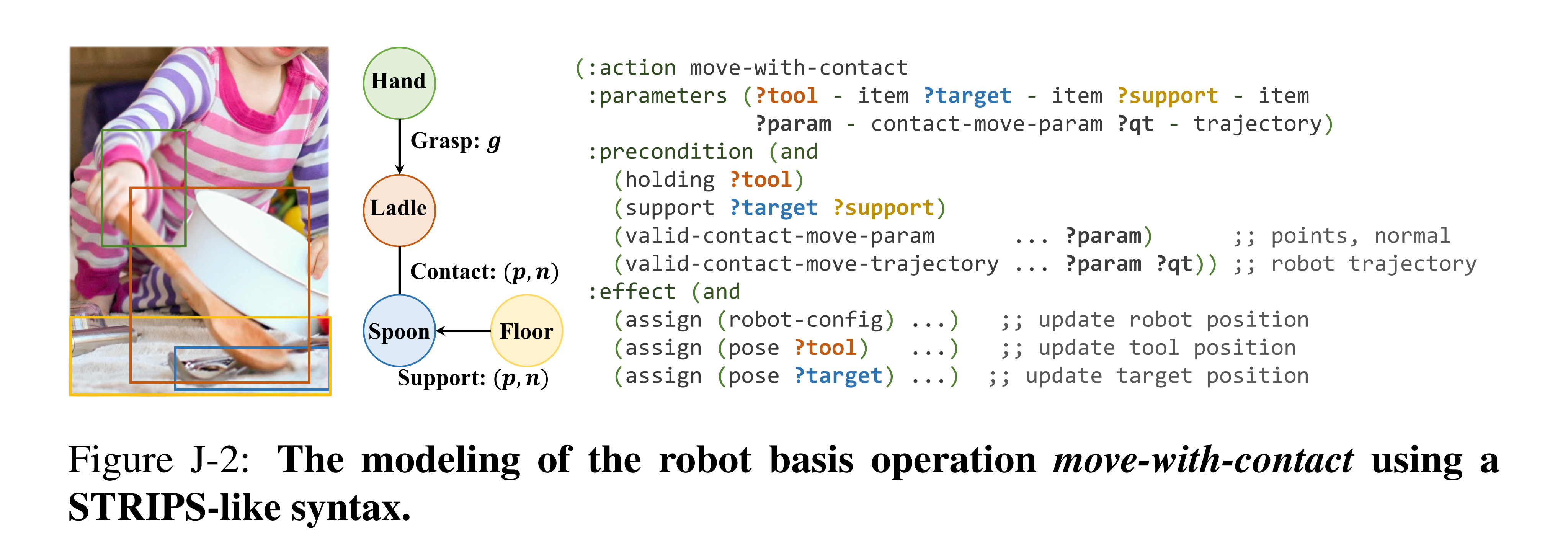
Figure J-2: The modeling of the robot basis operation move-with-contact using a STRIPS-like syntax.
Samplers for Generic Operations
Grasp sampling seeks opposing parallel surfaces, acceptable gripper width and inverse-kinematic reachability. Placement aligns sampled surfaces with a near-upward support normal; contact sampling excludes force into the support. BiRRT connects arm configurations, while pushing samples 5–25cm motion along the contact normal. The text says three variable types but lists four. Its printed grasp alignment equation uses an unnormalized point difference equal to one; retain it as source notation, not a dimensionally established general criterion.
Experiment Detail
The experiments use explicit object collections and feasible canonical configurations, then evaluate learned sampler efficiency and two physical mechanisms.
Mechanism Learning Setup
Six mechanism families use small sets of familiar meshes: edge pushing, hooking, levering, poking, stable placement and slope blocking. Every object is assigned a manually selected feasible canonical pose; both training and test instances perturb it by at most ±5cm and ±15°. Generalization here is within those designed neighborhoods, not arbitrary object arrangements.
Sampler Learning
The hook-use breakdown shows that generic search spends most samples on tool grasp and tool-target contact. Mechanism-specific scores sharply reduce those burdens. This explains the runtime benefit without implying that every motion-planning component becomes equally easy.
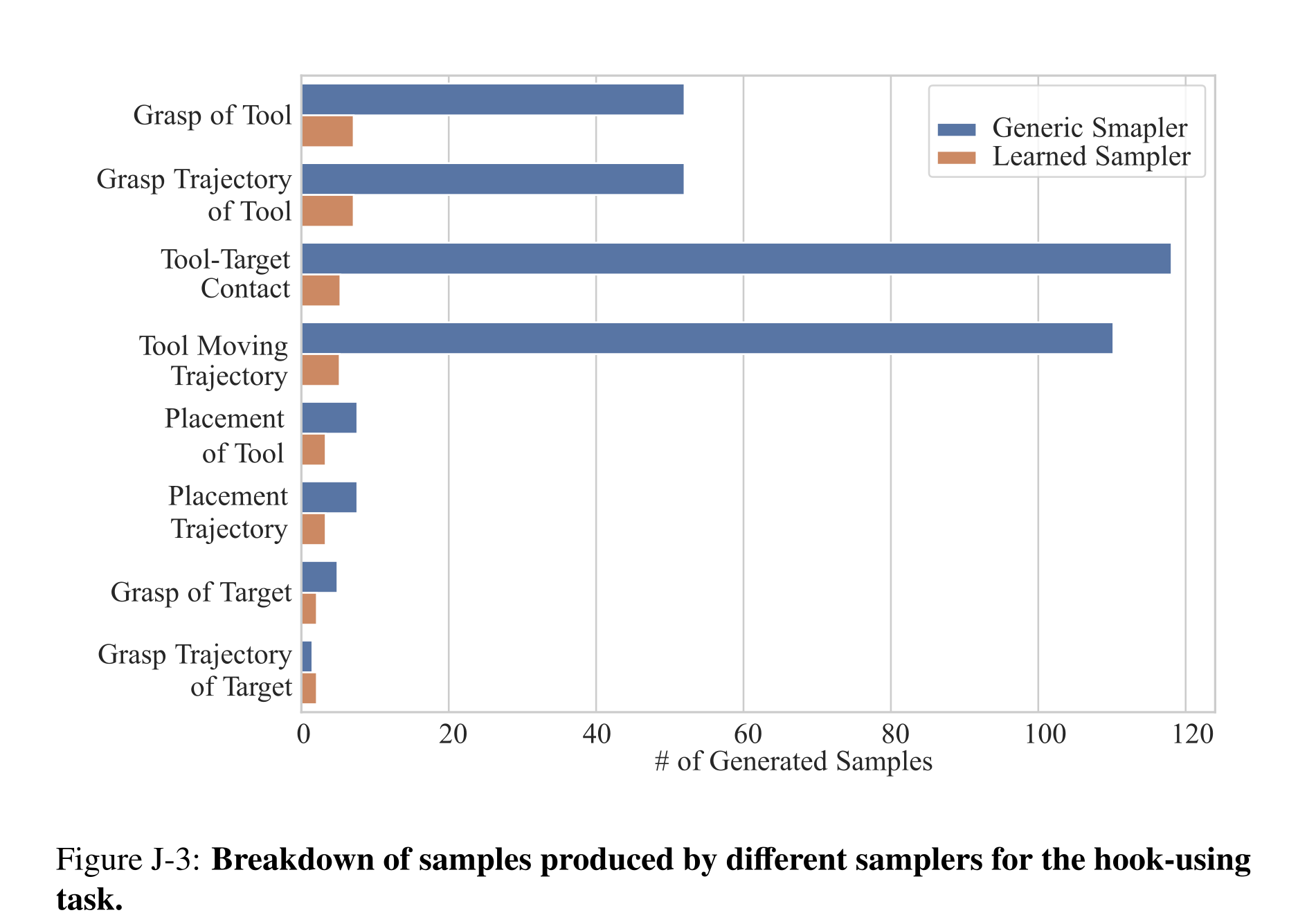
Figure J-3: Breakdown of samples produced by different samplers for the hook-using task.
Physical Robot Deployment
A calibrated D435/Franka pipeline segments partial point clouds, reconstructs objects by extrusion to the table, plans in PyBullet and executes with replanning after pushes/placements or detected grasp failure. Ten trials per task yield 80% edge-pushing and 70% hook-use success using the same object set at different initial poses.
Two plate failures push it off the table. Hook failures include unstable tip grasps and geometry invented by incomplete reconstruction; the system cannot recover from the latter case. Closed-loop observation helps invalid-grasp failures but does not eliminate perception/model mismatch.
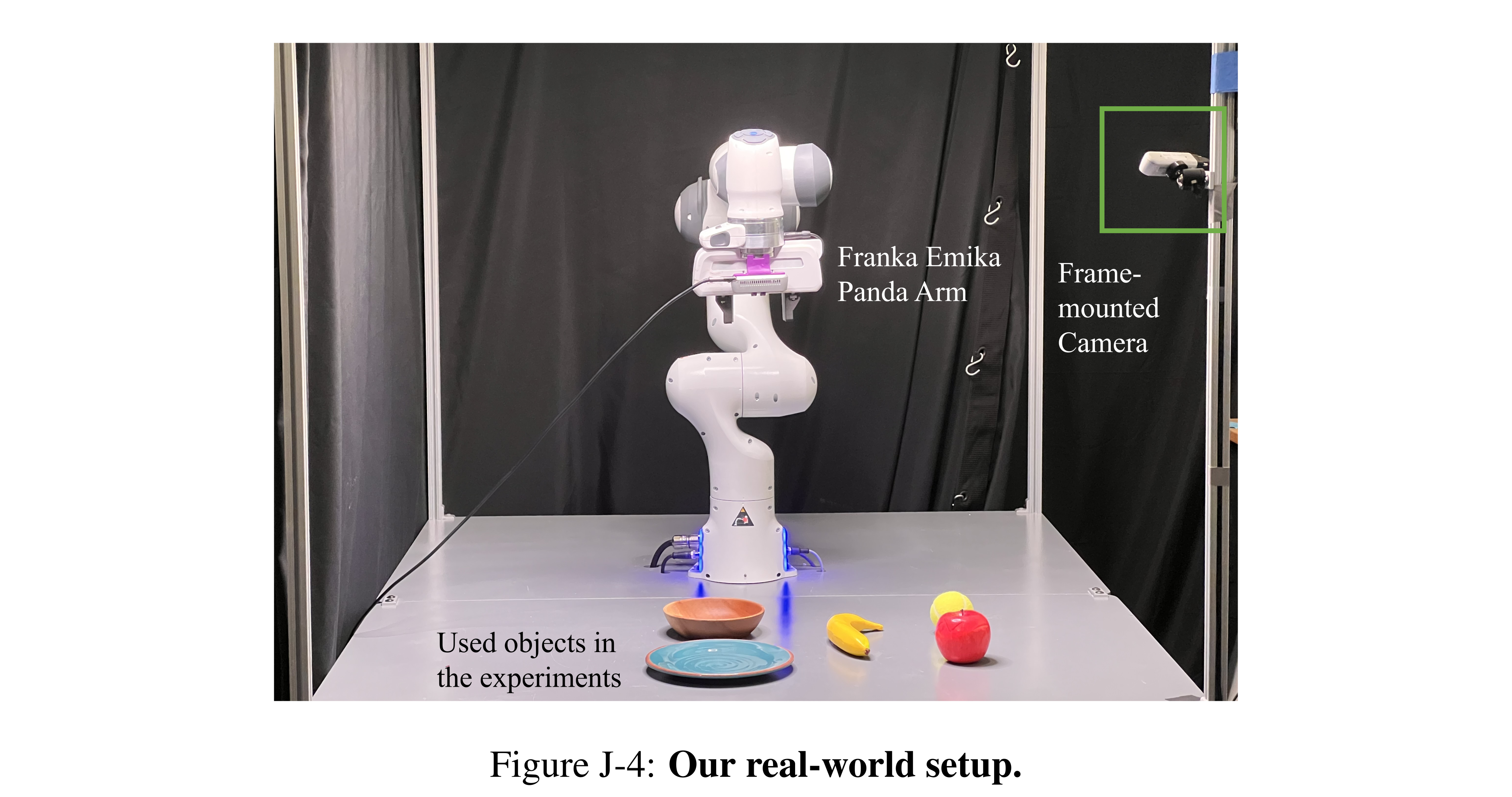
Figure J-4: Our real-world setup.

Table J.1: Success rate of our physical robot setup on two representative mechanisms.
Appendix for PDSketch
The appendix adds data-efficiency/on-policy results, a PDSketch language reference, heuristic compilation details and exact domain setups. It clarifies both the value and the cost of supplied structure.
Additional BabyAI Results
Additional BabyAI experiments measure executed-plan success, rather than only model-prediction accuracy. Separate on-policy experiments reveal that successful interactive learning depends strongly on built-in transition knowledge.
Data Efficiency and Variance Analysis
Across three runs, 100-demonstration success is 24% for behavior cloning, 23% for decision transformers, 4% for both PDS-Base and PDS-Abs, and 72% for PDS-Rob. Thus low-data model-based superiority is not uniform. With 1,000 demonstrations PDS-Abs reaches 98% and PDS-Rob 99%; at 10,000 PDS-Base reaches 80%. The strongest tiny-data result supplies robot dynamics, substantially reducing what must be learned.
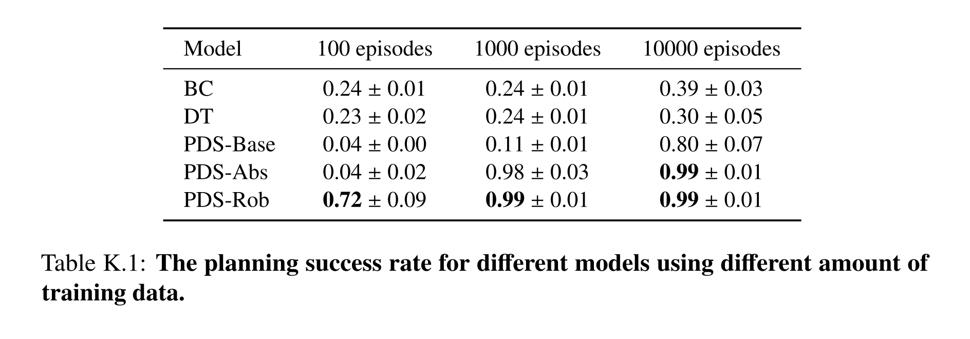
Table K.1: The planning success rate for different models using different amount of training data.
On-Policy Learning
The current model plans, executes in simulation, receives done labels and updates from the new trajectory without data reuse. PDS-Rob reaches 99% within 10,000 episodes, compared with a cited PPO requirement of 200,000. Direct on-policy PDS-Base/Abs stall around 6% because their early plans rarely succeed. Exploration and joint model/policy approaches are suggested remedies, not validated here. The main chapter points here for its lookahead loss, but this subsection discusses on-policy learning and does not provide that formula.
PDSketch Language
PDSketch defines a domain rather than a particular initial state or goal. Its Lisp-style syntax extends PDDL with typed vector features, derived predicates, unspecified neural functions, conditional effects and quantifiers. The listings are explanatory source examples, with occasional notation/syntax inconsistencies retained.
Predicate and Action Definition
Types distinguish objects from scalar/vector values; full hierarchical type inheritance is not supported. Input predicates read observations, derived predicates compose registered external functions, and shared neural blanks tie parameters across objects. Actions specify arguments, applicability and feature updates; varying the sketch ranges from detailed local dynamics to an unrestricted object-centric transition network.
Preconditions describe when a controller is applicable and should be supervised from its feasibility signal. Conditional effects describe how an executable action changes state and should be supervised from outcomes. The forward/pickup examples illustrate learned obstacles and selected objects, while PDS-Rob later supplies more of that knowledge. One early robot-facing example omits direction even though the complete implementation uses it; the example should not be read as a sufficient facing model by itself.
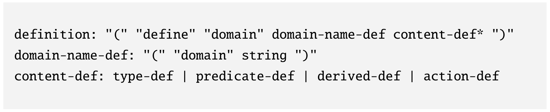
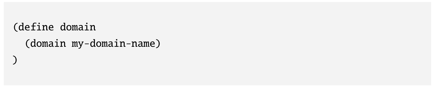
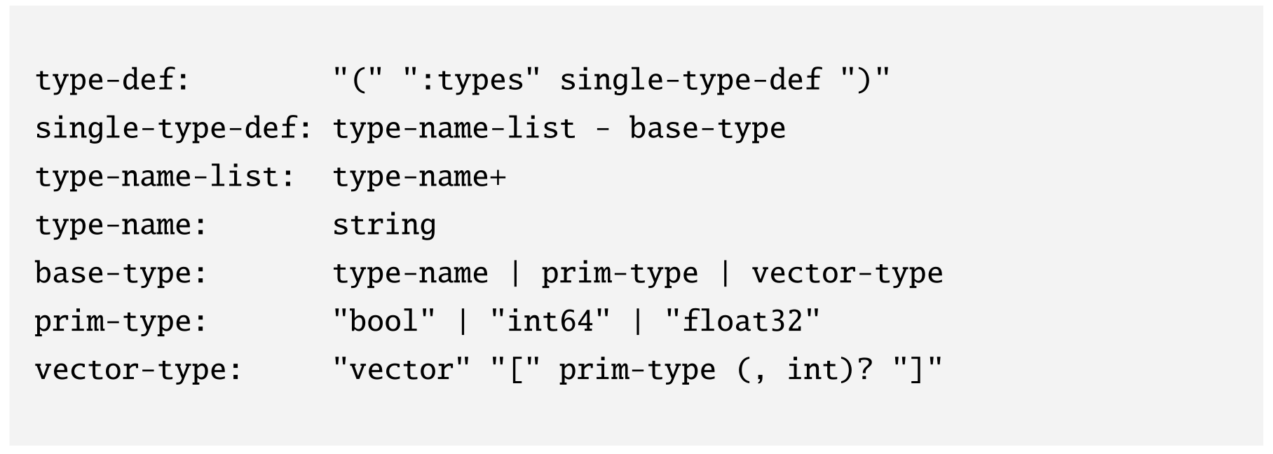
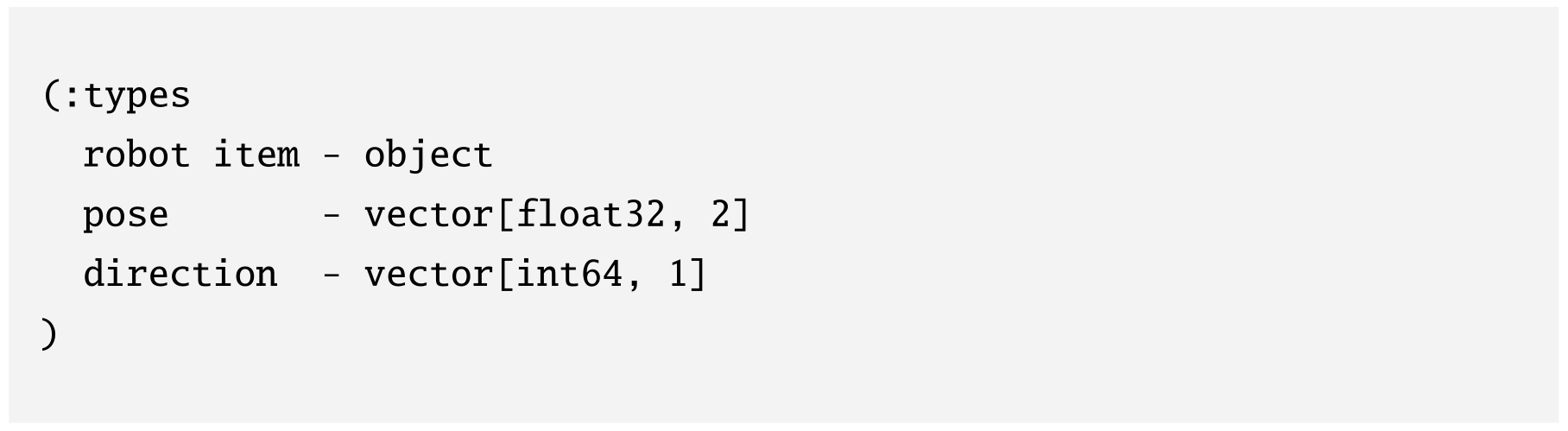
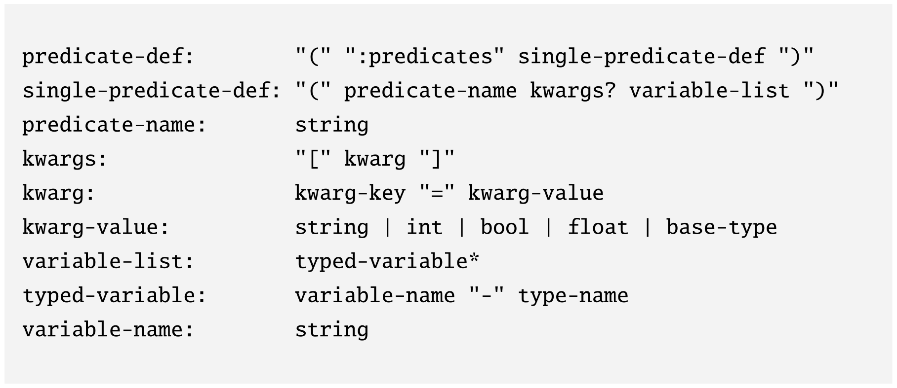
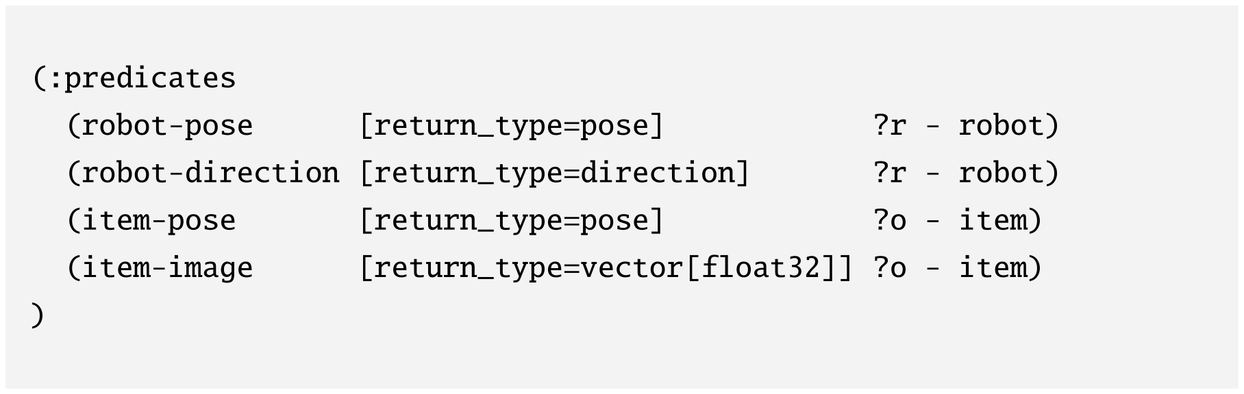

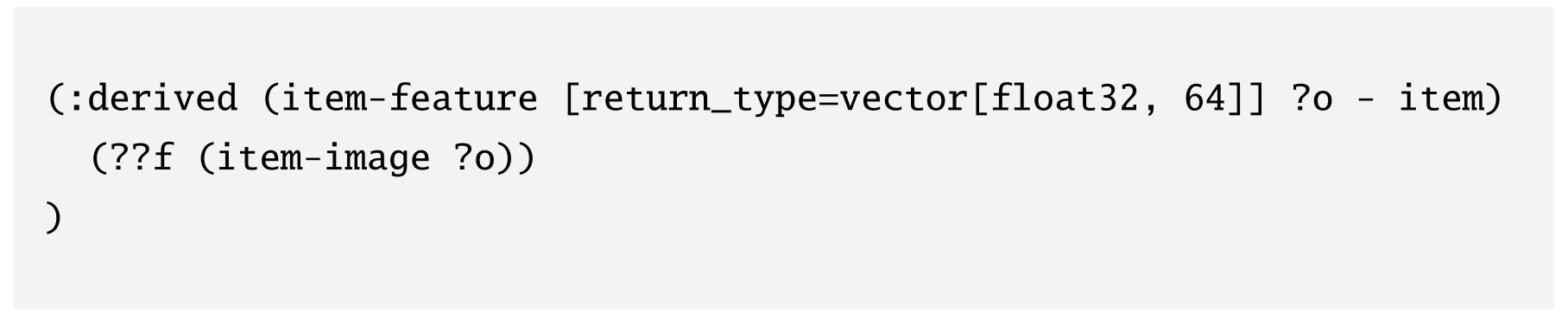

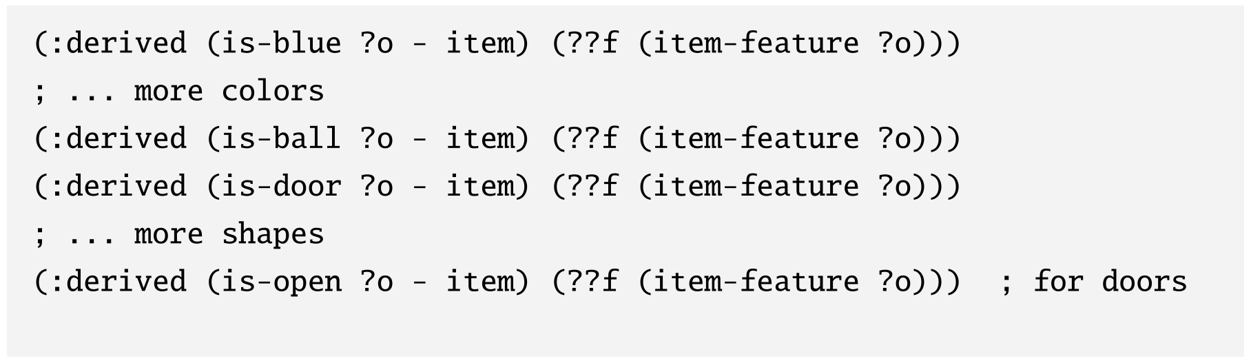
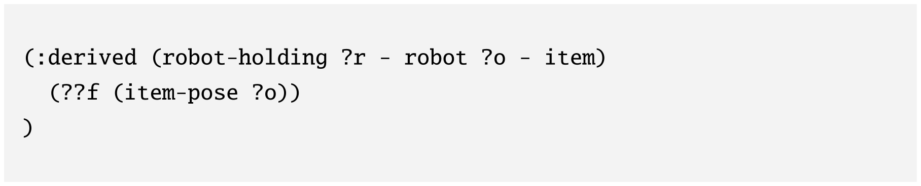
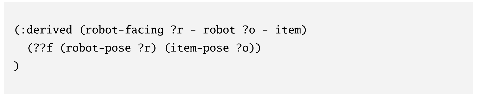
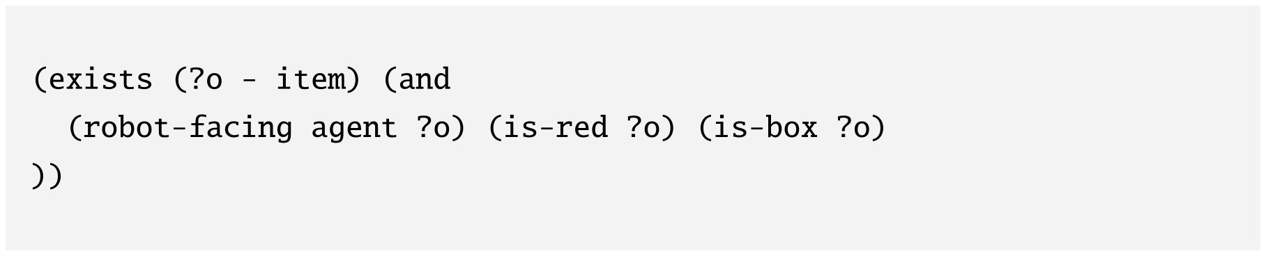
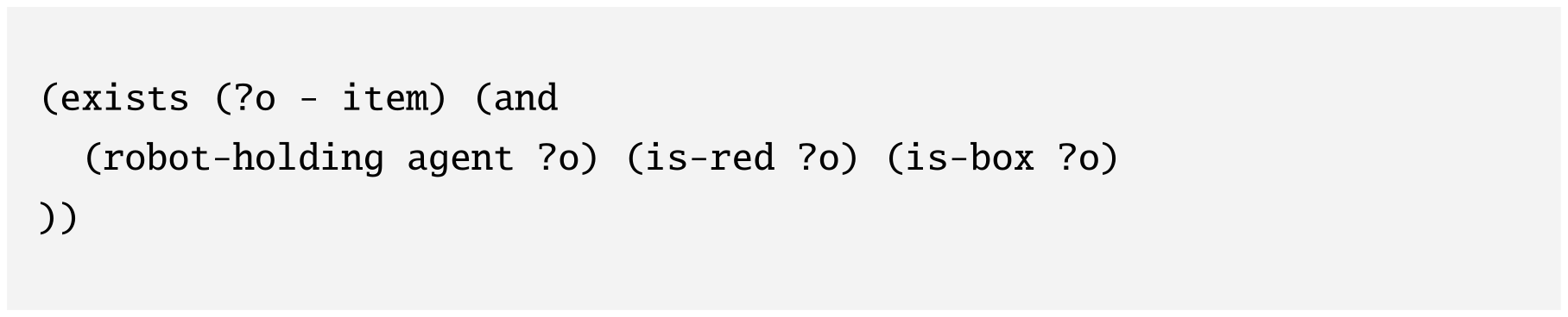
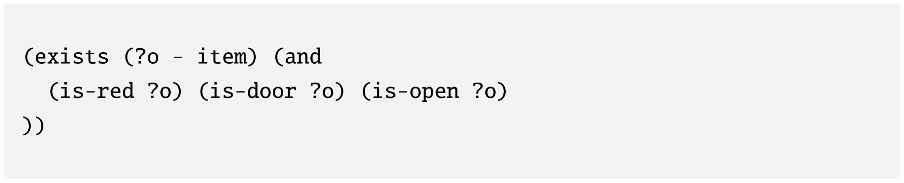
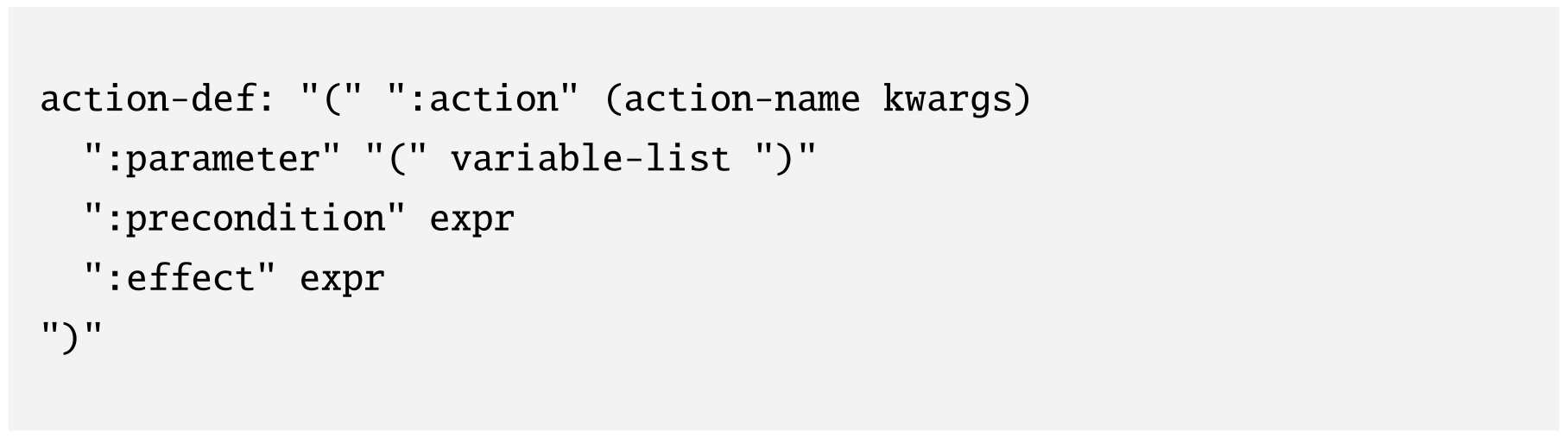
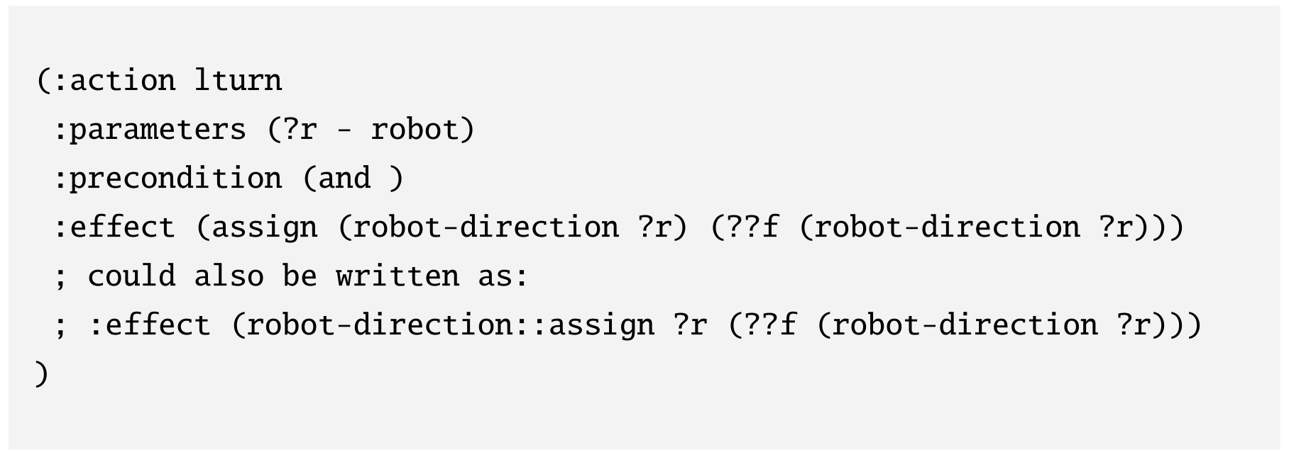
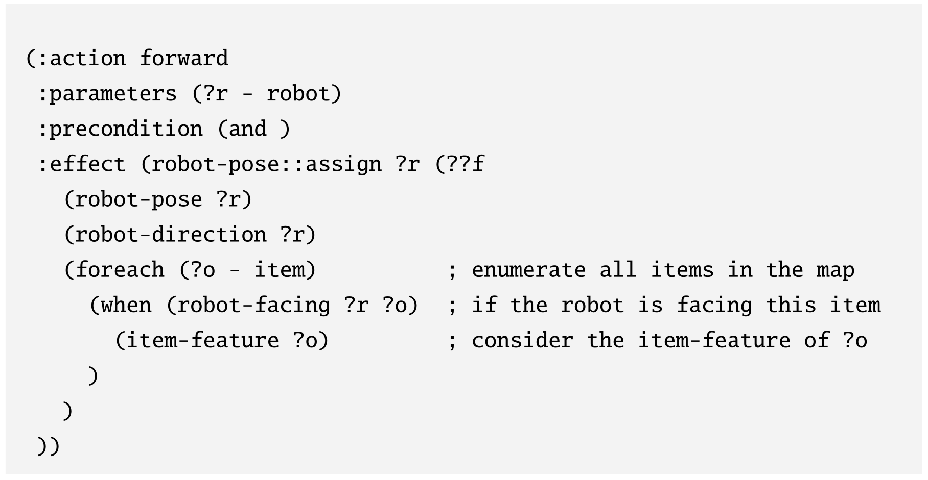

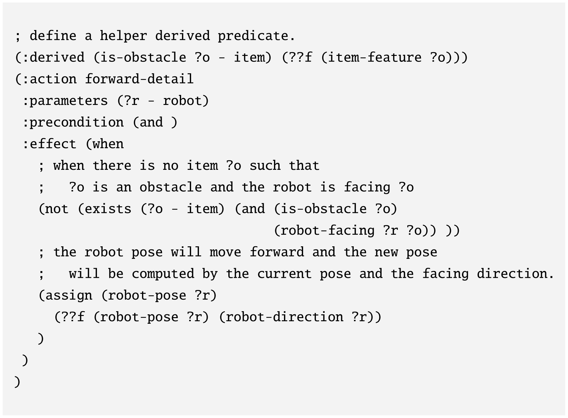
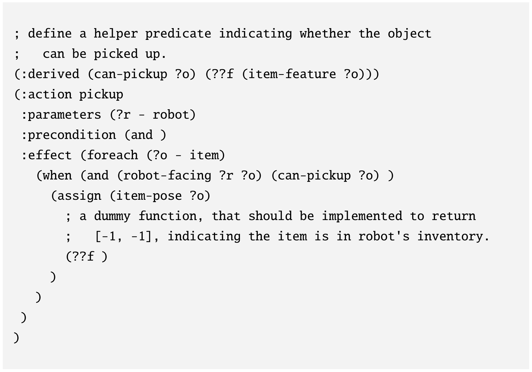
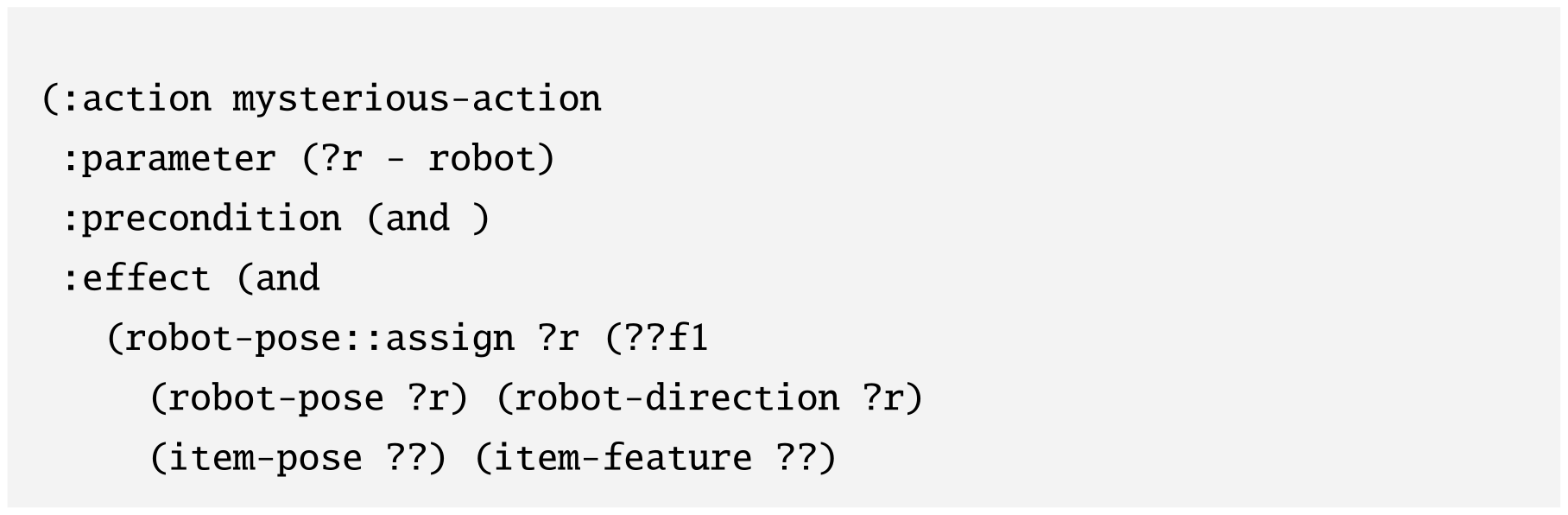
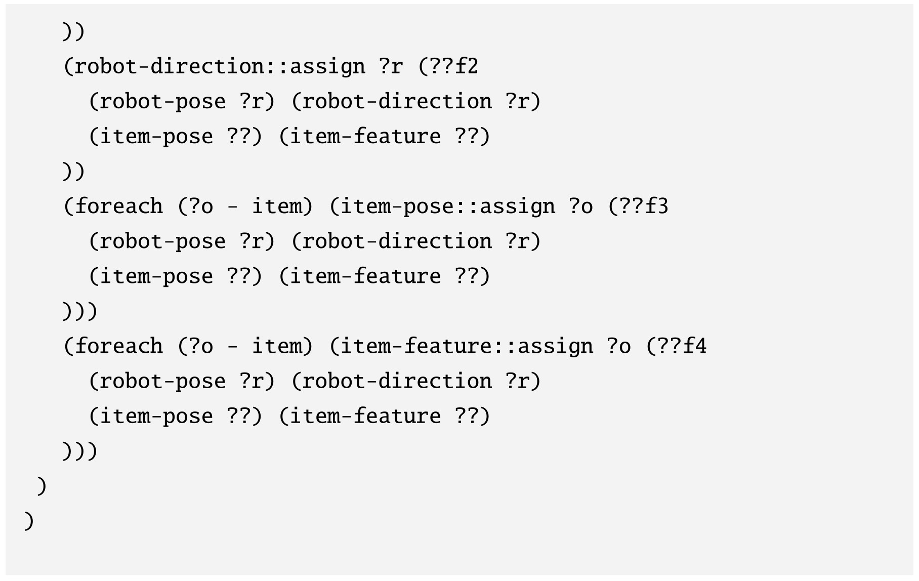
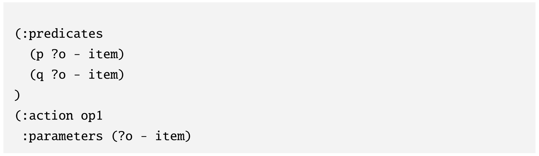
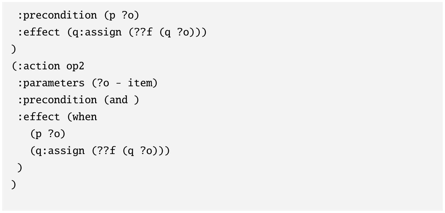
Expressions
Boolean connectives and finite quantifiers use min/max soft logic; assignment changes features, foreach iterates over objects, and when selects relevant inputs or gates effects depending on context. Shorthands expose conditional assignment/selection, and ?? names externally implemented functions. The source says a negated Boolean effect assigns true; that is inconsistent with the usual delete-effect semantics and is a source typo, not a rule to implement silently.
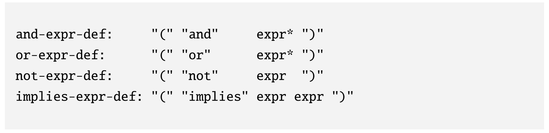
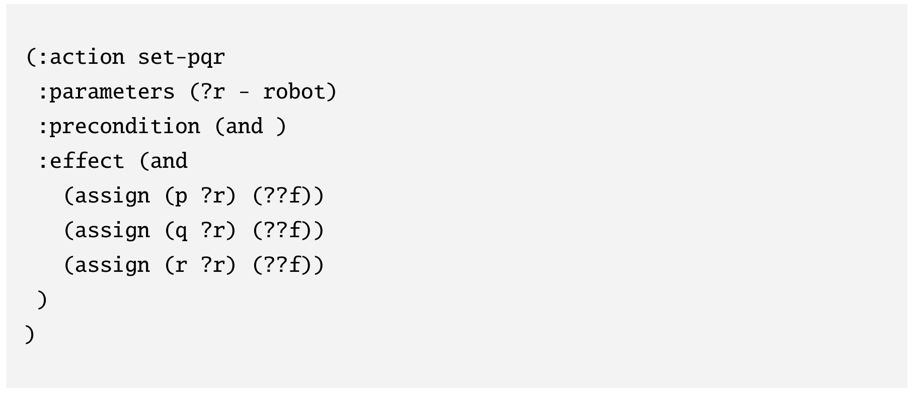




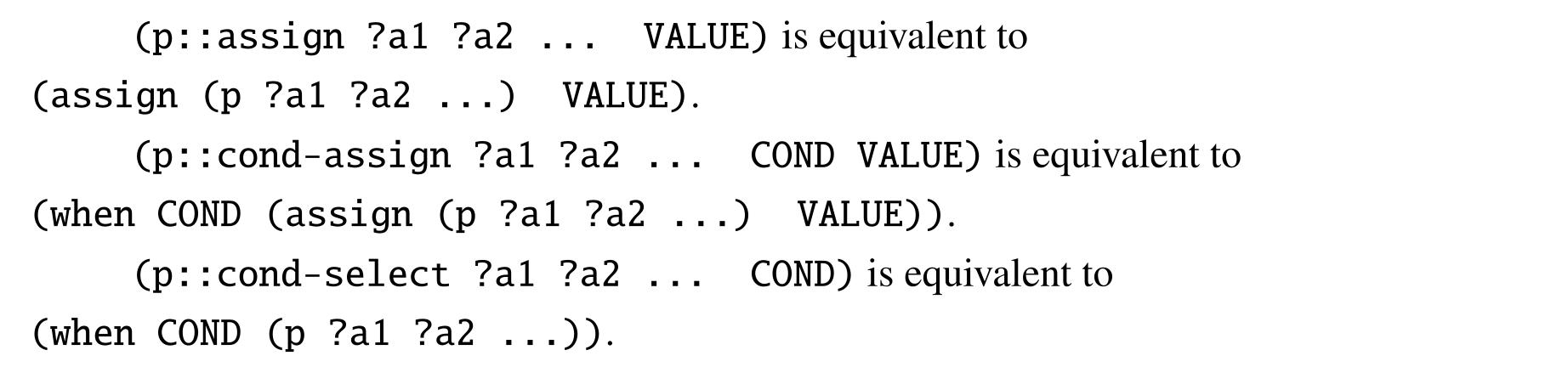

Domain-Independent Heuristic
Optimistic compilation treats a changed non-Boolean feature as able to satisfy any test, exploiting locality but ignoring its value. And-Or compilation quantizes latent values, initializes codes with k-means, fine-tunes for one epoch and learns first-order decision rules with FOIL. It preserves more structure at greater compilation cost. Both guide search while leaving actual learned-model simulation unchanged.
Factorization prevents one giant categorical state space: separate x, y, color and shape codes require 24 component values in the example versus 1,176 combinations. The heuristic therefore benefits from the human-specified decomposition. The relaxed estimate is useful guidance, not a general admissibility/optimality claim.
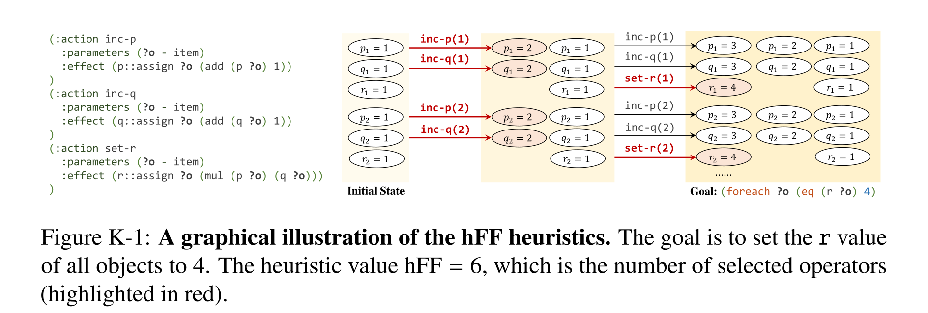
Figure K-1: A graphical illustration of the hFF heuristics. The goal is to set the r value of all objects to 4. The heuristic value hFF = 6, which is the number of selected operators (highlighted in red).
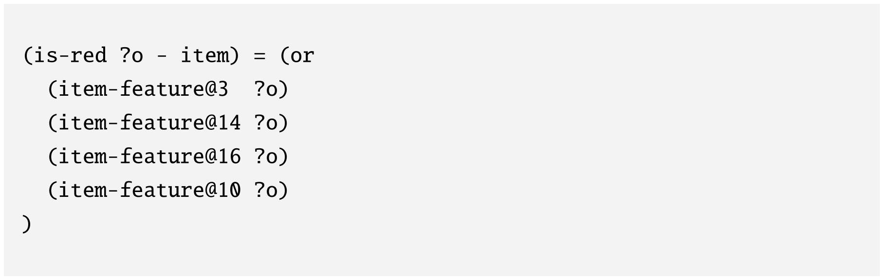
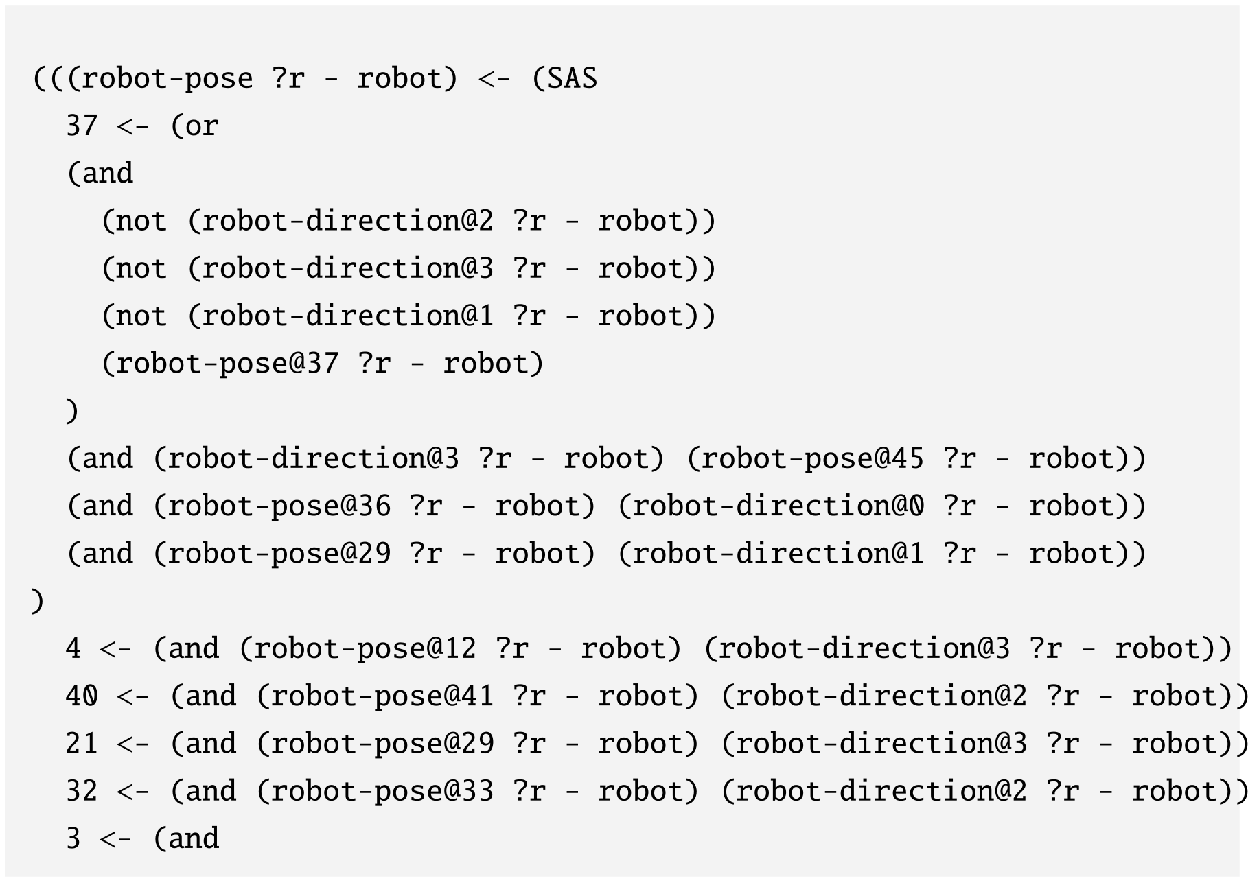
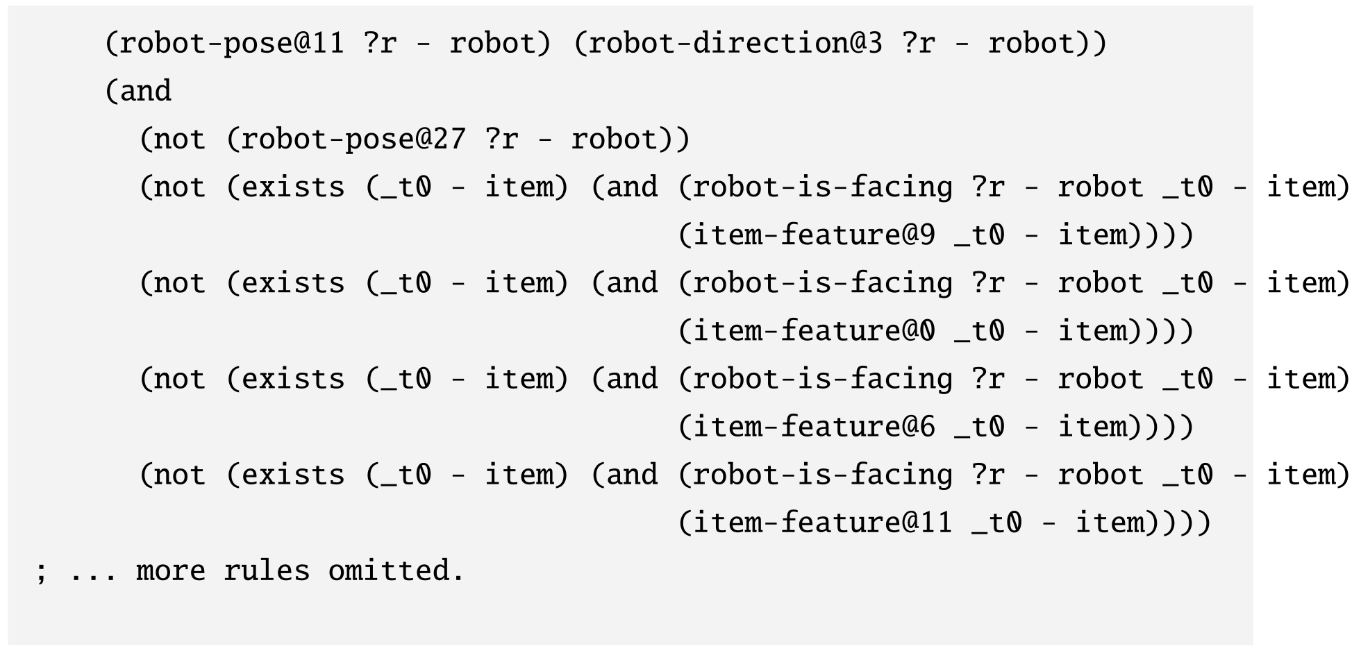
Experimental Setup
The concrete setups specify input encodings, demonstrations, baselines and human model knowledge, which are necessary for interpreting comparisons.
BabyAI
BabyAI demonstrations use A* successes and failures generated by approaching a wrong object then taking five random steps. Baselines receive object-state embeddings, numeric positions, direction embeddings and encoded goals, processed with two-layer GNNs. This is more structured input than unconstrained raw images.
PDS-Base mixes object pose/appearance; PDS-Abs separates them and introduces facing-based dependence. PDS-Rob additionally supplies the facing-position computation and is-obstacle information as input, not only a vague architectural prior. Its data-efficiency advantage therefore includes externally provided transition/obstacle knowledge.
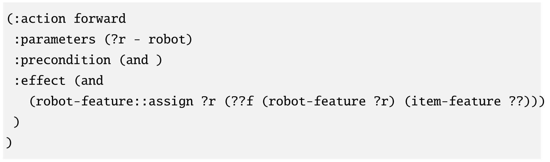
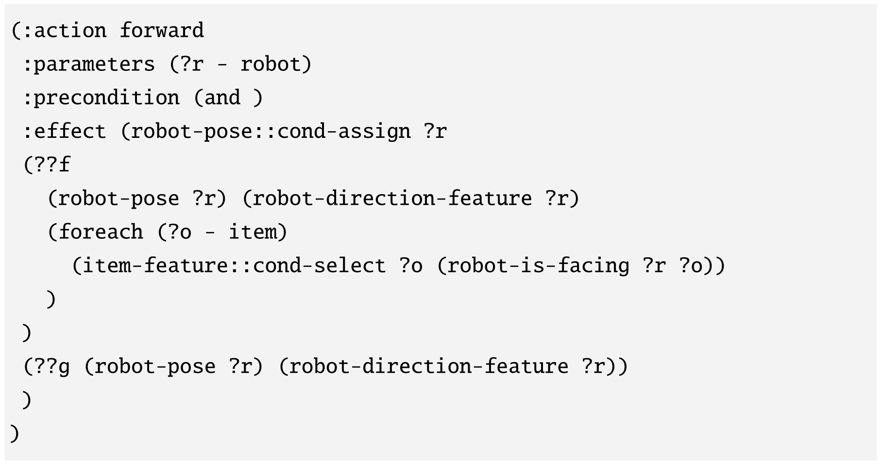

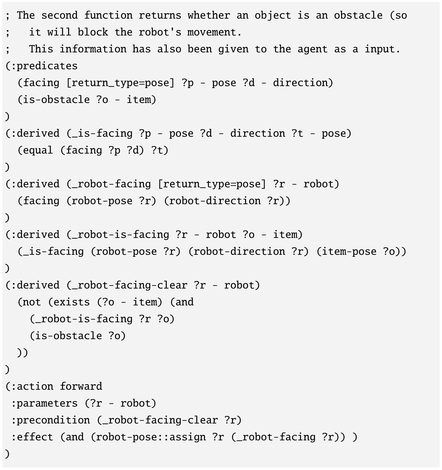
Painting Factory
Painting represents each detected object/container by a 32×32 crop and normalized xyz location; a CNN produces 128-dimensional visual features. Scripted two-block demonstrations supervise container placement and direct placement. GNN baselines score discrete object/container choices and predict a location for direct moves.
Continuous planning samples poses satisfying learned on/left/right relations, then instantiates actions in a PDDLStream-style planner. The printed sigmoid uses squared distance minus a threshold, whereas the prose describes closeness; without the sign constraint on its learned temperature, that formula should not be silently interpreted as an ordinary decreasing distance classifier.
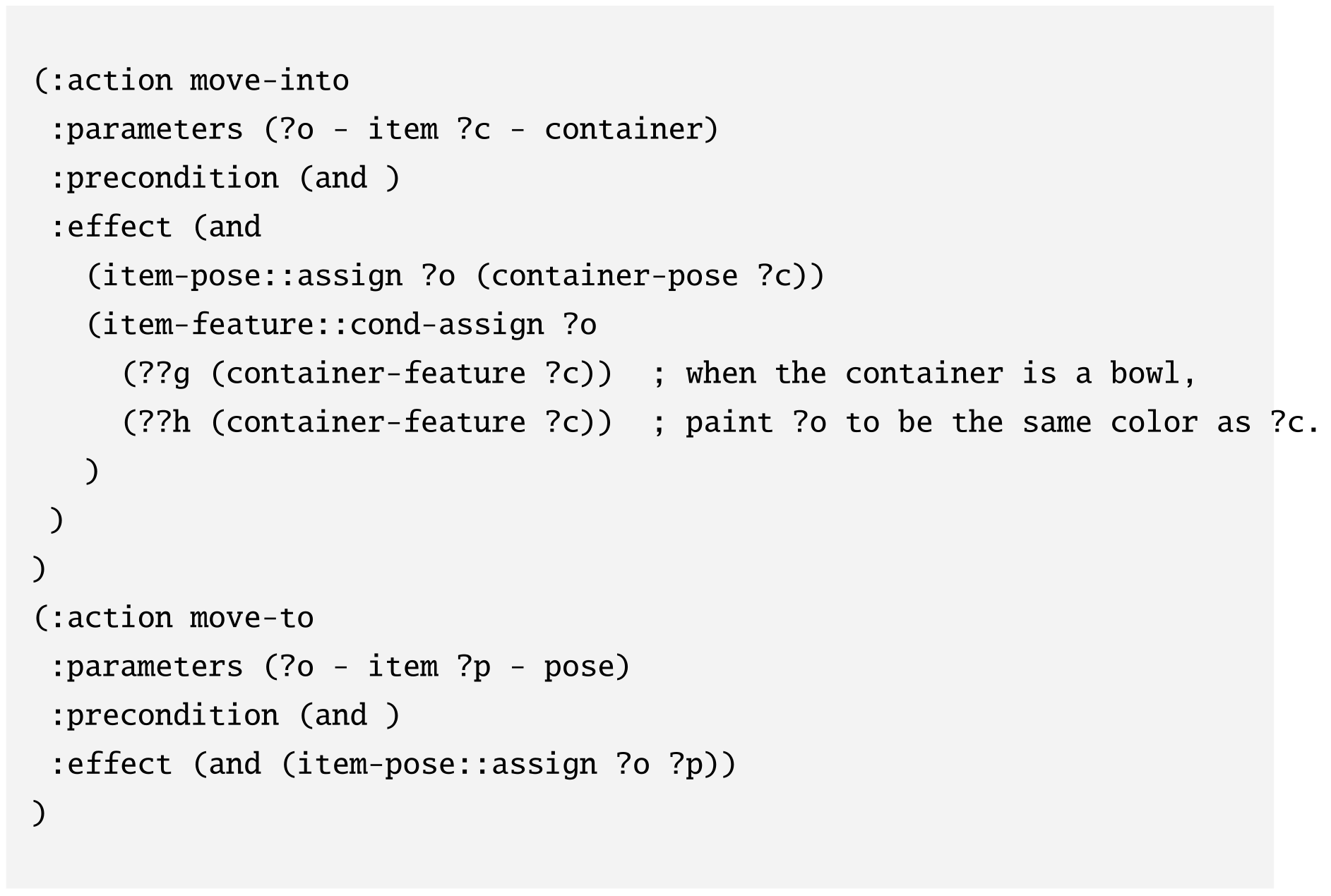
Equation

Appendix for Behavior from Language and Demonstration
The BLADE appendix supplies behavior-generation prompts/listings, segmentation and labeling algorithms, classifier/policy details, adapted baselines, all task definitions and qualitative traces. It reveals additional supervision and practical restrictions behind the main results.
BLADE Details
Behavior models, classifiers, policies and replanning form separate components. Automatically propagated state labels reduce manual labeling, but depend on supplied language/context, consistent contact segmentation and the validity of the generated symbolic model.
Behavior Description Generation with LLMs
Listings L.1–L.6 preserve generated CALVIN behaviors and the prompts defining contact primitives, environment/predicate vocabulary, worked examples and task input. Environment descriptions are explicitly provided; automatic image tagging is proposed as an alternative, not the reported default. The generated examples contain naming/arity inconsistencies such as lifted versus is-lifted, so they are source examples rather than a certified executable library.
Predicate Generation with LLMs
An additional experiment asks the LLM to propose predicates, ground their arguments and remove redundancies. It reports close matches for 28 of 30 expert predicates, with push-left/right confused through next-to. Generated real-world domains produce correct plans on the nine tested task cases, but this is not a complete re-evaluation of learned visual grounding and physical execution. Main quantitative experiments still use the supplied predicate vocabulary.
Temporal Segmentation
Segmentation assumes fully open grippers for free motion and fully closed grippers for pushing; demonstrators are instructed accordingly. Simulator contacts supply object arguments, while real-world arguments come from language annotations or an LLM. LLM-generated bodies correct extra leading/trailing primitives before retraining. More general grasps/contact interactions can violate these heuristics, and tested visual alternatives had inconsistent segmentation.
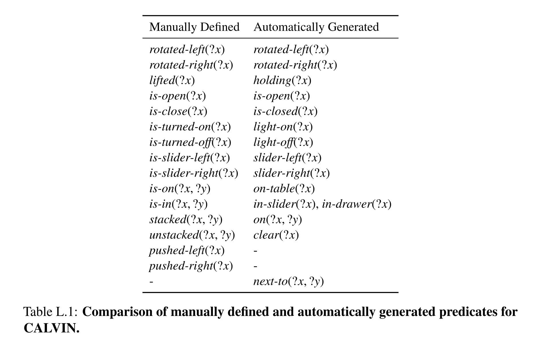
Table L.1: Comparison of manually defined and automatically generated predicates for CALVIN.
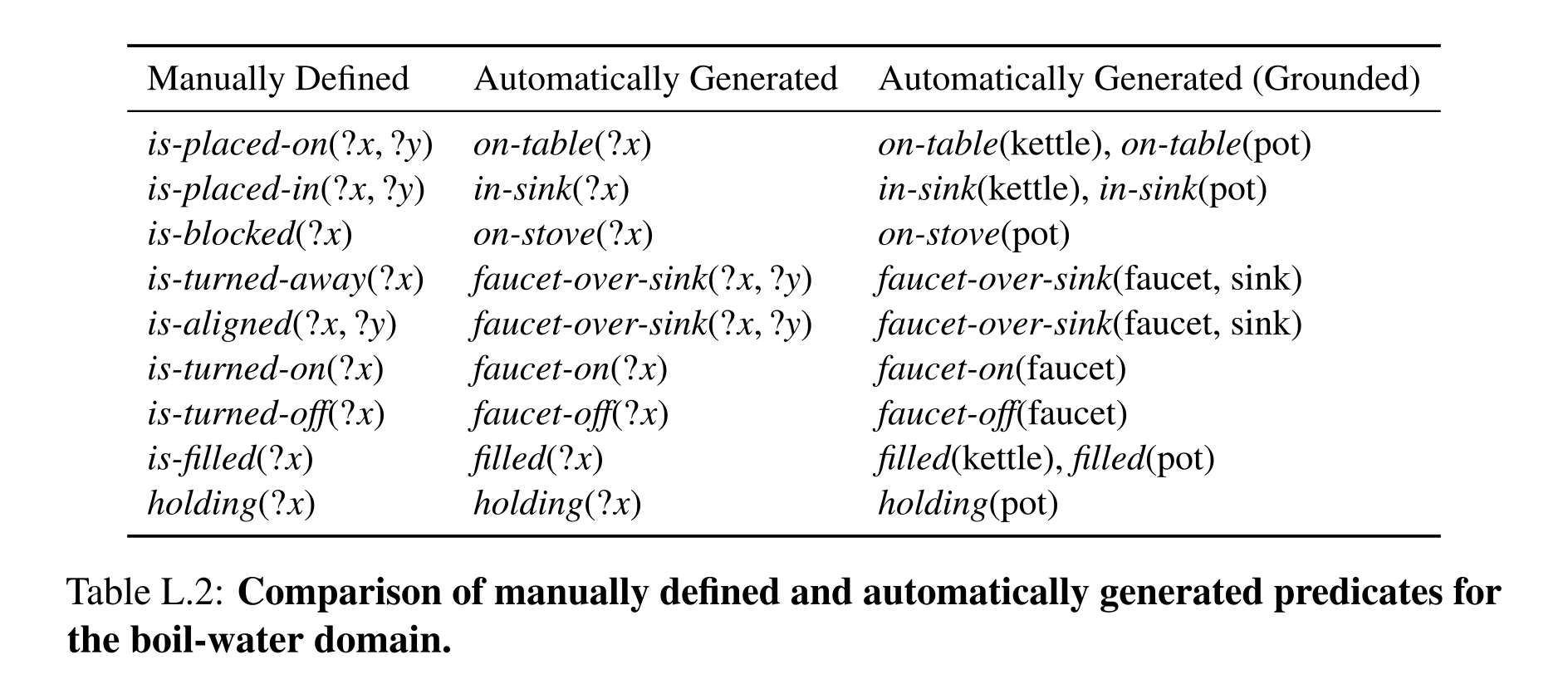
Table L.2: Comparison of manually defined and automatically generated predicates for the boil-water domain.
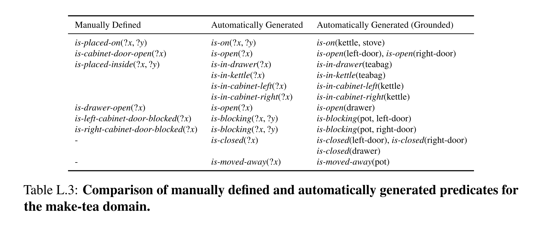
Table L.3: Comparison of manually defined and automatically generated predicates for the make-tea domain.
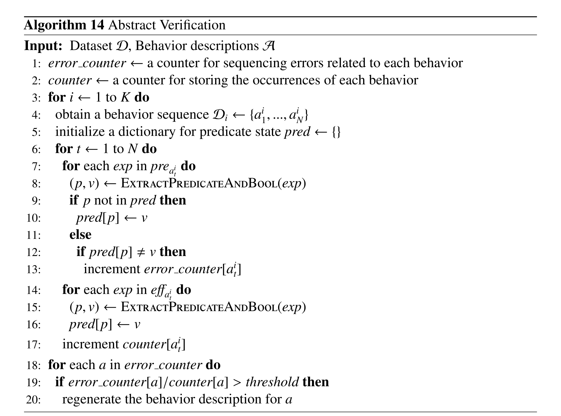
Abstract Verification
Algorithm 14 propagates known predicate values through behavior sequences, counts contradictions between preconditions and accumulated effects, and regenerates operators above an error threshold. Previously unknown preconditions are accepted and entered into the state. Thus the check detects contradictions on the demonstrations, not independent truth of every newly asserted precondition.
Automatic Predicate Annotation
Algorithm 15 produces positive/negative predicate examples from preconditions, effects and persistence between behaviors. Effects are negated before their action and asserted afterward; unchanged labels propagate. This is useful pseudo-supervision but assumes actions actually establish their listed effects and do not silently change unlisted predicates. Effects already true before execution can violate the assumed negative label.
Classifier Implementation
Simulation uses frozen CLIP ViT-B/32 patch tokens, robot-arm masking, argument embeddings and predicate-specific MLP heads. The real-world classifier instead uses Grounding-DINO object boxes to crop 3D regions, then a Point Cloud Transformer trained from scratch on combined object point clouds with identity channels. This detail is more specific than the main chapter’s image-crop description.
Replacing trained classifiers with GPT-4o gives 0% Boil Water task success in the reported test, despite better recognition of articulated states than spatial relations. Visual examples from the annotation procedure improve VLM accuracy by about 5% on 220 held-out examples in a preliminary study; no corresponding successful end-to-end result is reported.
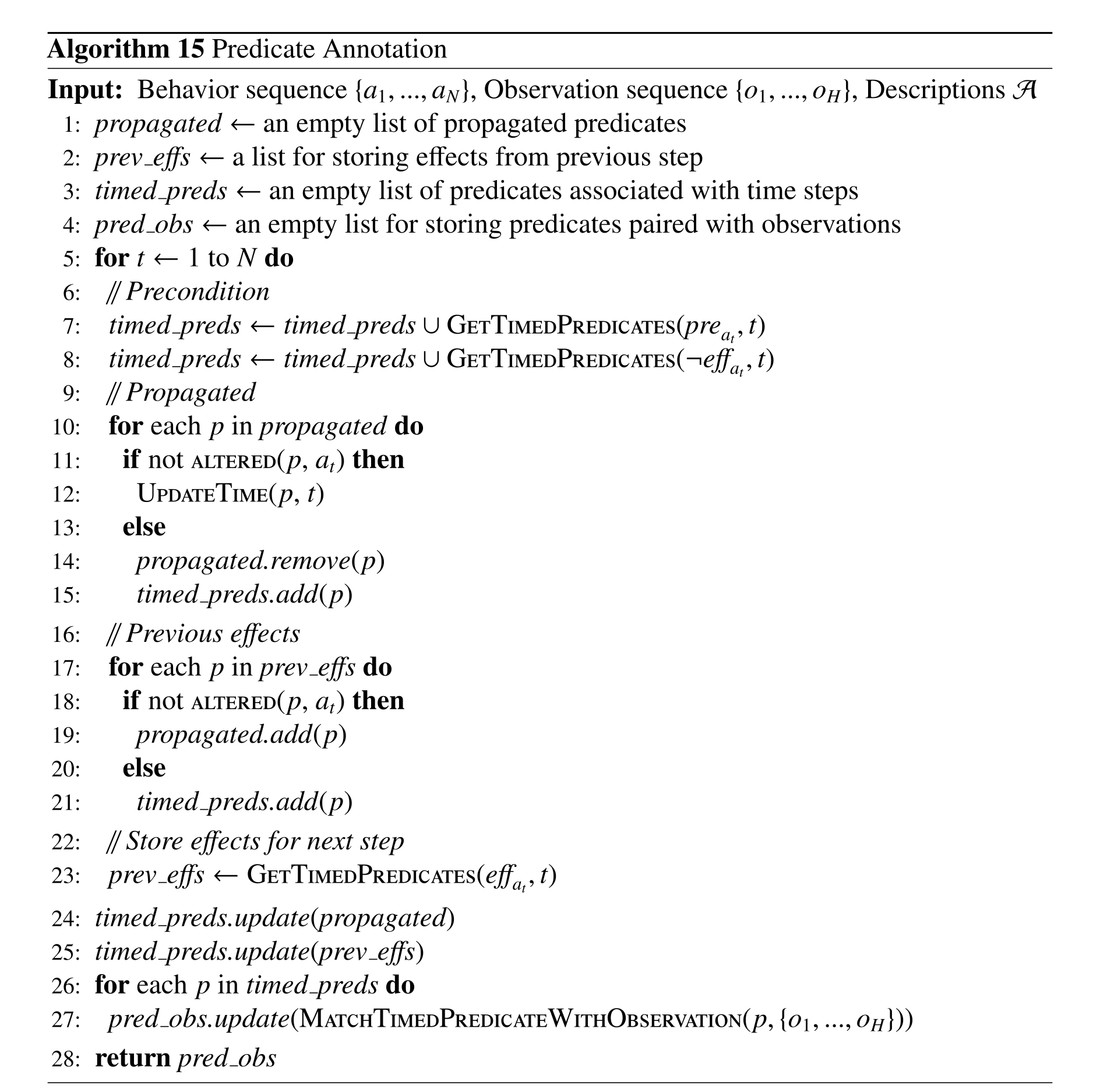
Policy Implementation
Diffusion policies randomize preceding history for the initial action, bias sampling toward diverse start poses and append zero-action tails for termination. Simulation uses relevant-object point clouds with ground-truth segmentation masks and a PCT/time-series encoder. Real hardware uses five separate ResNet-34 image encoders and predicts world-frame gripper poses. These design choices and simulator masks are part of the comparison setting.
Planner Implementation
Geometric blocking constraints are checked immediately before execution, after planning semantic preconditions, because the model does not predict exact future object poses. The planner recursively clears blockers when needed; this assumes sufficient free space and does not solve tightly coupled rearrangement generally. Hidden-object search uses optimistic deterministic effects and observation/replanning; explicit belief distributions and observation planning are future extensions.
Simulation Experiment Details
The simulator retains CALVIN’s original skills, annotations, action space and environment but introduces six new evaluation tasks for composition and recovery. These are new task specifications on CALVIN, not its ordinary single-skill evaluation alone.
Task Design
Three abstract-goal tasks turn off both lights or place all three blocks in an initially open/closed drawer. Two partially observable tasks retrieve a block from a closed drawer or behind the slider. The geometric task moves a slider obstructed by a block, judged within 5cm of its target end. Variants change block color or slider direction; task samplers and explicit goal checks define success.
Baseline Implementation
HULC is the hierarchical baseline; HULC++ is omitted to focus on planning. SayCan is adapted to detected objects and a demonstration-trained image feasibility model instead of RL Q-functions. Robot-VILA uses GPT-4-turbo-2024-04-09 with accumulated image/text history. Text2Motion-Shooting uses a multistep feasibility model and either ground-truth or BLADE-classified symbolic states. These are documented adaptations, so results should not be generalized to every original baseline implementation.
Qualitative Examples
Figures L-4–L-6 show representative failures of baseline loops, misplaced blocks, hidden-object handling and blocked-slider actions, alongside successful BLADE sequences. These illustrative traces explain possible failure mechanisms; the aggregate table is the quantitative evidence.
Real World Experiment Details
Each physical domain contributes 85 SpaceMouse demonstrations recording end-effector pose, gripper width and five calibrated RGB-D views. Four cameras are fixed and one wrist-mounted. The same recorded demonstrations train state classifiers and policies.
Task Design
Boil Water tests an already-in-sink kettle, a human moving it after faucet alignment, and a blocked stove; its goal includes a filled kettle on the stove with the faucet off. Make Tea tests open-door starts, a drawer reclosed by a person, blocked cabinet doors and a hidden kettle; the goal is kettle placement plus teabag insertion. The prose says six tasks but lists seven generalization cases; together with two original-sequence conditions these match the nine plotted real-world conditions. Filling/placement are the evaluated goals, not actual thermal boiling or brewed-tea quality.
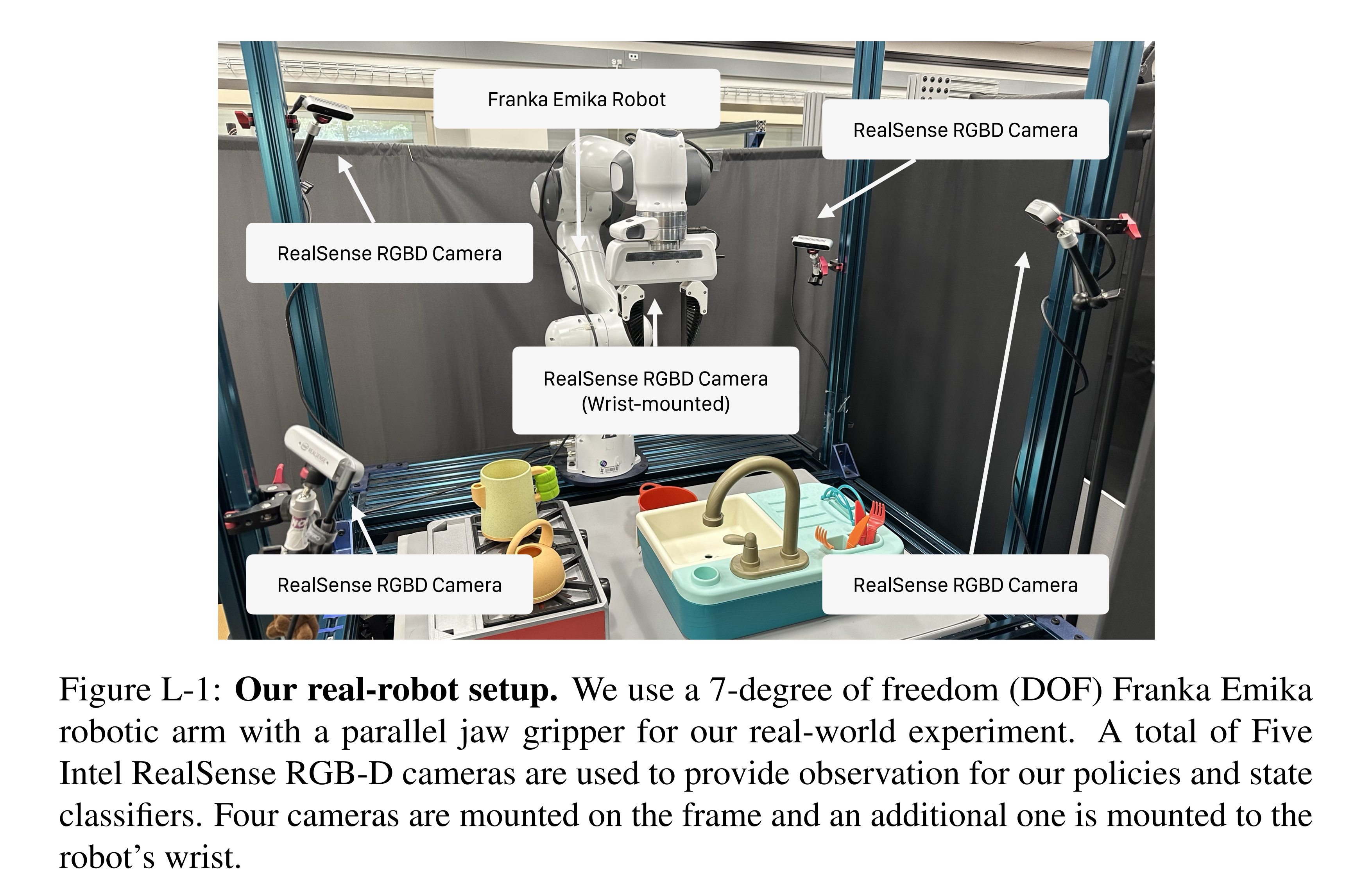
Figure L-1: Our real-robot setup. We use a 7-degree of freedom (DOF) Franka Emika robotic arm with a parallel jaw gripper for our real-world experiment. A total of Five Intel RealSense RGB-D cameras are used to provide observation for our policies and state classifiers. Four cameras are mounted on the frame and an additional one is mounted to the robot’s wrist.
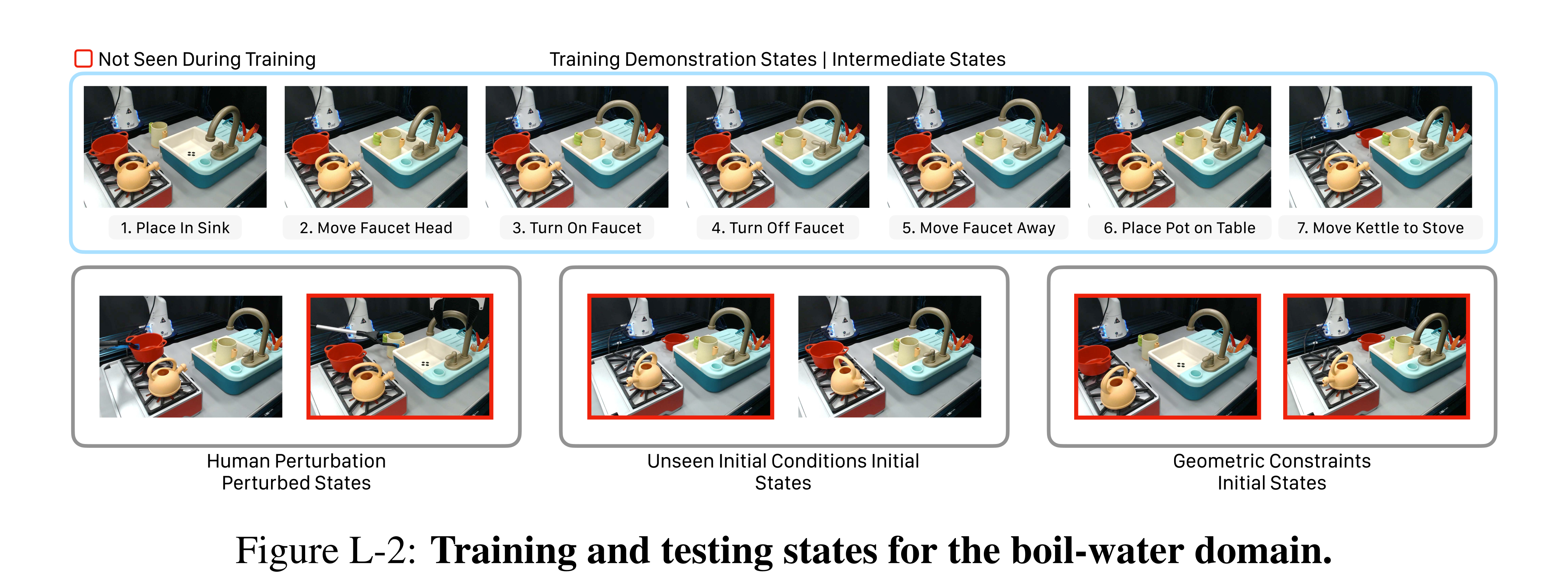
Figure L-2: Training and testing states for the boil-water domain.
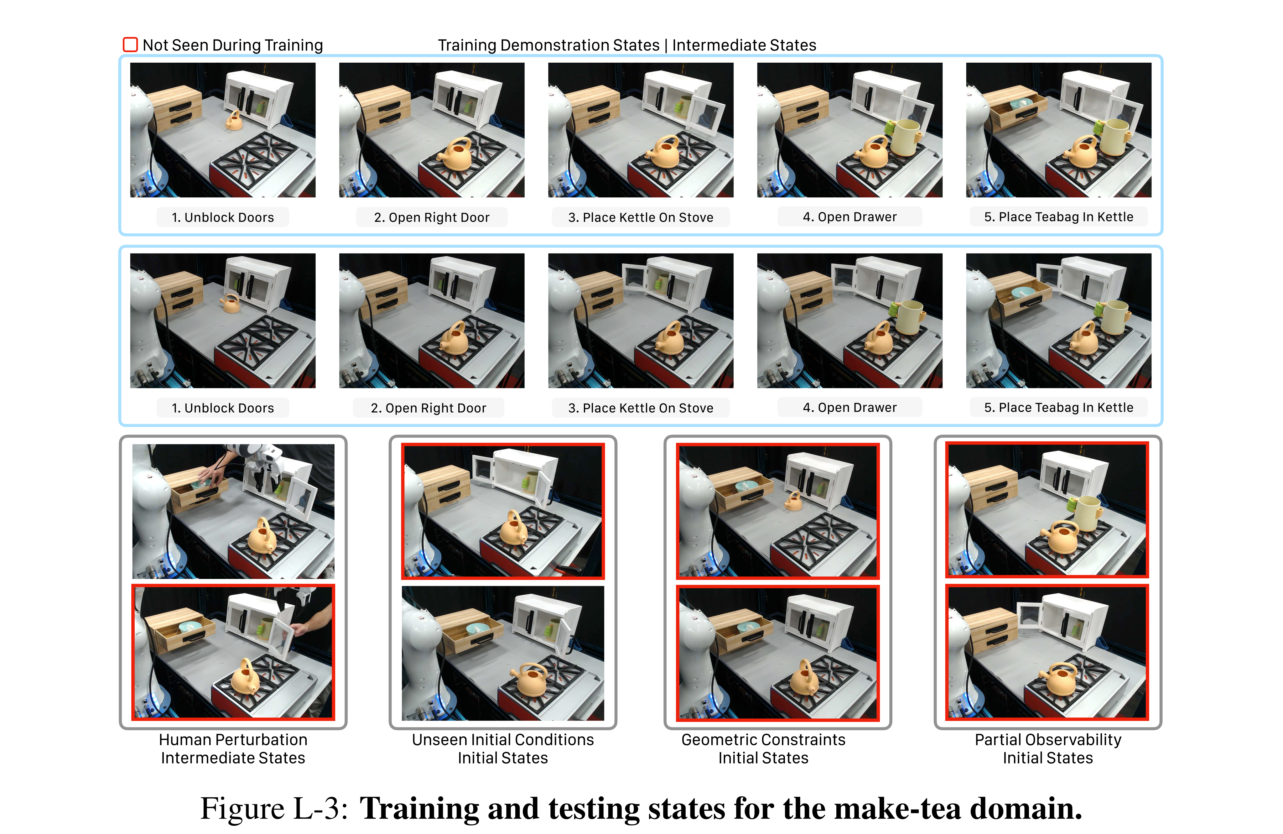
Figure L-3: Training and testing states for the make-tea domain.
Qualitative Examples of Novel States
Figures L-2/L-3 contrast training sequences with novel initial and perturbed states. The authors state that over half these test states are absent from demonstrations. This supports the need for recomposition but does not prove that all imitation-based alternatives must fail.
Prompts for Baselines
The complete listings preserve SayCan candidate-ranking prompts, Robot-VILA initial and follow-up visual planning prompts, and Text2Motion symbolic-state examples. They specify action vocabularies, environment context and output formats. Some source examples mix predicate/action spellings and SayCan’s printed template includes a current symbolic-state field despite the simpler high-level description; retain the source and interpret comparisons through the detailed implementation, rather than silently standardizing their prompts.
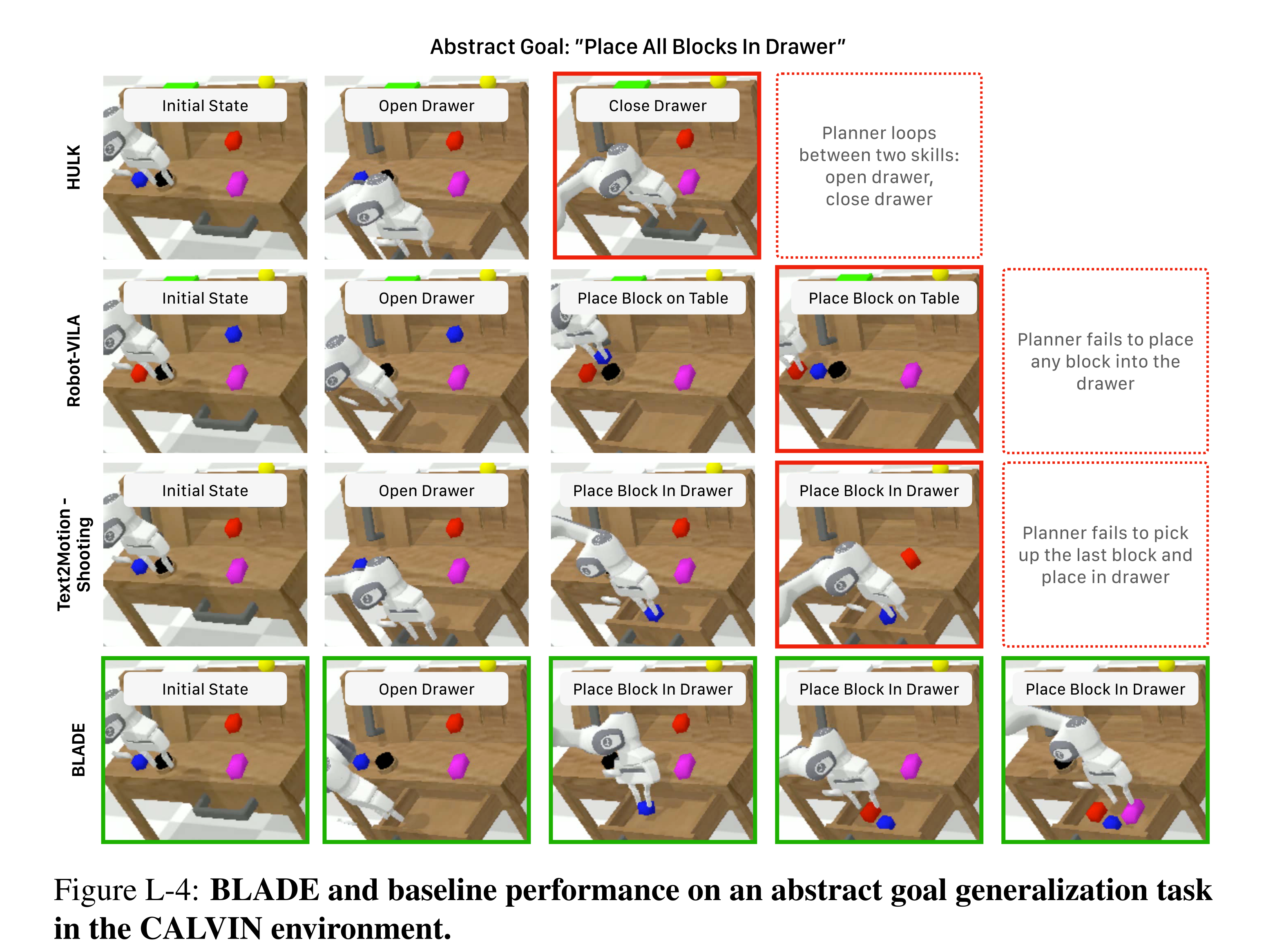
Figure L-4: BLADE and baseline performance on an abstract goal generalization task in the CALVIN environment.
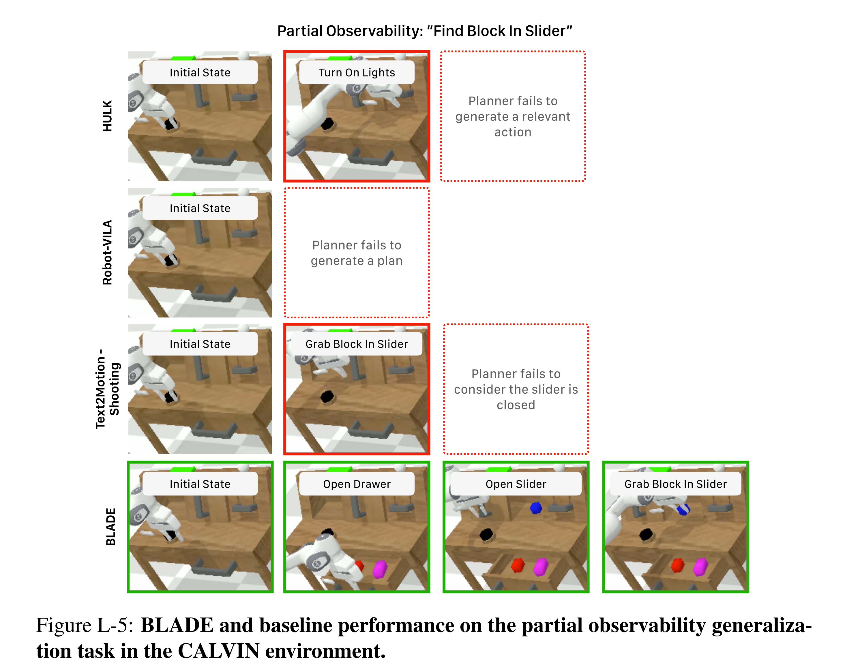
Figure L-5: BLADE and baseline performance on the partial observability generaliza- tion task in the CALVIN environment.
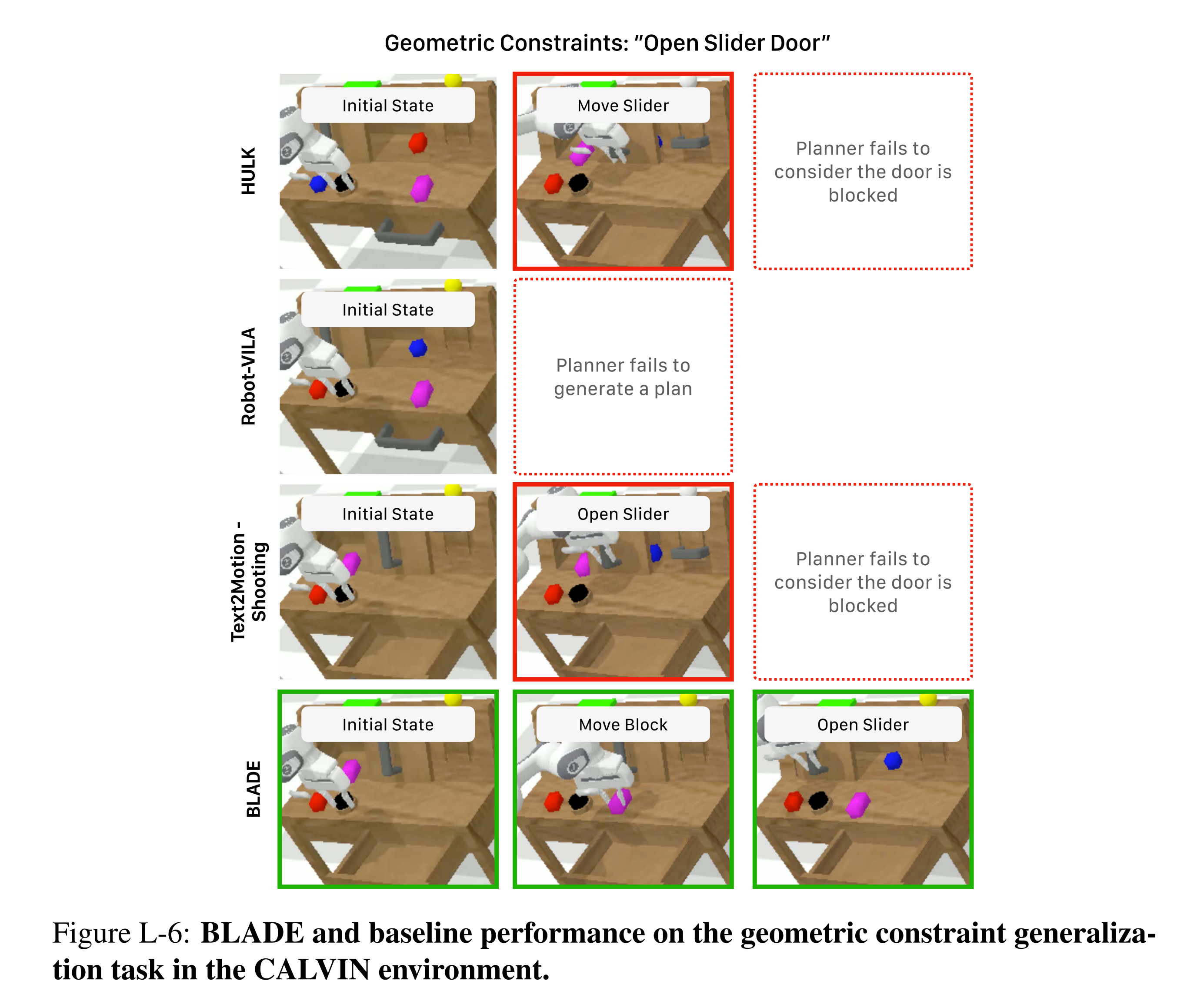
Figure L-6: BLADE and baseline performance on the geometric constraint generaliza- tion task in the CALVIN environment.
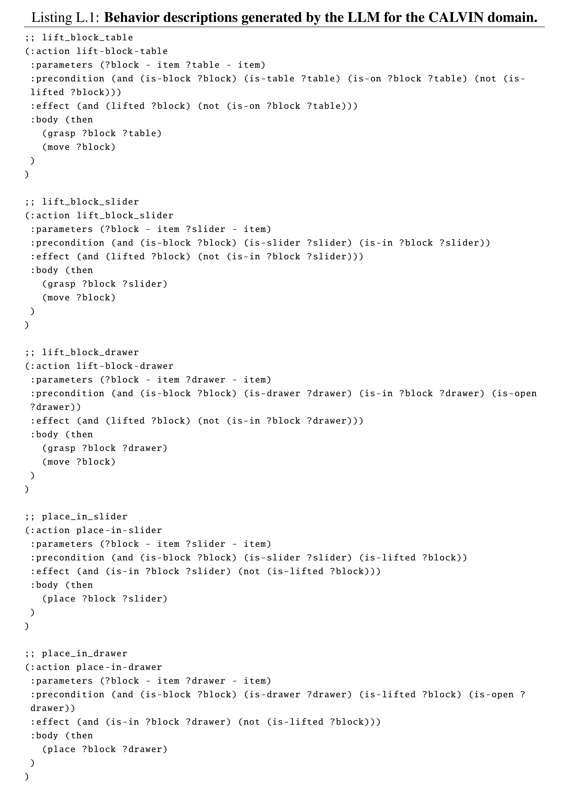
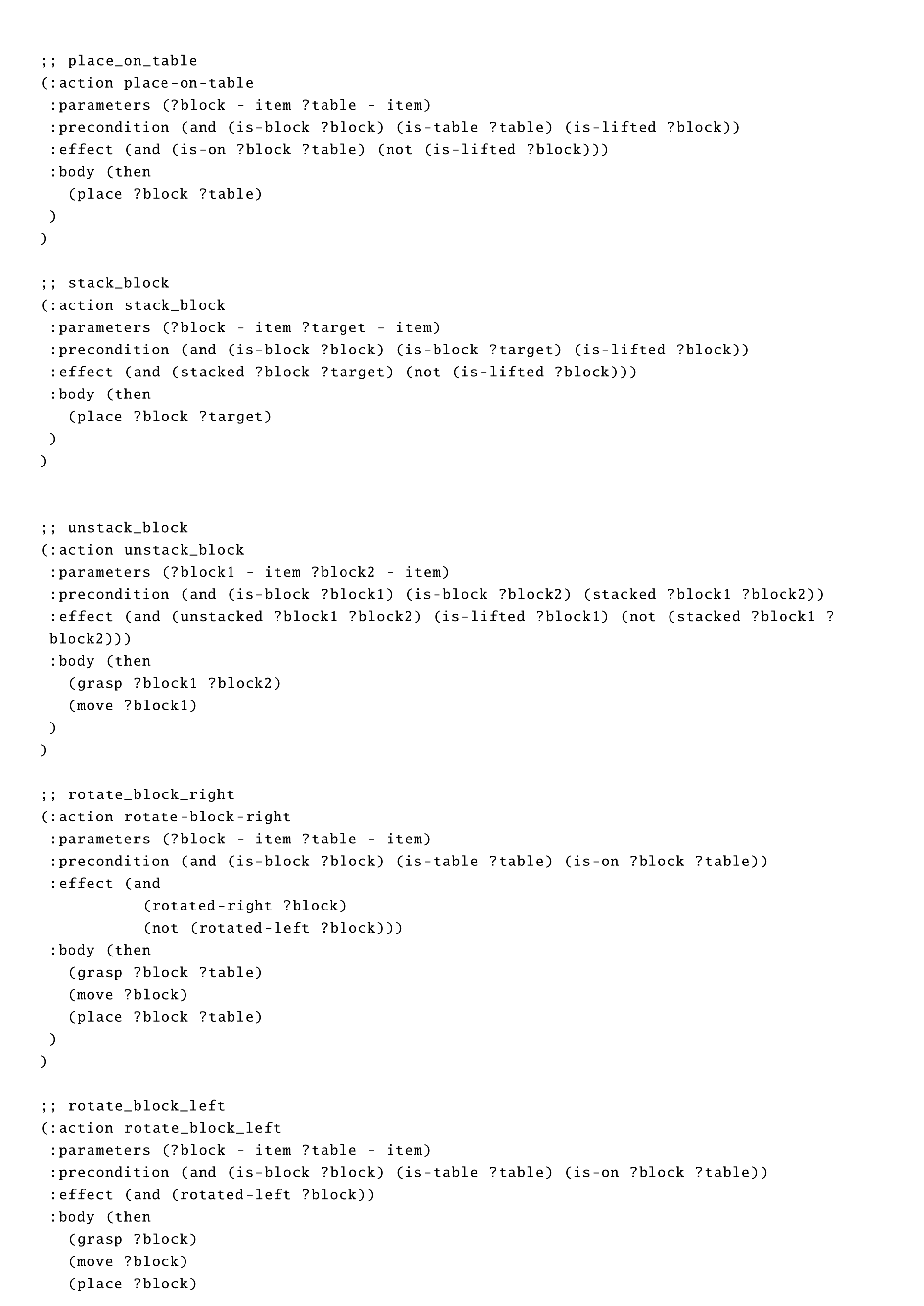
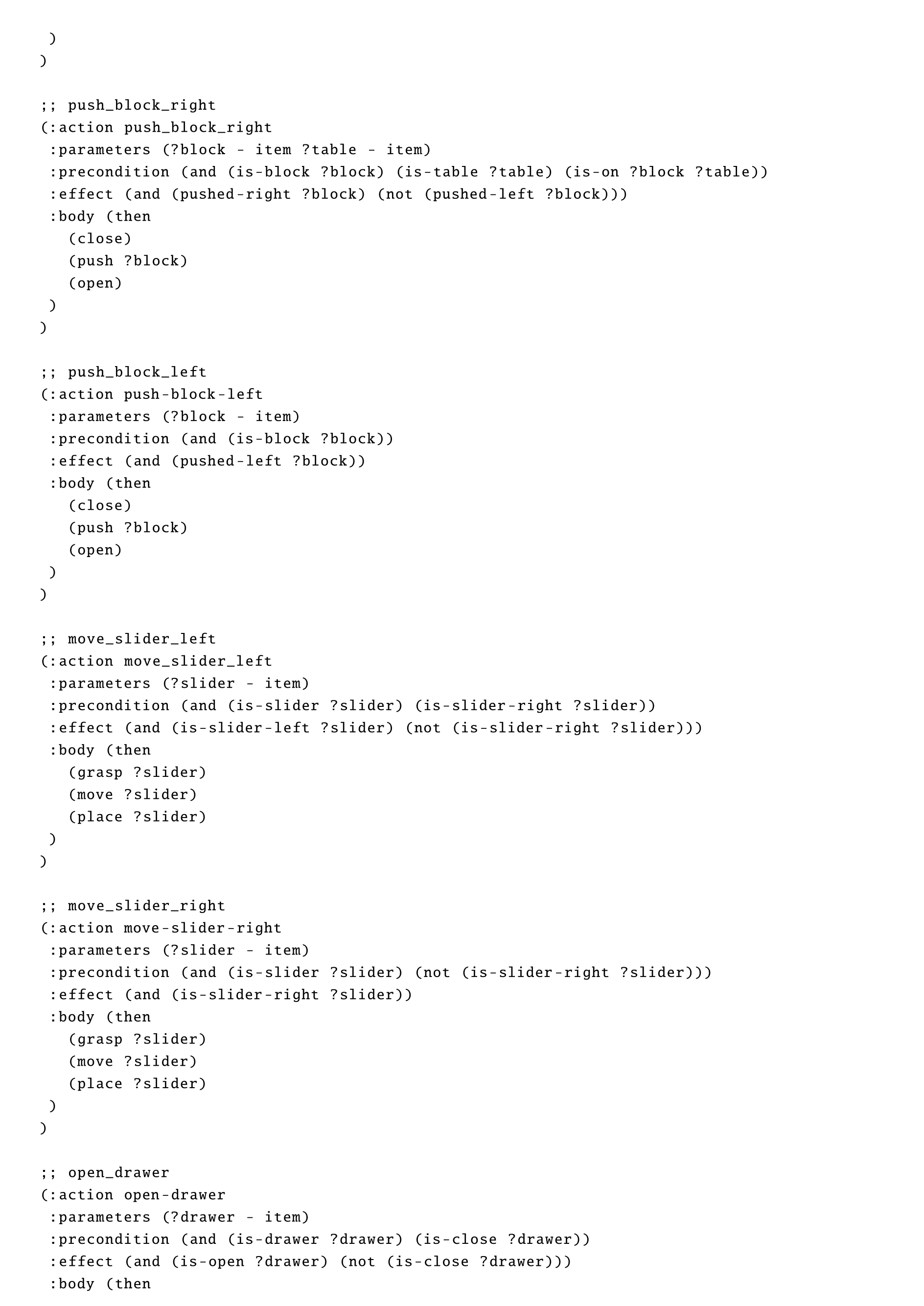
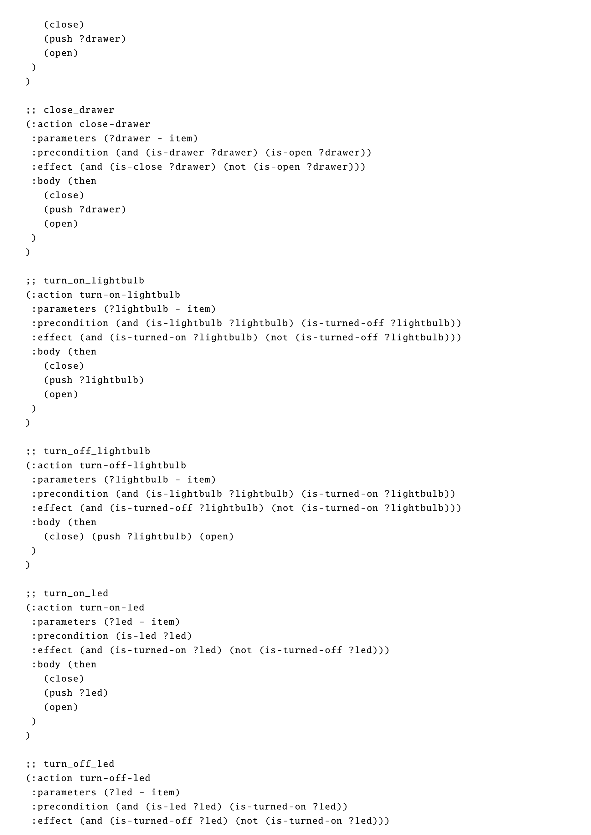
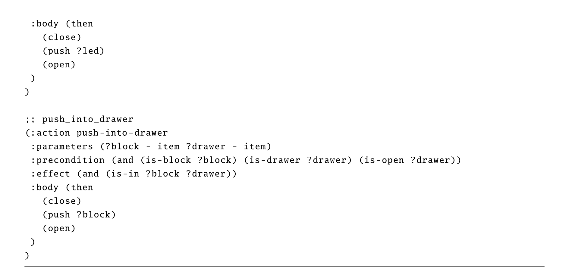
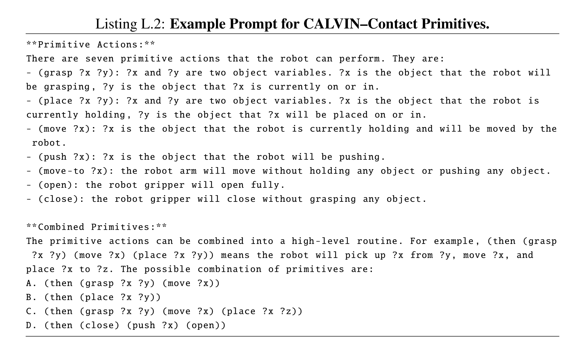
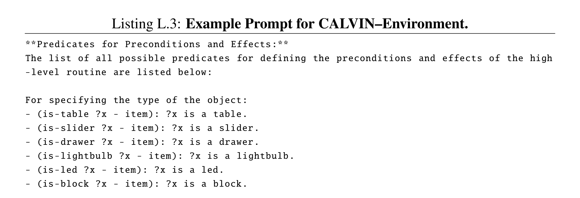
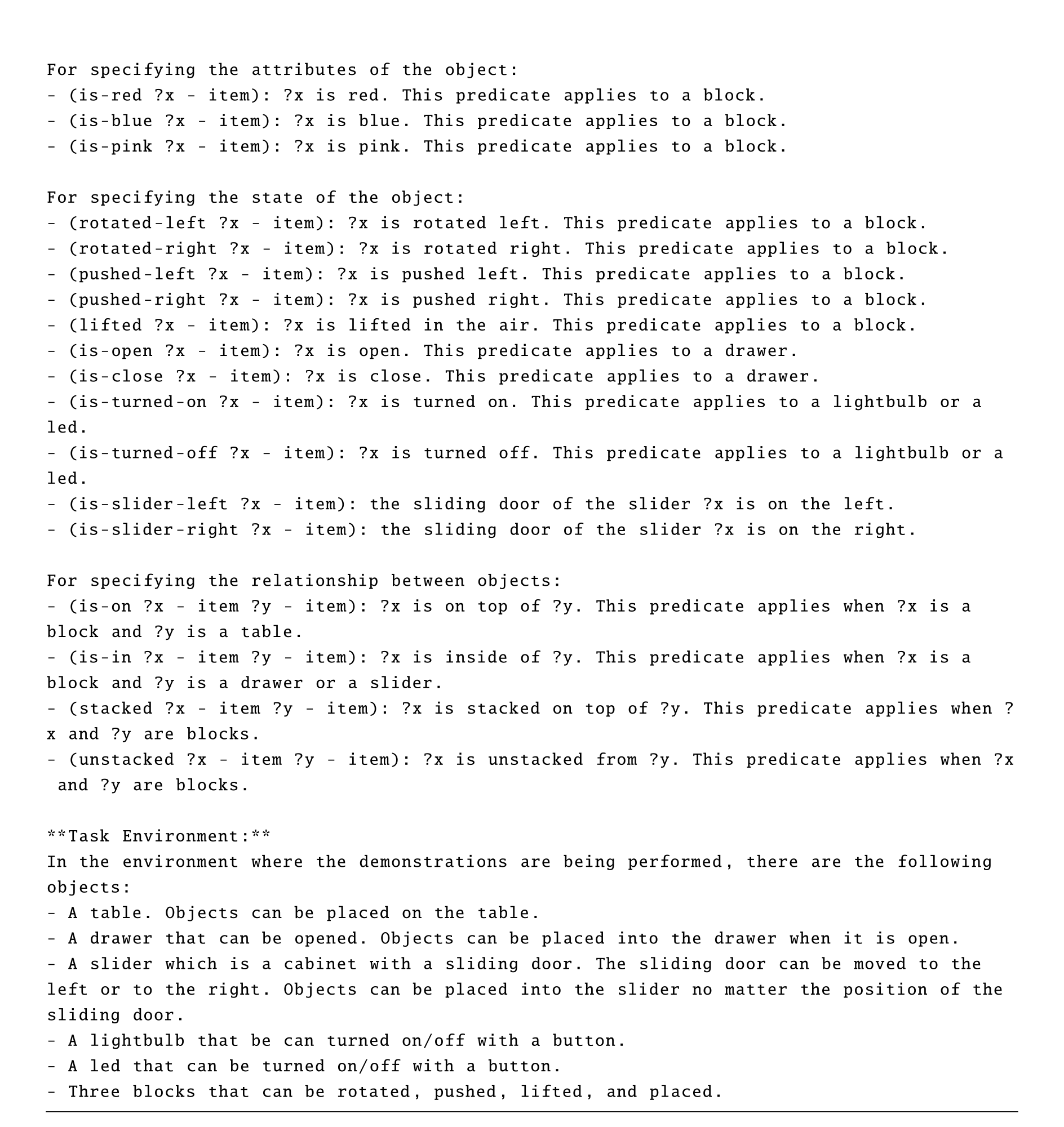
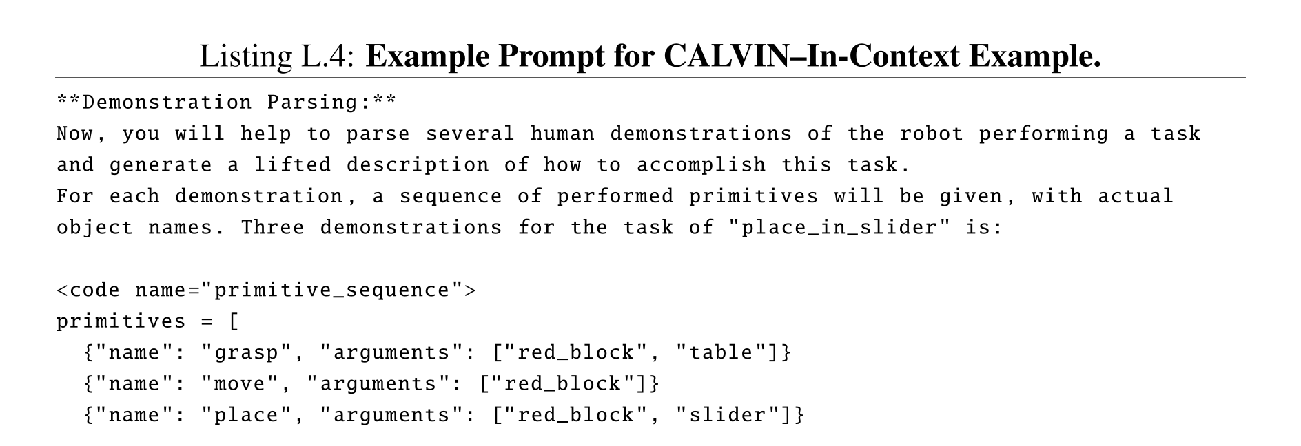
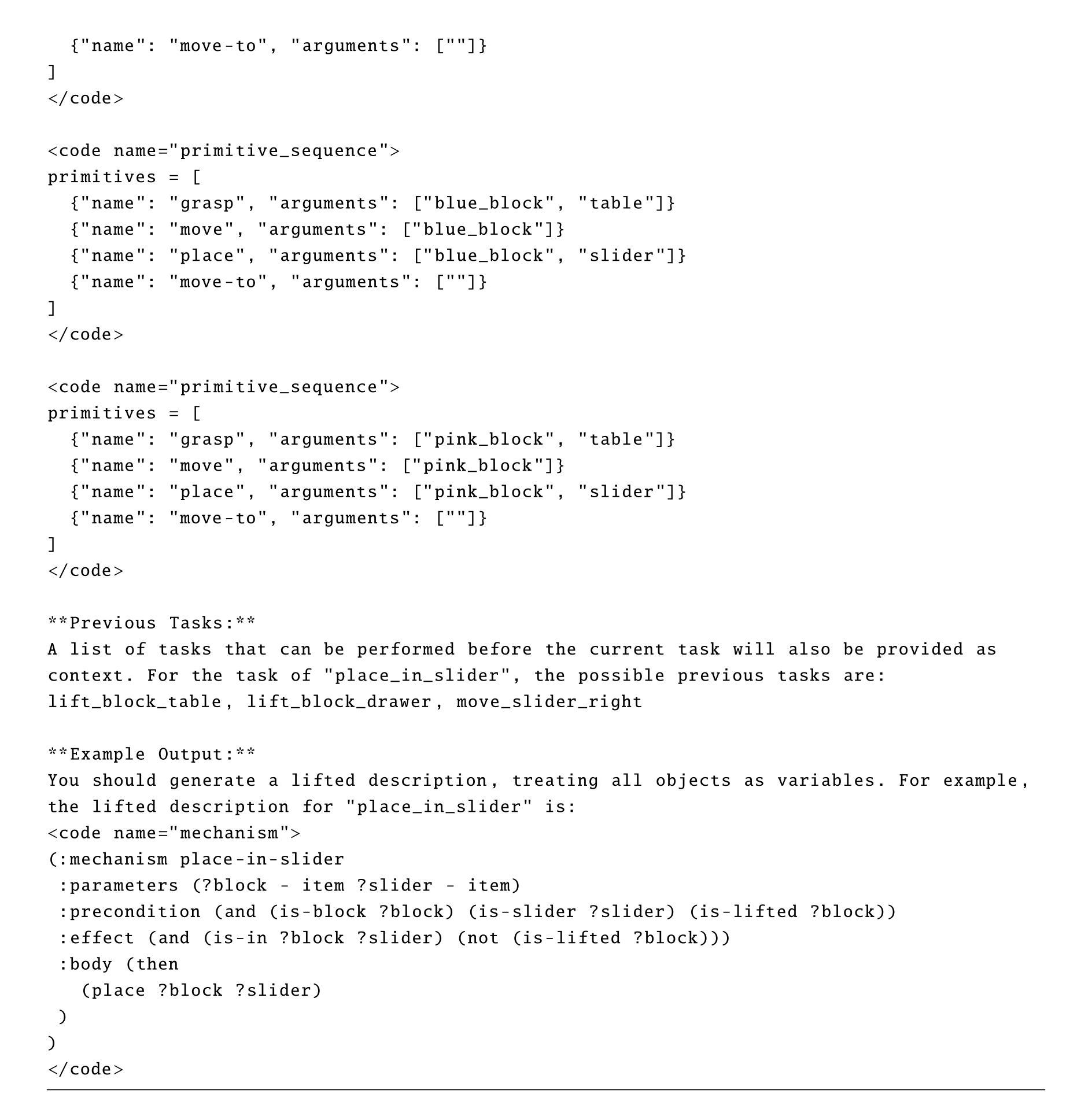
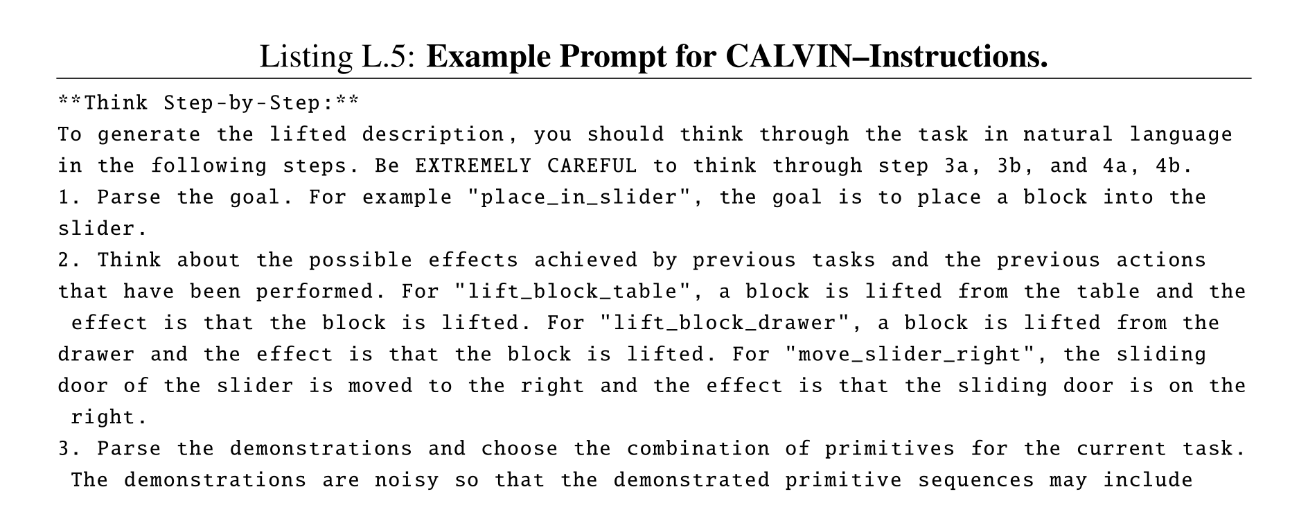

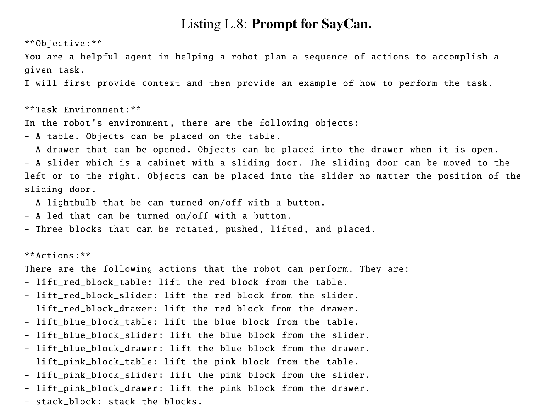
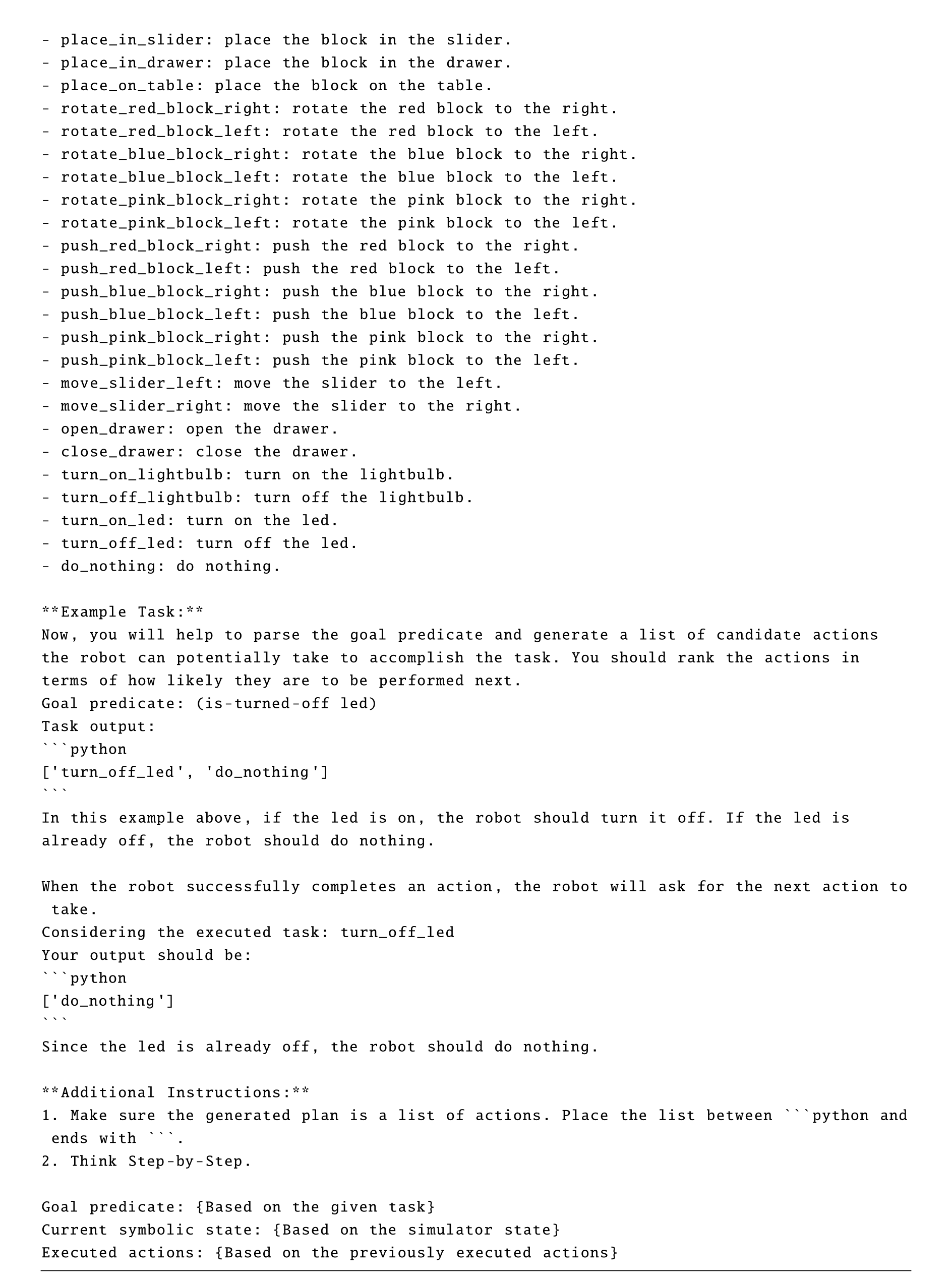

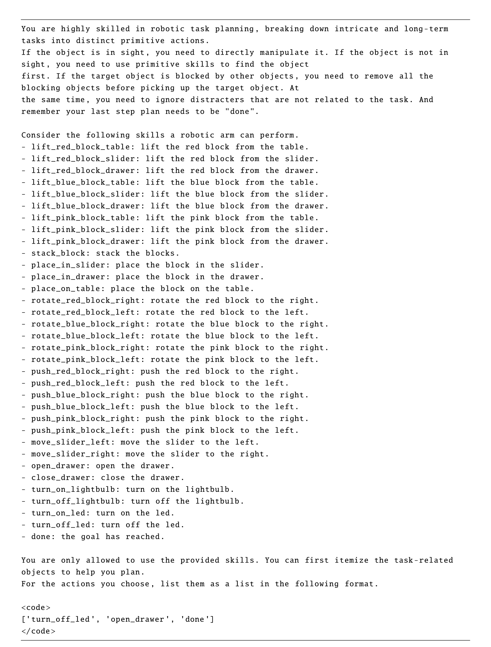


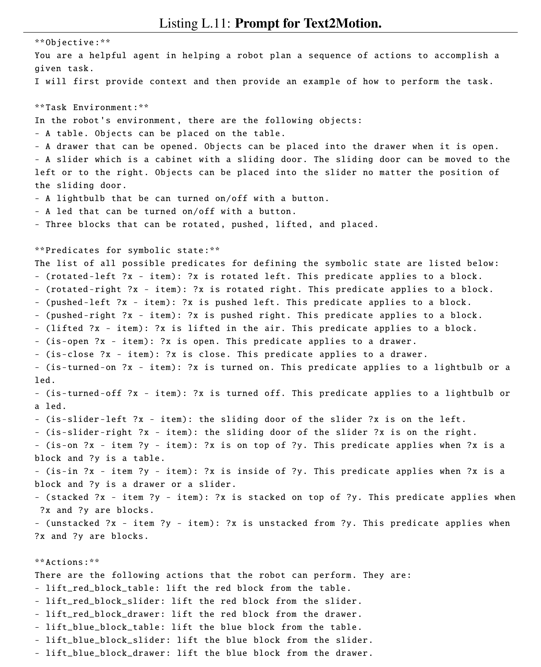
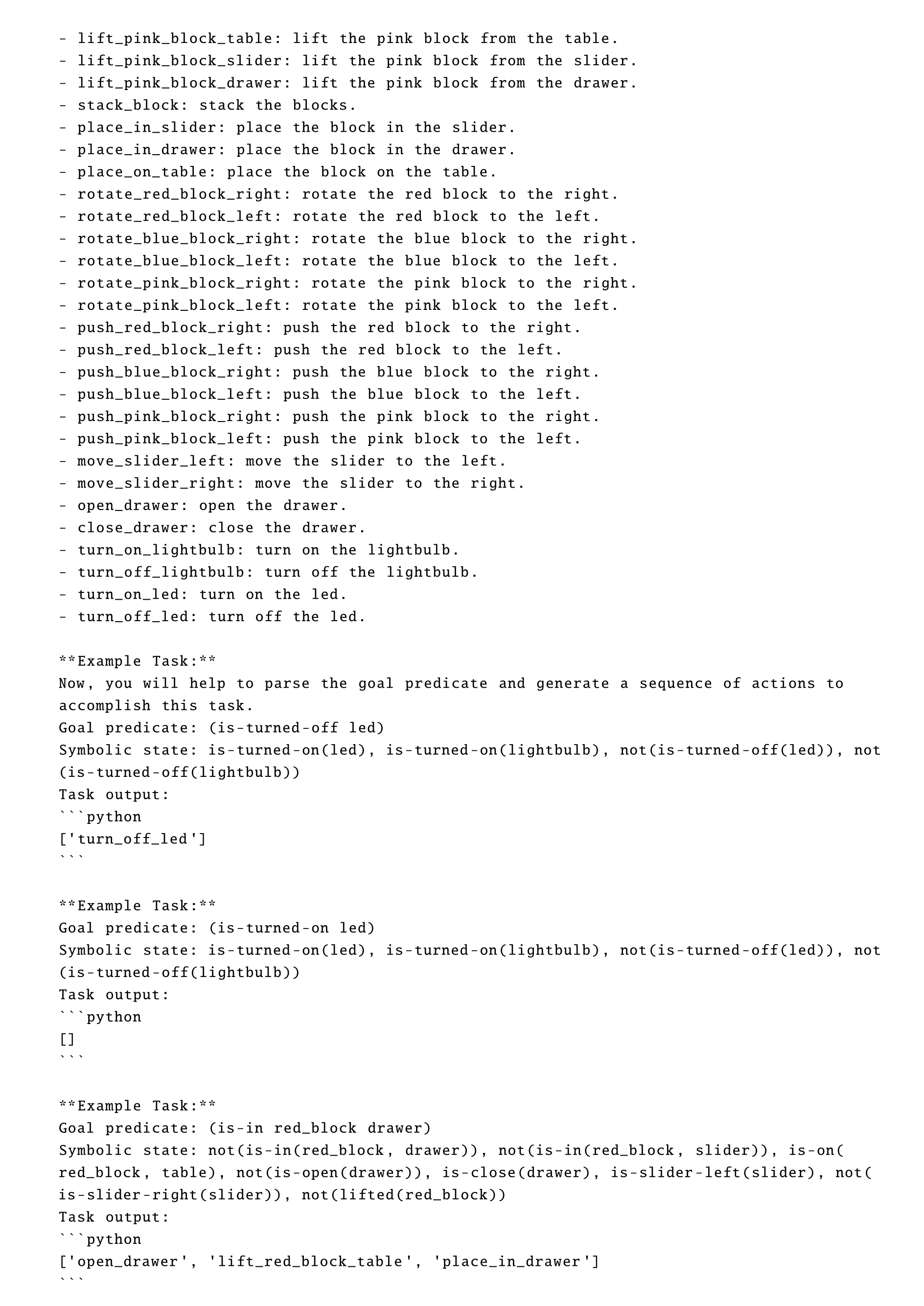
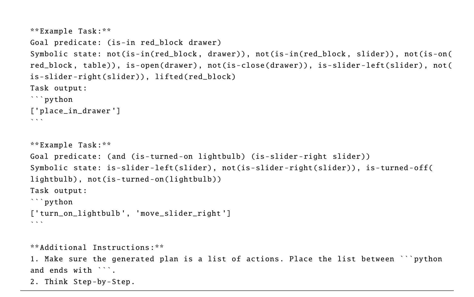
Appendix for Hybrid Imperative-Declarative Action Representations
The appendix defines partial-order refinement, gives the soundness/completeness argument and CSP implementation, qualifies the width analysis, and supplies NAMO and CDL examples. The formal search model and the practical bounded samplers must be distinguished.
Refinements and The Crow Interpreter
Sequential and unordered groups form nested partial orders; tail selects statements that can appear last. Refinement replaces a goal with a matching rule and either serializes its body or merges promotable subgoals for interleaving. Separating the plan generator from assertions/effects makes soundness testing explicit and allows incremental pruning rather than blindly enumerating full plans.


Equation

The Completeness and Soundness of Crow
The proof decomposes refinement into left, middle and right traces, then uses induction and iterative depth limits to argue exhaustive generation. Assertions are checked during refinement or CSP solving. The proof does not remove the earlier caveat that commits can prune necessary alternatives, nor prove completeness of a finite-budget continuous sampler. External correctness still requires accurate modeled effects.
Equations


Formulations and Algorithms for Constraint Satisfaction Problems
Constraints must refer to the state at the time they were generated. Time-indexed fluents turn state-dependent effects into pure equalities over variables, so later feature changes do not alter the meaning of an earlier constraint. Free-variable effect values become new CSP variables linked to their defining functions.


Sampling-based Continuous Constraint Satisfaction Problem Solver
The solver propagates forced Boolean assignments, evaluates functions whose inputs are known and discards unused return variables. It searches discrete assignments before continuous ones, then calls matching conditional generators. Practical generator outputs are explicitly capped, so failure can mean exhausted sampling rather than proof that no satisfying assignment exists.

Proofs for Planner Complexity
Commit fixes a feasible prefix and its continuous assignments. Strong serialization requires that independently solved optimal subplans remain compatible when concatenated; optimality here is relative to plans expressible by the supplied rules. The N^{O(K)} width statement concerns discrete problems without bind or behavior for-loops. The text varies between counting accumulated middle/right goals and middle goals, so it should not be read as a precise unconditional runtime bound for the full implementation. Hybrid extrapolation assumes a suitable bound on continuous CSP difficulty.
Implementation Details for NAMO
The full NAMO program chooses a waypoint and connecting path, interleaves reaching that waypoint with clearing blockers, and uses lower-level rules to approach, attach, move and detach objects. Generators use grid A* with different collision assumptions; candidate obstacle placements initially ignore robot reachability and are checked through subsequent constraints. Crucially, all compared algorithms are capped at one intermediate waypoint. The experiments therefore test a bounded implementation of the more general language.
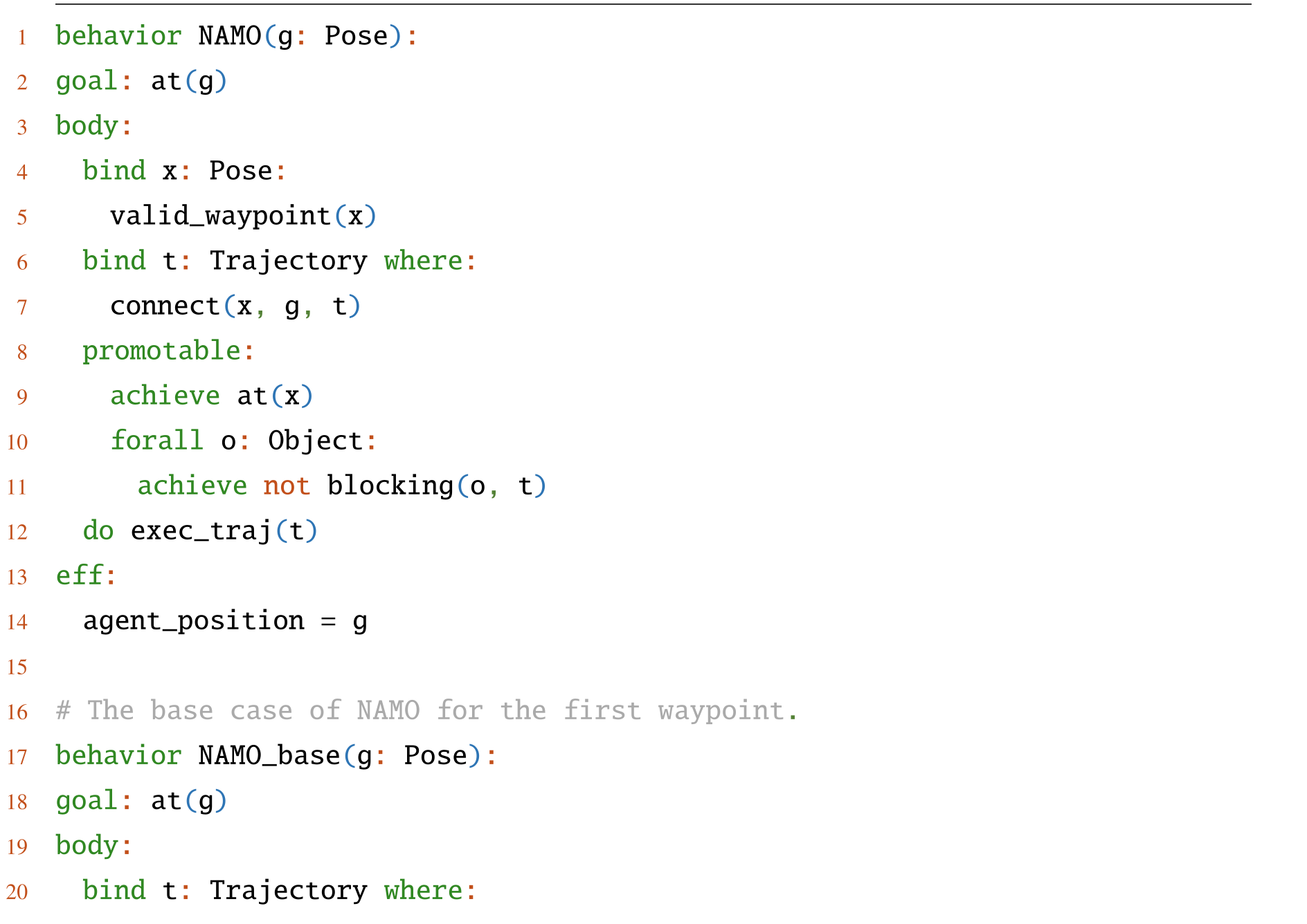
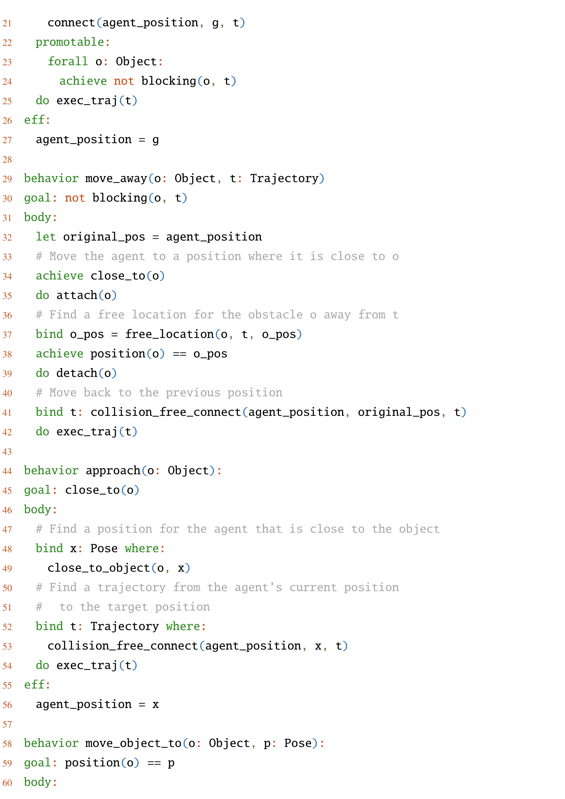

Manual of CDL
The manual explains typed object-centric state, finite computation graphs, external functions/generators and effect compilation, followed by cupboard and blocks-world examples. These listings document representational possibilities rather than a fully validated software package.
Key Concepts
Lifted features and behaviors reuse definitions across entities. Data-oblivious computations have an input-size-dependent finite graph, enabling parameters to remain symbolic while controller structure is constructed. Bounded loops and conditionals can be expanded; value-dependent unbounded while loops are excluded from this subset. External black-box functions remain outside those restrictions.




State Representation: Types and Features
Objects and values have distinct types; quantification ranges over the finite entity set, not arbitrary infinite value domains. New/deleted objects can be represented through preallocated hypothetical entities and deletion flags, which requires a known creation bound. Features map finite tuples of typed entities to scalar, vector or external Python values.





Functions
Primitive functions are externally implemented; derived functions compose feature reads, finite quantifiers, arithmetic, local assignments, conditionals and parallel object loops. Direct or indirect self-recursion is prohibited for derived function bodies to preserve a finite data-oblivious computation graph.



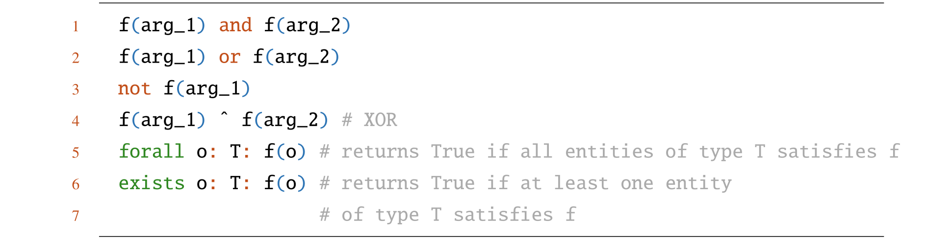



Non-Data-Oblivious Functions and Generators
External functions can perform sophisticated non-oblivious computation. Generators provide conditional inverses: given selected inputs, they propose outputs satisfying a declared relation. A generator’s declared guarantee depends on its actual implementation; the syntax alone cannot establish physical feasibility or completeness.
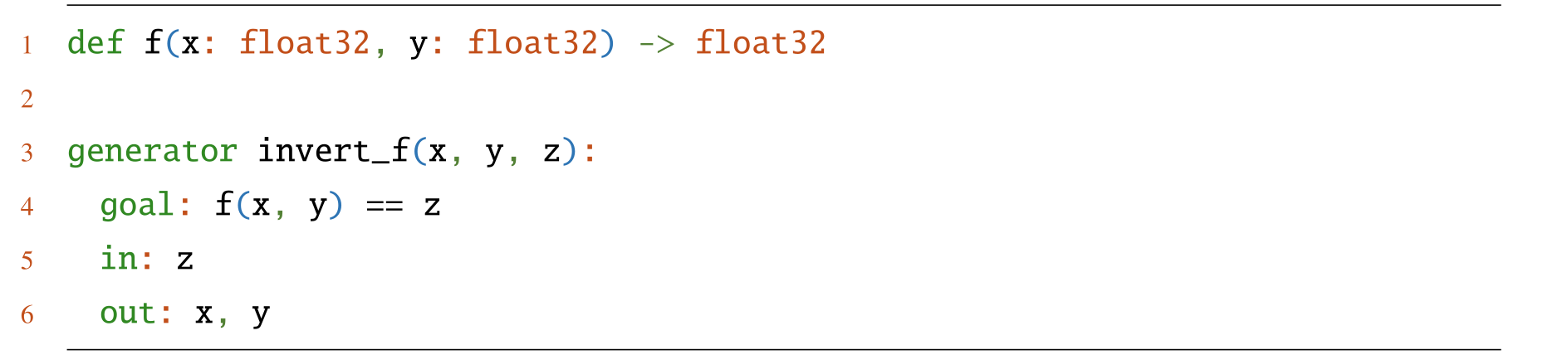
Behavior Effects
Finite data-oblivious effect programs can be expanded into logical descriptions of their state updates, allowing constraint-based or backward reasoning in addition to forward execution. The bounded three-step decrement example illustrates conditional unrolling. This compilation describes the supplied transition program; it does not verify that program against physical reality.
Equation

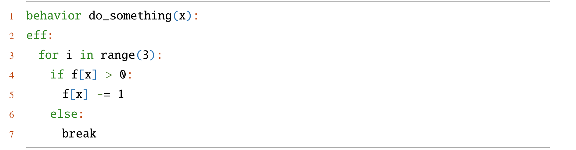
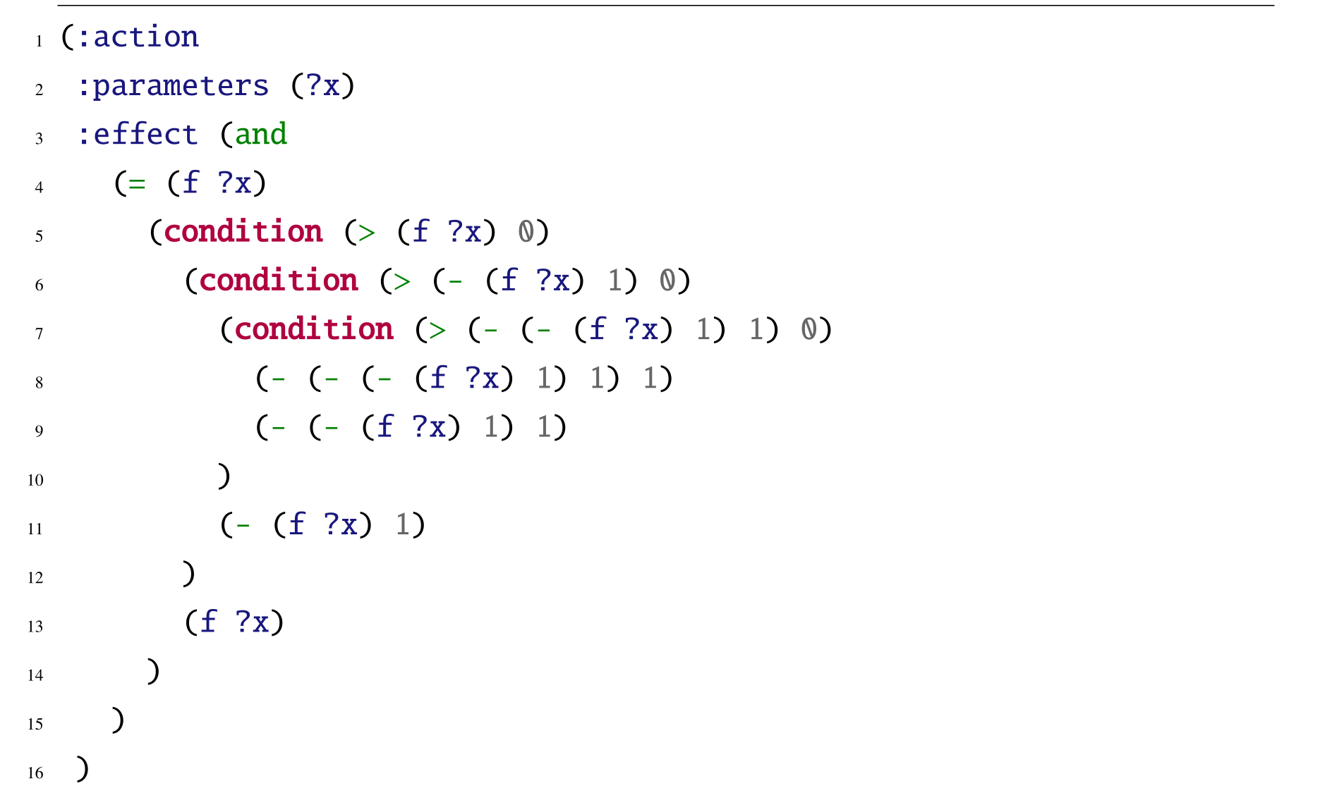

Examples
The cupboard example mixes unordered prerequisites with subsequent ordered placement. Blocks-world rules and Figure M-1 illustrate interleaving needed for the Sussman anomaly. Source listings contain an apparent error: after unstack(x,y), the holding-from-stack rule assigns holding[y] rather than holding[x]. Figure M-1’s prose also repeats on(A,B) where the remaining top-level goal is on(B,C). Preserve these source artifacts and treat them as illustrative notation, not a proven runnable implementation.
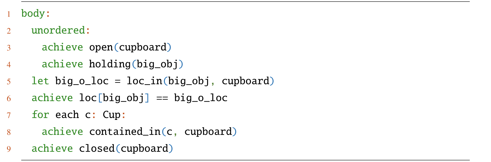
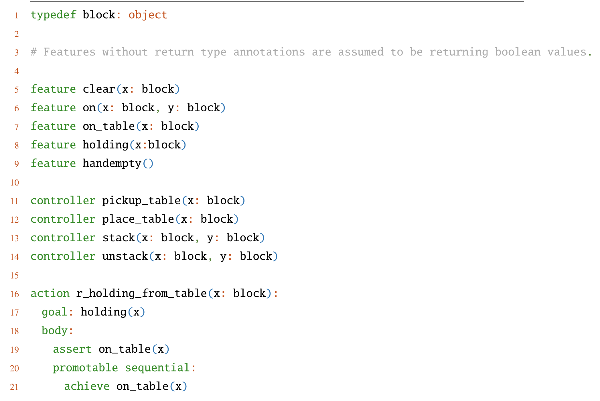
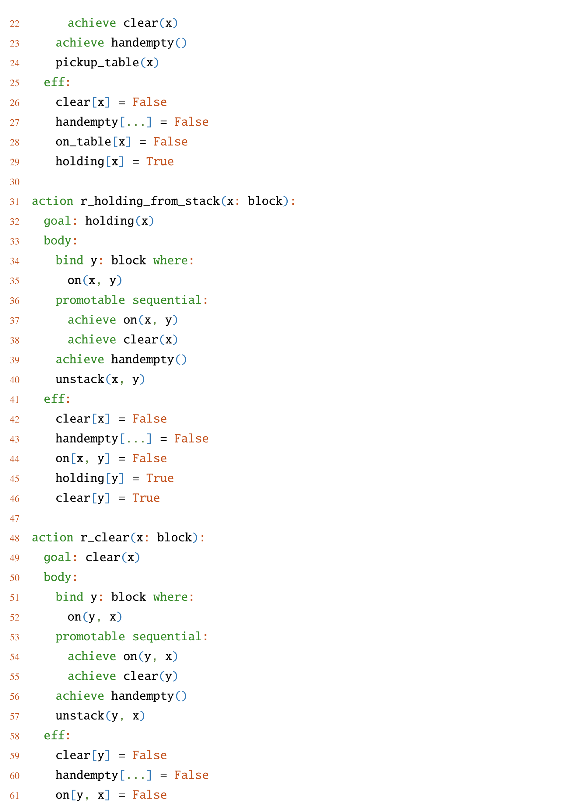
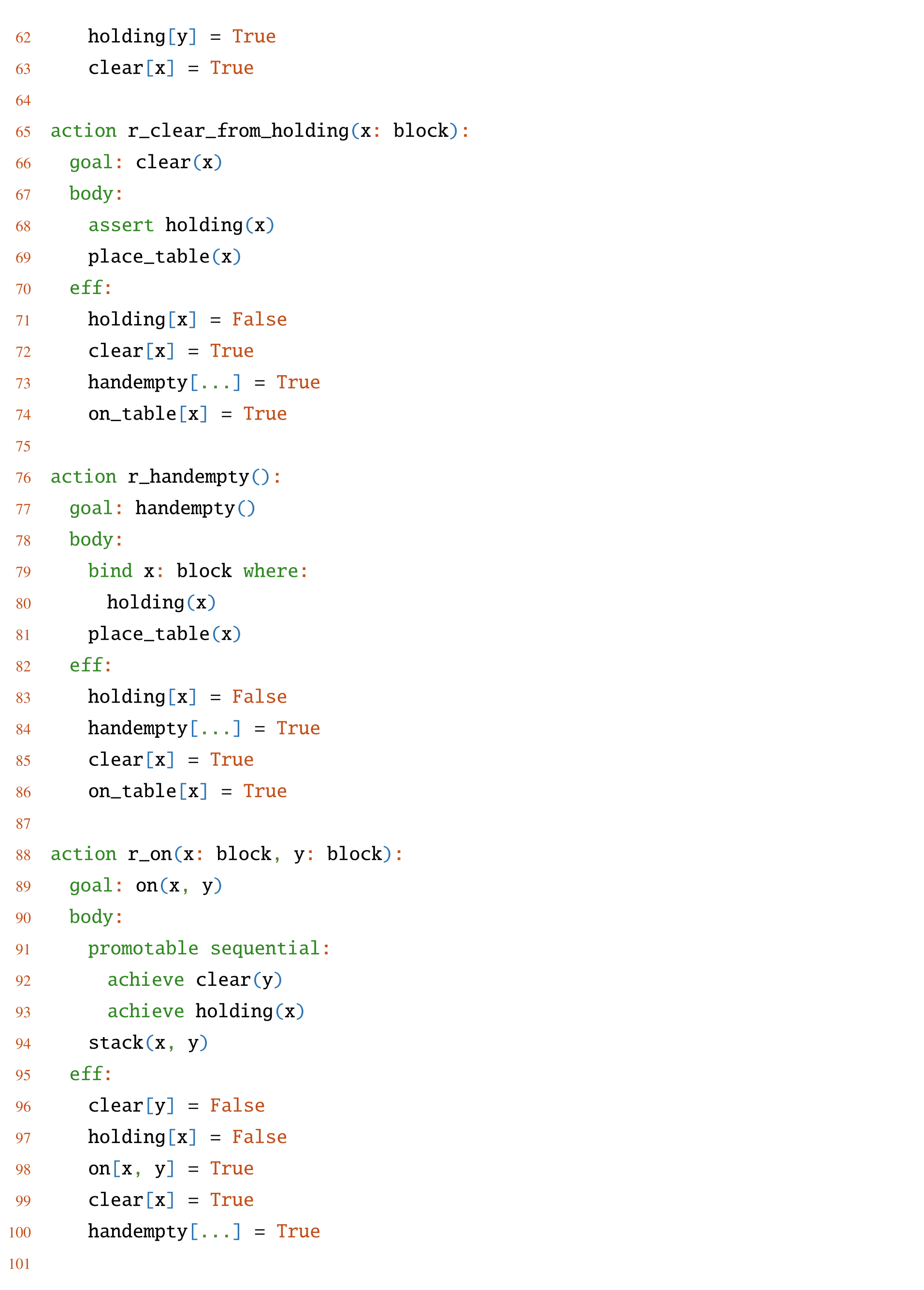
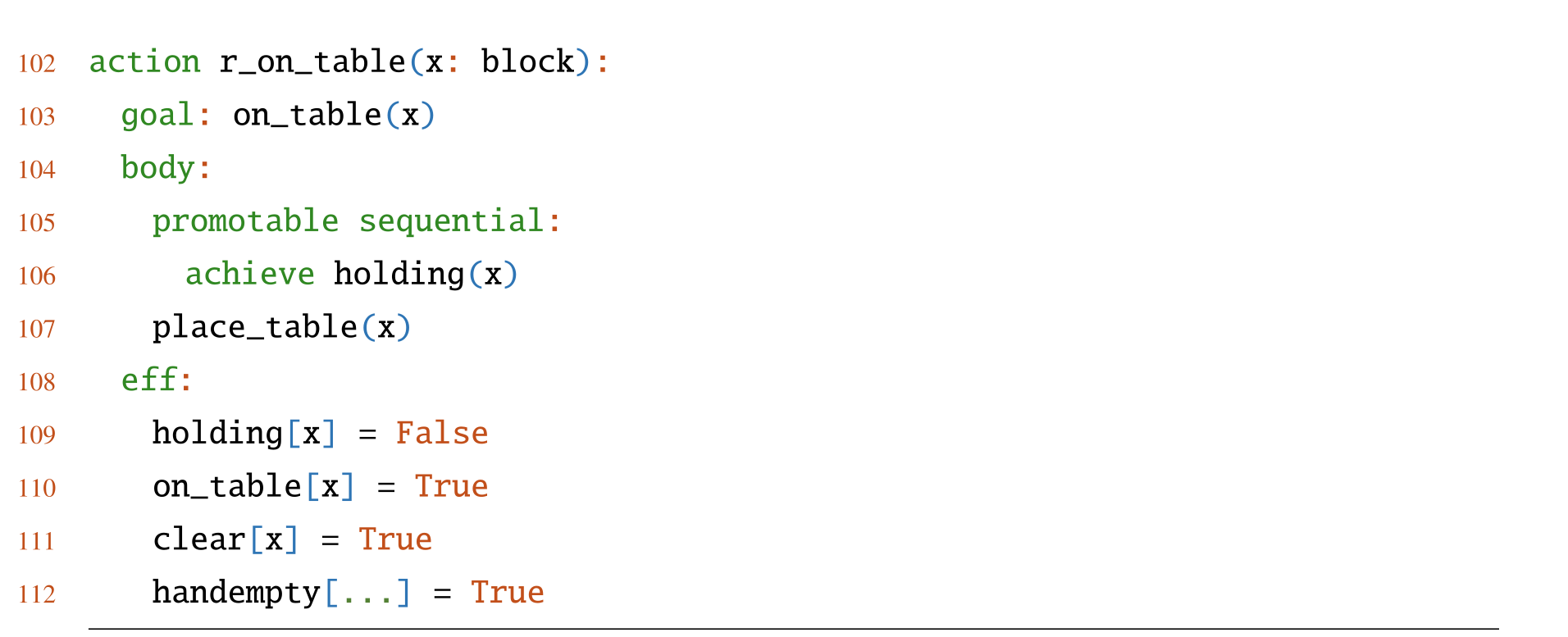
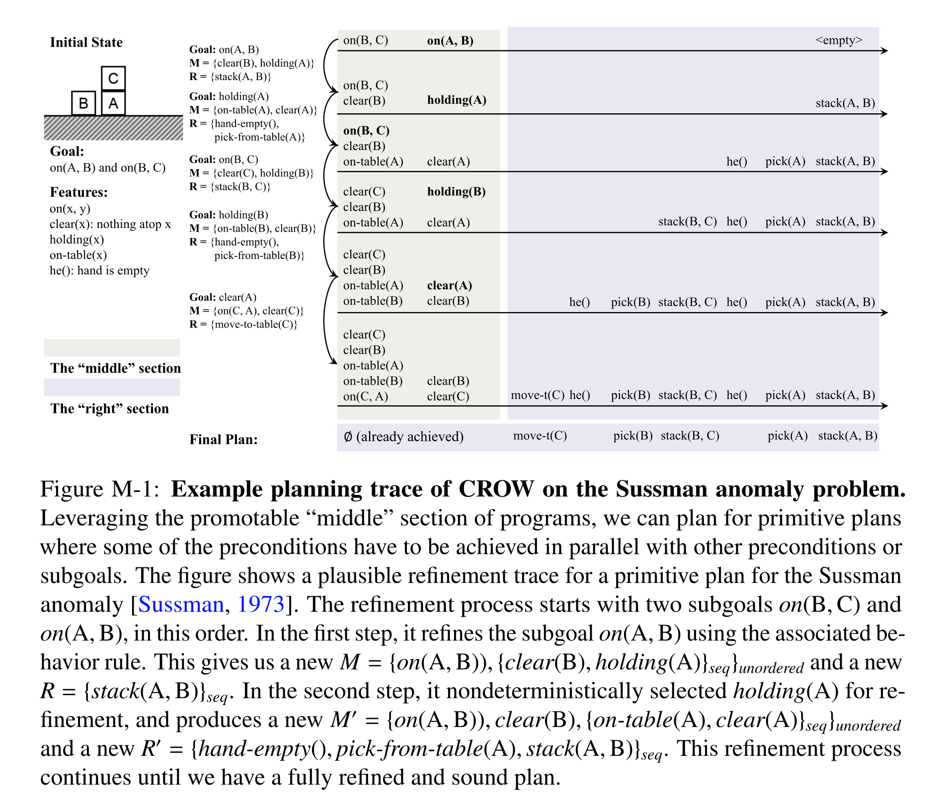
Figure M-1: Example planning trace of CROW on the Sussman anomaly problem. Leveraging the promotable “middle” section of programs, we can plan for primitive plans where some of the preconditions have to be achieved in parallel with other preconditions or subgoals. The figure shows a plausible refinement trace for a primitive plan for the Sussman anomaly [Sussman, 1973]. The refinement process starts with two subgoals on(B, C) and on(A, B), in this order. In the first step, it refines the subgoal on(A, B) using the associated be- havior rule. This gives us a new M = {on(A, B)), {clear(B), holding(A)}seq}unordered and a new R = {stack(A, B)}seq. In the second step, it nondeterministically selected holding(A) for re- finement, and produces a new M′ = {on(A, B)), clear(B), {on-table(A), clear(A)}seq}unordered and a new R′ = {hand-empty(), pick-from-table(A), stack(A, B)}seq. This refinement process continues until we have a fully refined and sound plan.
Original linked resources
The original dissertation links these project pages, implementations and related resources.
- https://en.wikipedia.org/wiki/Closed-world_assumption
- https://en.wikipedia.org/wiki/Inversion_(discrete_mathematics)
- https://sites.google.com/view/neural-logic-machines
- https://research-football.dev/
- https://concepts-ai.com/p/mechanisms
- https://github.com/haosulab/MPlib
- https://en.wikipedia.org/wiki/Chernoff_bound#Multiplicative_form_(relative_error)
- https://github.com/concepts-ai/goal-regression-width
- https://raw.githubusercontent.com/brendenlake/SCAN/master/simple_split/tasks_train_simple.txt
- https://raw.githubusercontent.com/brendenlake/SCAN/master/simple_split/tasks_test_simple.txt
- https://raw.githubusercontent.com/brendenlake/SCAN/master/add_prim_split/tasks_train_addprim_jump.txt
- https://raw.githubusercontent.com/brendenlake/SCAN/master/add_prim_split/tasks_test_addprim_jump.txt
- https://raw.githubusercontent.com/brendenlake/SCAN/master/template_split/tasks_train_template_around_right.txt
- https://raw.githubusercontent.com/brendenlake/SCAN/master/template_split/tasks_test_template_around_right.txt
- https://raw.githubusercontent.com/brendenlake/SCAN/master/length_split/tasks_train_length.txt
- https://raw.githubusercontent.com/brendenlake/SCAN/master/length_split/tasks_test_length.txt
- https://github.com/google-research/google-research/tree/master/saycan