At a glance
This preprint compares digit decoding from human stem-cell-derived neural cultures across cell lineages, physical architectures, and analysis pipelines. Artifact-controlled frequency-domain decoding averages 39.3% accuracy, versus 14.0% for spike counts with held-out trials. Modular cortical cultures perform best in the main comparison. Including stimulation artifacts or holding out time bins instead of trials can substantially inflate apparent accuracy. These are reservoir readout experiments, not evidence that cultures learned digit recognition through feedback.
1 Introduction
Synthetic Biological Intelligence studies how living neural networks transform information. Reservoir computing uses their dynamics as a feature generator and trains a separate readout. Comparing cultures requires controlling cell identity, geometry, stimulation artifacts, and evaluation splits.
Here, an artificial spiking autoencoder converts MNIST images into electrical stimulation patterns delivered through the CL1 platform. Identical recordings are evaluated with frequency-domain and spike-count readouts, using shuffled-label, saline-only, and synthetic-spike controls. The study asks which combinations produce reliable decodable responses.
Related references: [1], [2], [3], [5], [6], [8], [9], [11], [12], [13], [16], [17], [20], [21], [23], [24], [25], [26], [27], [28], [29], [30], [31], [32], [33], [7], [34], [35], [37], [38], [40], [39].
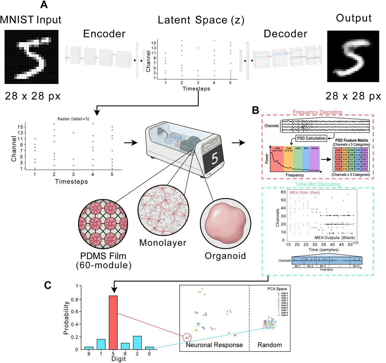
A Conversion of MNIST digit to spatiotemporal spike-train signal via a spiking autoencoder. An image (28 × 28 pixels) was fed into a multi-layered convolutional neural network (CNN) with leaky integrate-and-fire (LIF) neurons. The latent space of the autoencoder was constructed to represent a spatio-temporal spike-train, validated by reconstruction of the image via a decoder. After training the autoencoder for 100 epochs, a reconstruction loss of ~0.2 was achieved. The latent space of the final epoch was then presented as a sequence of stimulations to a CL1 containing cell cultures on microelectrode arrays (MEAs), in a spatio-temporal MNIST classification task with different neuronal culture setups (PDMS Film 60-module, Monolayer and Organoid). B Different decoding mechanisms - Frequency (red) and Time-Bin (cyan) based decoding. C Classification of the predicted digit after decoding, and an example PCA space (1st and 2nd PCs) for Neural responses allowing for higher classification accuracy than Random responses.
2 Results
2.1 Generating Neural Cultures
Human induced pluripotent stem cells were differentiated into cortical or hippocampal lineages and grown as unstructured monolayers, 60-module microfluidic networks, or three-dimensional organoids. Morphology, immunostaining, and gene expression confirm relevant lineage markers. The design compares six culture configurations, with unequal group sizes.
Related references: [41], [17], [42], [44].
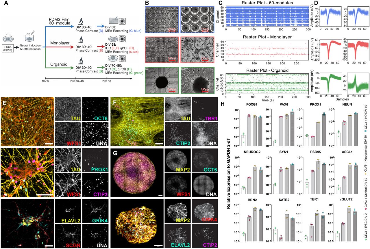
A: Schematic illustration of differentiation, plating and recording protocol for each cell structure (60-module device in blue, Monolayer in red, Organoid in Green). Letters in the schematic refer to subplot headings in the current figure. B: Microscope images of Top: Modular PDMS Film 60-module device. Each well is connected only to its eight closest neighbors via micro-fluidic channels which encourage axonal growth from well to well. Middle: Monolayers. Bottom: Organoids. C: Example 5 minute raster plots for each structure type. D: Example waveforms (3 ms cut-out). E: Immunostaining analysis after long-term culture shows matured TAU+ neurons constituting distinct hippocampal subfield fates: OCT6 and WFS1 (CA1), CTIP2 (CA1 and DG), PROX1 (DG), ELAVL2, GRIK4 and SCGN (CA3). Scale bar is 50 µm. F: Immunostaining analysis after long-term culture shows matured TAU+ neurons constituting CTIP2+ (cortical layer V) and TBR1+ (cortical layer VI). Scale bar is 100 µm. G: Immunostaining analysis of Hippo Organoids shows matured MAP2+ neurons constituting distinct hippocampal subfield fates: OCT6 and WFS1 (CA1). Scale bar is 50 µm. H: qRT-PCR confirms the expression of proneural markers and markers of cortical and hippocampal neurons at DIV 60 (n = 3 independent experiments each, data are mean ± SEM).
2.2 Electrophysiology and Criticality
Architecture and lineage affect firing rates, inter-spike intervals, avalanche statistics, and criticality measures. Modular hippocampal cultures show high activity and short intervals; hippocampal organoids have a distinctive dynamical profile. Activity metrics are correlated, so they cannot be treated as independent explanatory factors. A single criticality score does not establish computational superiority.
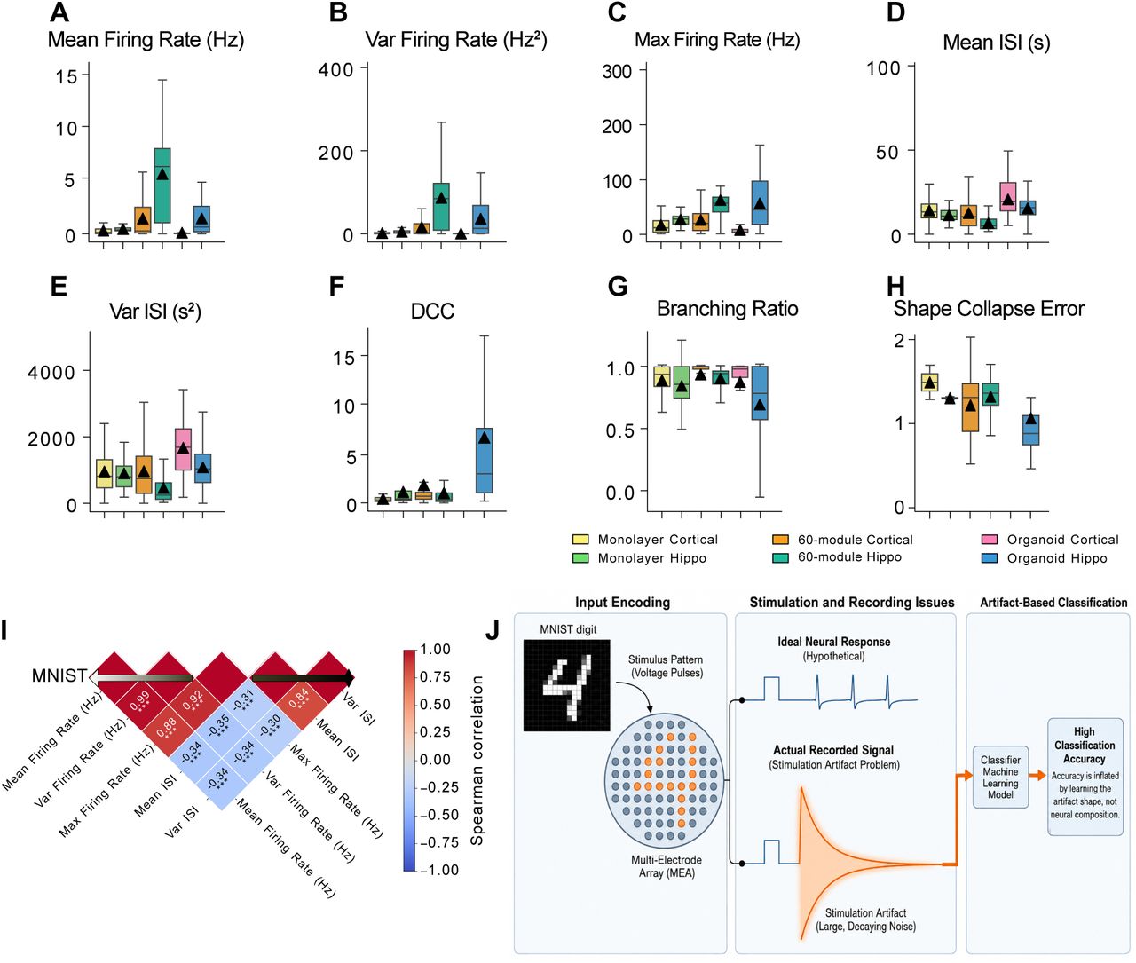
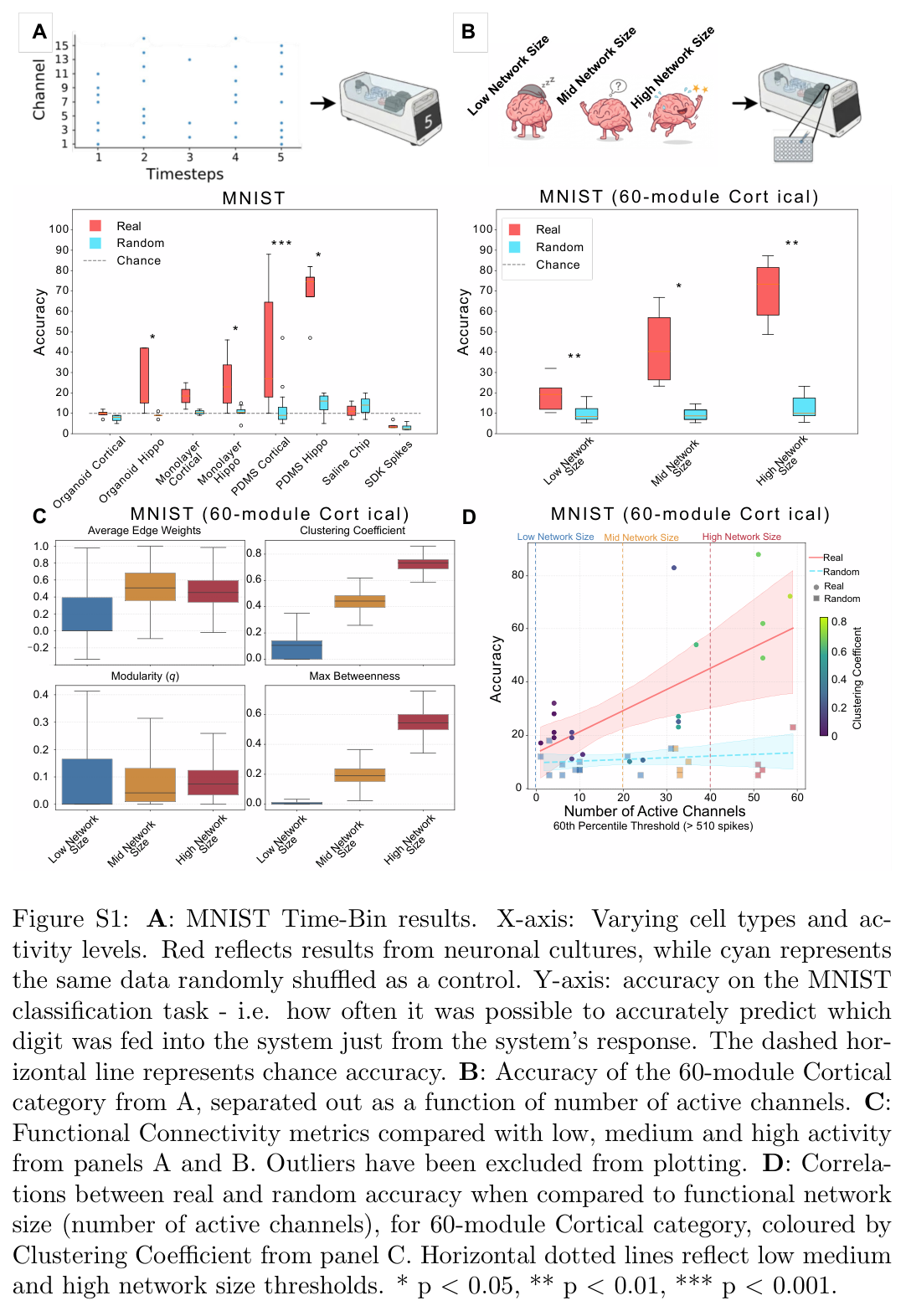
Spontaneous culture-level activity is compared across diverse cellular configurations using boxplots. Culture ages ranged from DIV 58 for Monolayers to up to DIV 80 for Organoids. A total of 53 cultures were recorded both baseline (spontaneous) and playing MNIST (see Supp Table S1 for full details). (A–C) Spiking statistics, including Mean Firing Rate, Variance of Firing Rate, and Maximum Firing Rate. (D,E) ISI metrics, showing Mean and Variance of ISI. (F–H) Network criticality metrics, specifically the DCC, Branching Ratio and Shape Collapse Error. For all plots, boxes represent the interquartile range (IQR) and median, whiskers extend to 1.5×IQR, and black triangles denote the mean. The metrics highlight distinct spontaneous activity profiles, demonstrating elevated activity and near-critical dynamics in modular networks compared to unstructured monolayers and organoids. I Heatmap comparing correlations in electrophysiological activity during the MNIST task. J Neuronal activity can be masked by stimulation artifacts if not properly blanked. This affects both functional connectivity of the cultures as well as classification accuracy.
2.3 Functional Connectivity
Functional connectivity is estimated from correlations between one-second spike-count bins, retaining connections with absolute correlation at least 0.4. Graph statistics quantify edge strength, clustering, modularity, and betweenness. Hippocampal identity and physical modular confinement often produce stronger local organization; these correlation graphs do not directly measure anatomical synapses.
Related references: [45].
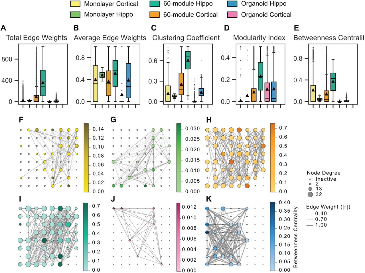
Culture-level network graph metrics are compared across diverse cell configurations using boxplots with overlaid individual data points (A–E). Functional connectivity was measured as thresholded Pearson correlations (|r| ≥ 0.4) between electrodes. Boxes show the interquartile range and median, whiskers indicate 1.5×IQR, and black triangles denote the mean. (F–K) Representative spatial functional connectivity maps for each culture category. Nodes represent active electrodes, with size indicating node degree and color mapping to betweenness centrality. Edge thickness reflects connection weight, illustrating the distinct topological integration and hub formations specific to each architecture.
2.4 Stimulation Artifacts and Classification Errors
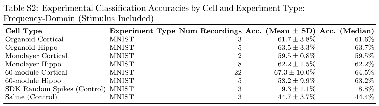
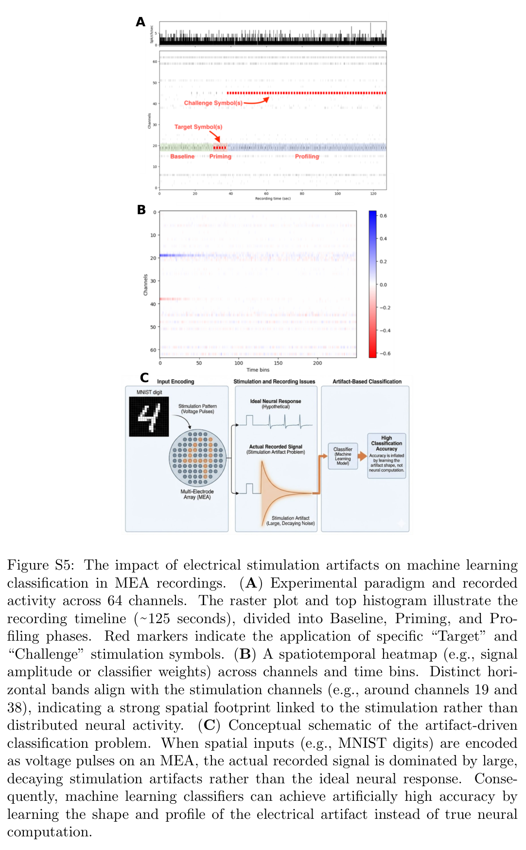
Electrical stimulation leaves large voltage transients that a classifier can decode even without neurons. The main analysis combines hardware/software blanking for two milliseconds after stimulation with spike sorting. A comparison that retains the stimulation window exposes how residual input artifacts can inflate accuracy.
2.4.1 Importance of proper controls
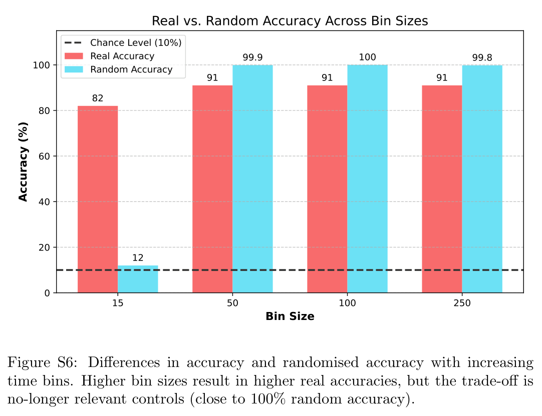
High-dimensional readouts can separate random data when feature counts overwhelm the available observations. The study uses regularization, constrained binning, shuffled labels, saline dishes without cells, and simulated spikes to test for spurious decoding. Some inadequately controlled settings approach perfect accuracy despite lacking a valid neural signal.
Related references: [46].
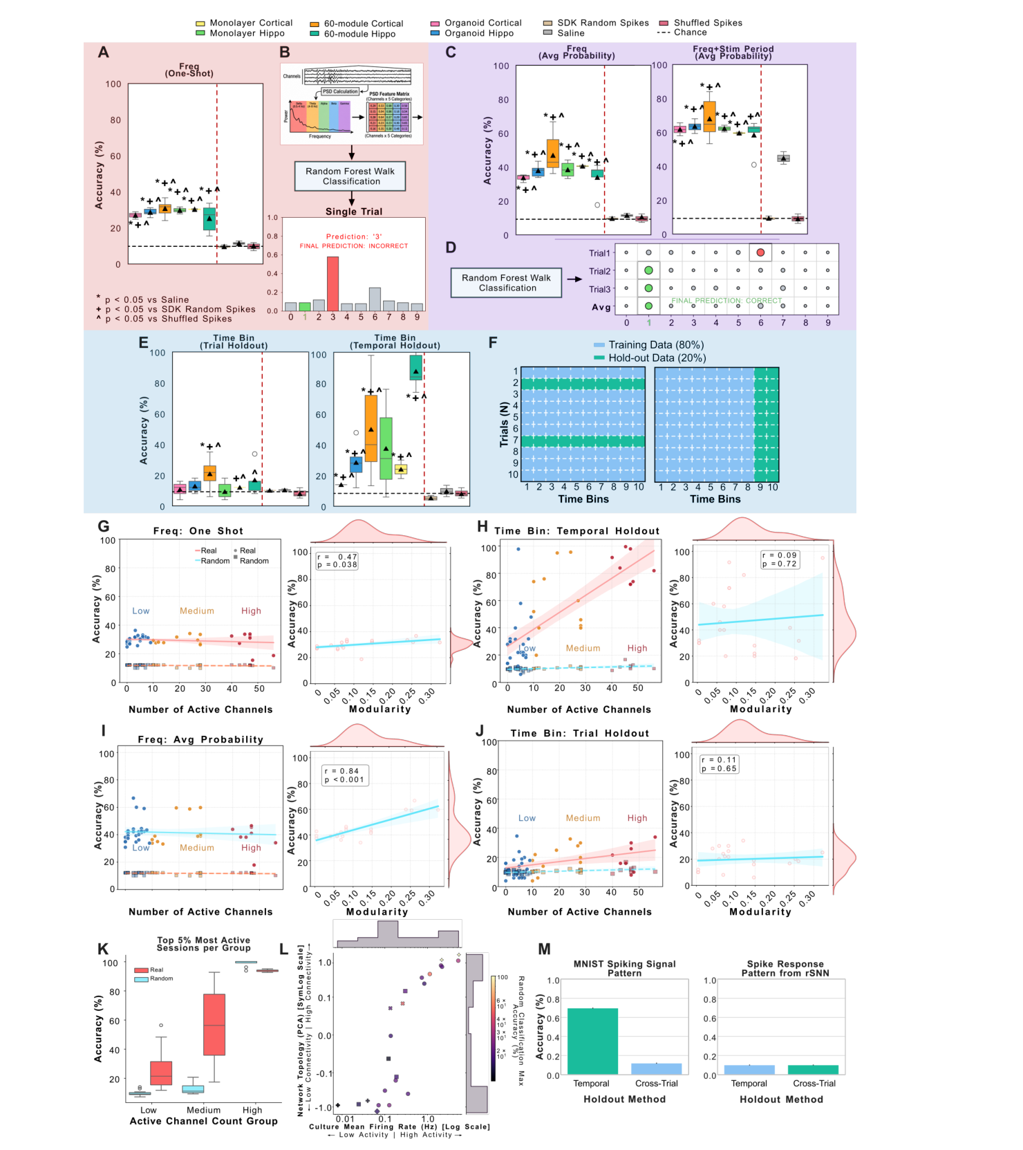
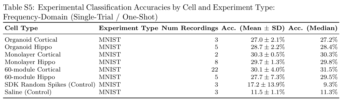
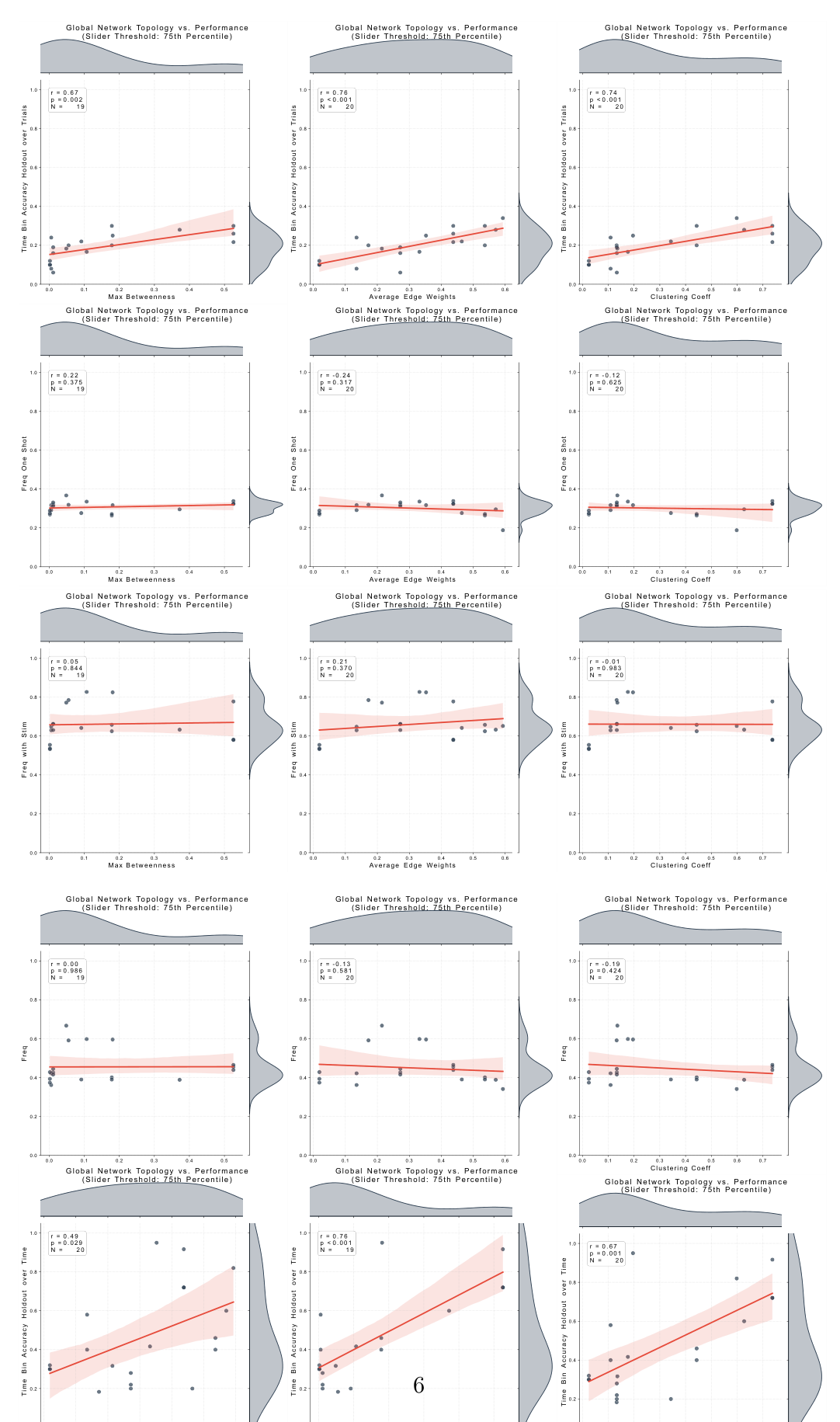
(A–B, Red) Frequency-domain one-shot classification per digit trial. A: Accuracy by cell type and controls: Monolayer Cortical (n = 2), Monolayer Hippo (n = 8), 60-module Cortical (n = 22), 60-module Hippo (n = 5), Organoid Cortical (n = 3), Organoid Hippo (n = 5). Dashed lines: horizontal = chance (10%); vertical red = separates neurons (left) from controls (right). B: Calculation schematic. Significance (t-test vs. controls): ∗p < 0.05 vs. Saline; +p < 0.05 vs. SDK Random Spikes; ^p < 0.05 vs. Shuffled Spikes. (C–D, Purple) Multi-trial average probability frequency-domain decoding. C: Results without (left) vs. with (right) the stimulation window. Including the stimulation window drastically alters apparent accuracy and variability; elevated saline control accuracy under “with Stim” indicates partial contamination by stimulation artifacts. D: Multi-trial calculation schematic. (E–F, Blue) Time-bin holdout decoding. E: Trial holdout (left) vs. time holdout (right). F: Train-test split schematics for trial holdout (80% train / 20% test trials; left) and time holdout (80% train / 20% test time bins; right). (G–J) Network activity and modularity comparisons. Activity is operationalized by active channel count (≥ 75% spike ratio; > 1400 spikes): Low (< 10), Medium (10–30), High (> 30). Left panels compare active channels against frequency decoding (G, I) and time-bin decoding (H, J). Right panels show classification accuracy vs. Modularity metric. K: Neuronal vs. randomly shuffled classification accuracy across top 5% low, medium, and high activity groups. L: Network topology (y-axis), culture mean firing rate (x-axis), and random classification accuracy (hue). Higher connectivity and activity produce higher random accuracy due to overfitting and bin misalignment. M: Cross-trial (N -axis) vs. temporal (T -axis) holdout classification accuracy. Left: The stimulation template control (raw MNIST spatio-temporal spike train) drops from 69.7% to 11.9% in Cross-Trial holdout. Right: The rSNN baseline (two RSynaptic neuron layers) maintains stable accuracy across holdouts, demonstrating that biological culture temporal discriminability is unlikely a data-leakage artifact.
2.5 Classification
2.5.1 Comparing Decoding Mechanisms for MNIST Classification
Four pipelines use the same recordings. The principal frequency-domain pipeline extracts power in five bands from a 400-millisecond window starting ten milliseconds after the last pulse and uses a Random Forest with trial-based validation. A second version includes stimulation. Two spike-count pipelines use logistic regression and identical time bins, differing only in whether trials or time bins are held out.
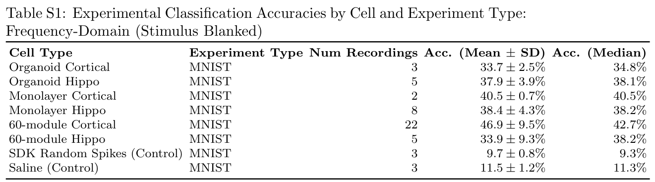
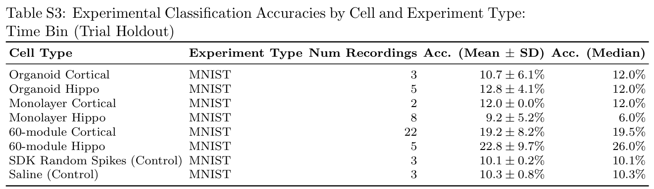
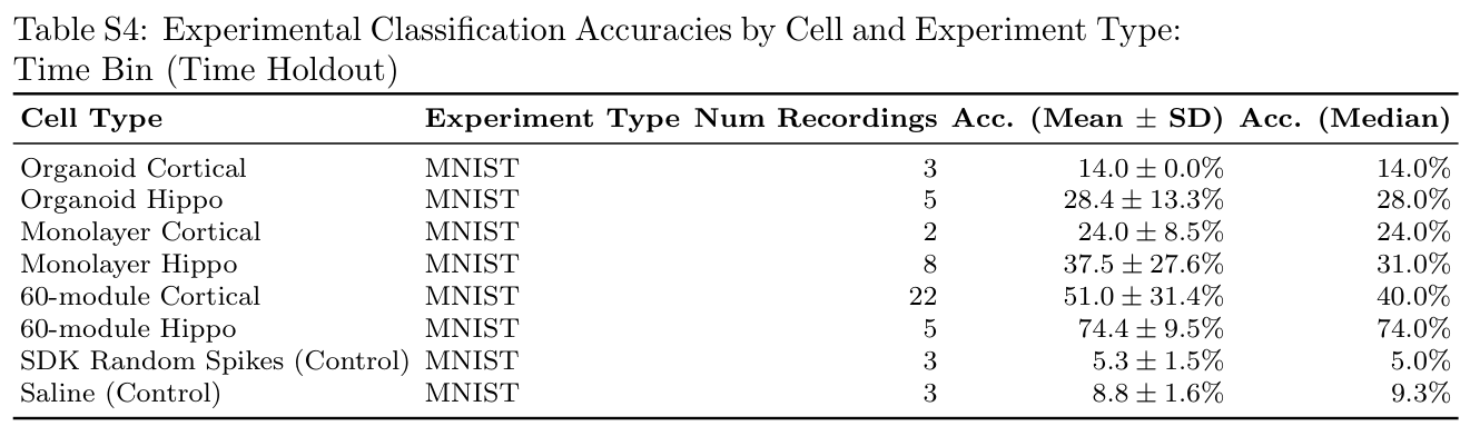
Reported mean accuracies are 39.3% for artifact-controlled frequency features, 14.0% for trial-held-out spike counts, 30.0% for time-held-out spike counts, and 62.5% when stimulation is included. The saline-only control rises to 44.4% with stimulation included, versus 11.3% without it, demonstrating a substantial non-neural contribution to the apparent gain.
Holding out time bins tests predictability within repeated temporal patterns and is not equivalent to generalizing to new trials. Culture rankings also change with the decoder, although modular cortical cultures tend to rank highly. Original figures and supplementary tables preserve the full results.
2.5.2 Comparing Cell Types
With the artifact-controlled frequency pipeline, modular cortical cultures average about 47% accuracy, compared with 34% for modular hippocampal cultures. Hippocampal variants score more highly under temporal holdout, consistent with different persistence or autocorrelation in their responses. That advantage concerns a different prediction problem from trial-held-out classification.
2.5.3 Comparing Cell Structure and Function
Modular cortical cultures have the highest mean frequency-based accuracy, approximately 47%, followed by cortical monolayers at 41% and cortical organoids at 34%. Sample sizes are markedly unequal: 22, 2, and 3 recordings, respectively. These results support an architectural association in this setup, not a general ranking of all biological computing substrates.
2.5.4 Validation of Temporal Holdout
The authors additionally test temporal splits on raw stimulation templates and a simulated recurrent spiking network. Temporal holdout raises template accuracy from 11.9% to 69.7% but does not improve the simulated-network control. They interpret the biological results as reflecting persistent temporal structure. These controls do not make within-trial temporal prediction interchangeable with held-out-trial digit classification.
Related references: [47].
2.5.5 Biophysical Determinants of Reservoir Performance
Moderation Analysis of Network State
Among seven tested activity and complexity measures, only deviation from criticality significantly moderates decoder performance after false-discovery correction. Principal-component summaries of general activity, criticality, and graph topology explain substantial variance but do not reproduce every single-metric association.
Mapping a 3D Computational Landscape
A low-dimensional map combines activity, criticality, and connectivity measures. Culture groups occupy different regions, with modular cortical networks associated with stronger frequency-based decoding. Interpretations about bursting, routing, and criticality are proposed explanations of these correlations; the study does not experimentally isolate each mechanism.
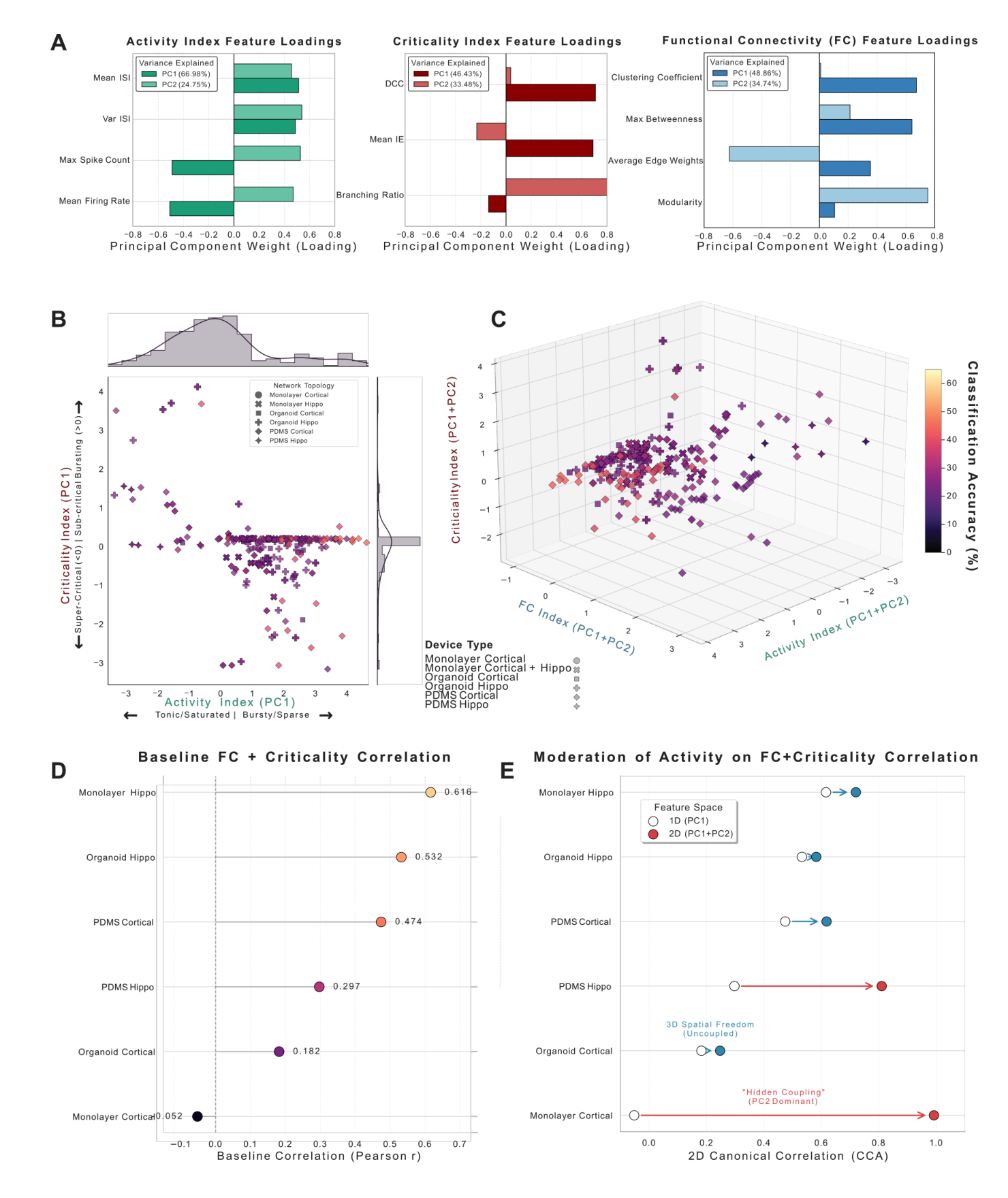
A Principal Component Analysis (PCA) feature loadings and explained variance (PC1 and PC2) for the Activity, Criticality, and Functional Connectivity (FC) indices. B 2D state-space of network Activity (PC1) versus Criticality (PC1) categorized by device type, featuring marginal distributions along both axes. C 3D composite landscape combining PC1 and PC2 for Activity, FC, and Criticality, with data points colored by Classification Accuracy (%). D Baseline 1D structure-function coupling (Pearson r ) across different device types. E Moderation of structure-function coupling, showing the Canonical Correlation Analysis (CCA) shift from a 1D (PC1) to a 2D (PC1+PC2) feature space, highlighting “Hidden Coupling” in 2D monolayers and spatial decoupling in 3D organoids.
Multi-Dimensional Structure-Function Coupling
Including a second topology component changes estimated structure-function coupling, especially in cortical monolayers. The authors interpret this as organization that a one-dimensional graph summary misses. Small, imbalanced groups and fitted multivariate correlations limit how strongly these results establish biological mechanisms.
Related references: [48].
3 Discussion
The main implication is that measured reservoir performance depends jointly on the living substrate, its physical organization, and the decoder. Reliable benchmarks must describe all three and establish the contribution beyond stimulation and analysis artifacts.
Cell type and architecture has a significant influence of electrophysiological network dynamics
Lineage and architecture produce distinct spontaneous dynamics. The authors propose studying how those dynamics change under structured feedback, rather than assuming that baseline criticality predicts learning during a task.
Related references: [51].
Cellular Composition and the Spatio-Temporal Reservoir
Cortical and hippocampal cultures differ in activity and temporal signatures. Their relative usefulness depends on structure and readout; combining lineages is a future direction, not a result established here.
Controlling Cell Culture Structures Highlights the Potential of Enforced Modularity
Microfluidic modularity may preserve separable responses by limiting global synchronization and constraining propagation. Modular cortical cultures lead the reported comparisons, but the explanation remains inferential. Once artifacts and split choice are controlled, digit accuracy is above chance and substantially below the largest headline values from permissive pipelines.
Related references: [5], [53], [54], [7], [21], [55], [26], [56], [57], [58], [59], [25], [60], [61].
Rigorous Controls Are Necessary to Mitigate Inflated Accuracies
Two failure modes dominate: direct decoding of electrical artifacts and spurious separation in high-dimensional feature spaces. Valid evaluation needs both appropriate sample splitting and controls that expose hardware, encoding, and readout contributions.
Decoding Methodology: The Unseen Variable
Frequency and spike-count representations capture different aspects of the same signals. Trial holdout estimates transfer to unseen trials; temporal holdout emphasizes persistence within a response. Decoder selection and the scientific prediction target must therefore be reported together.
Limitations and Future Directions
The study tests one task, two neural lineages, and uneven culture groups. It summarizes responses to repeated stimulus presentations and does not train cultures using closed-loop feedback. Performance of a learned external readout should not be interpreted as evidence of single-trial biological learning, general intelligence, or a demonstrated energy advantage over silicon.
4 Conclusion
Engineered modularity and careful frequency-domain readout are promising under this experimental protocol. Broader claims require balanced replication, additional tasks and cell mixtures, better three-dimensional recording, and feedback experiments measuring whether the cultures themselves improve.
5 Methods
5.1 Morphology and Organization of Neural Cell Cultures
Cultures are compared across monolayer, modular-film, and organoid configurations on microelectrode arrays. Baseline activity, evoked responses, lineage markers, and morphology characterize each preparation.
Related references: [69].
5.2 Differentiation of iPSCs to Cortical and Hippocampal Neurons
Differentiation protocols generate cortical and hippocampal neural populations from human induced pluripotent stem cells. The following sections retain the main preparation and selection distinctions.
5.2.1 Data Selection Criteria
Recordings are retained only when cultures pass the authors’ activity and data-quality criteria. Different architectures contact planar electrodes differently, which constrains the comparison.
5.2.2 Monolayer
Monolayers place differentiated cells on coated planar arrays, allowing relatively unconstrained network growth. Cortical and hippocampal preparations follow their respective maturation protocols.
5.2.3 PDMS Film 60-module Device
The PDMS film contains 60 connected modules, with microchannels permitting connections between neighboring wells. Cells mature within this imposed geometry before electrophysiological recording.
5.2.4 Organoid
Organoids are generated and matured as three-dimensional aggregates, then interfaced with the arrays. Planar electrodes sample only part of the volume; weak readout can reflect that interface as well as intrinsic computation.
5.3 Stimulation and Spike Sorting
The CL1 system delivers patterned stimulation and records extracellular voltage. Blanking and spike sorting reduce stimulation contamination before computing biological-response features.
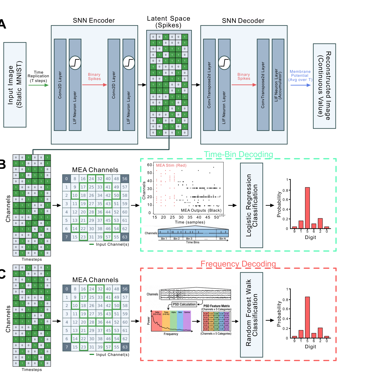
A: A static MNIST image is converted to a spatiotemporal spiking signal using a spiking autoencoder. The static MNIST image is flattened and replicated T times to convert it into a temporal signal. The resulting tensor is reduced into a smaller spatio-temporal signal of N by t via the autoencoding process. In this example N = 16 and t = 5. After training the autoencoder, the spatio-temporal latent signal is extracted and fed in as input to 16 channels of the MEA over 5 steps, delivered as a series of biphasic stimulation pulses. The resulting neural response was then decoded using each of the four mechanisms described in Decoding Mechanism 3 & 4: Time-Binned Spike-Count Decoding, Trial Holdout vs. Time Holdout (B) and Decoding Mechanism 1 & 2: Frequency-Domain (PSD) Decoding, Excluding vs. Including the Stimulation Window (C).
5.4 Classification
A trained artificial encoder generates the input patterns; separately trained readouts classify the culture responses. Neither training step constitutes supervised learning inside the living culture.
Conversion of Static Image to Spatio-temporal Spike-train
A spiking convolutional autoencoder maps each 28-by-28 MNIST image to a compact spatiotemporal spike pattern. Reconstruction training precedes the biological experiment. Latent spikes become biphasic electrical pulses on selected array channels.
Decoding Mechanism 1 & 2: Frequency-Domain (PSD) Decoding, Excluding vs. Including the Stimulation Window
Power spectral density in five frequency bands represents each response window. Random Forest classification uses cross-validation across trials; the comparison changes whether that window includes the stimulation period.
Decoding Mechanism 3 & 4: Time-Binned Spike-Count Decoding, Trial Holdout vs. Time Holdout
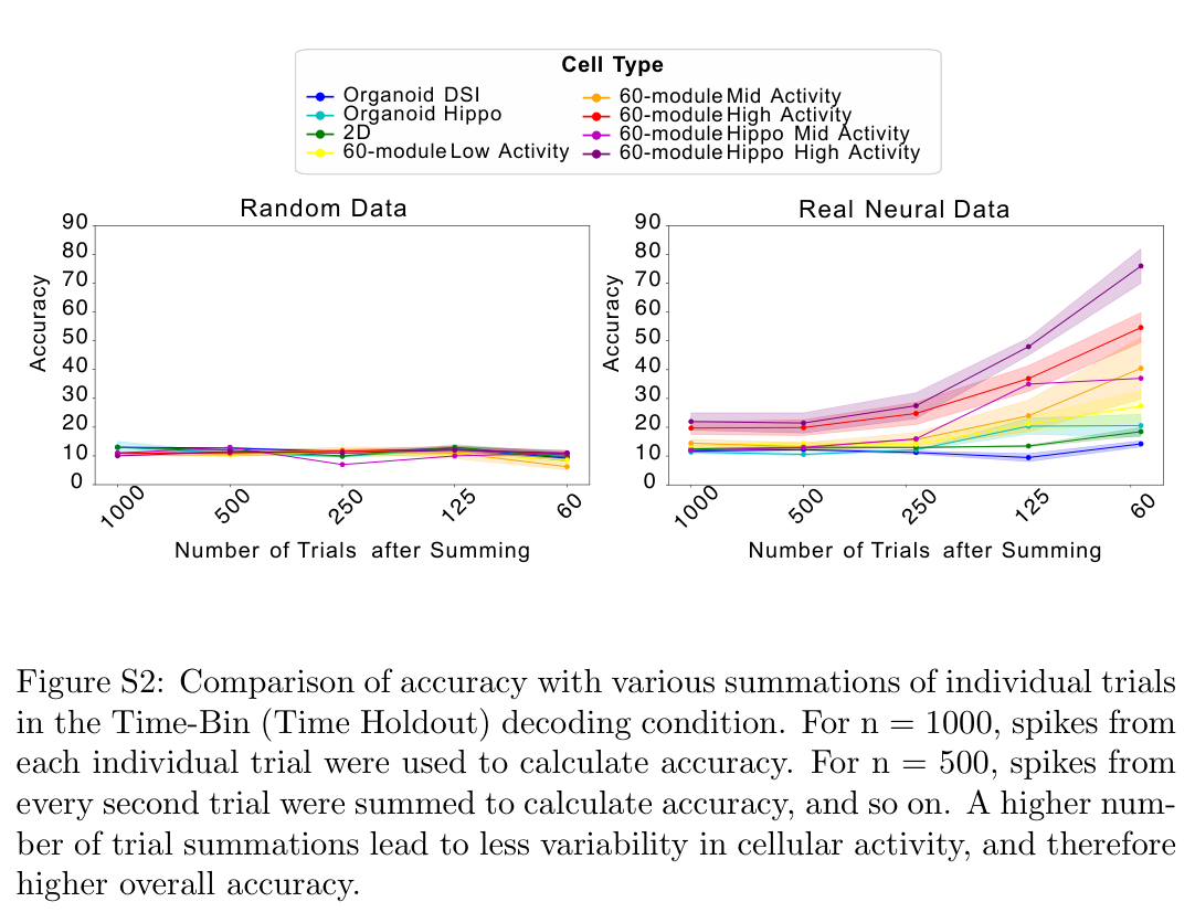
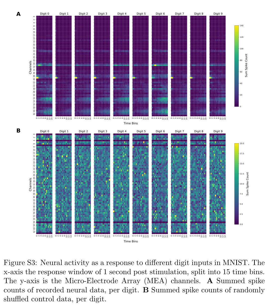
Spike counts are grouped into 66.7-millisecond bins and decoded with regularized logistic regression. Trial holdout separates recordings of stimulus presentations; time holdout separates bins from temporal response patterns.
Average Probability Decoding
Averaging predicted probabilities across repeated presentations can reduce response variability and improve digit discrimination. Such aggregation must be distinguished from the single-trial values preserved in Supplementary Table S5.
5.4.1 Controls
Controls include shuffled labels, randomized or synthetic spike responses, saline-only stimulation, direct decoding of the stimulation template, and a recurrent spiking-network simulation. Each targets a different source of apparently successful decoding.
5.4.2 Activity, Criticality and Functional Connectivity Metrics
Activity and avalanche measures describe firing dynamics; thresholded correlations define functional graphs. Statistical comparisons and dimensionality reduction relate these summaries to readout accuracy, with multiple-comparison corrections where specified.
Declarations
The full-text declarations identify Cortical Labs employment, share ownership, and related commercial interests. These disclosures are relevant to interpreting the platform evaluation.
Acknowledgments
The authors acknowledge Australian government support and collaborating institutions. Full funding and contributor details remain in the original preprint.
Supplementary tables and control figures
The supplement retains all six result tables and six control figures. It separates stimulus-blanked and stimulus-including frequency decoding, trial and time holdout, single-trial frequency decoding, and parameter sweeps on randomized data. Averaging repeated trials can improve separability; increasing feature dimensionality can also make randomized controls appear accurate. These comparisons are essential for interpreting the reported neural results.