At a glance
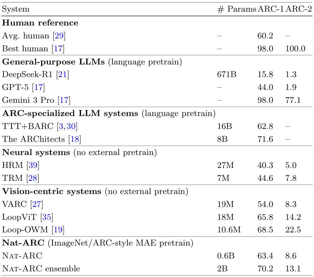
Nat-ARC asks whether representations learned from photographs help solve abstract grid puzzles. It initializes a vision encoder with ImageNet MAE weights, trains on ARC examples, then adapts separately to each unseen task. Matched comparisons across three model sizes find consistent gains over random initialization: the best ImageNet-pretrained single model reaches 63.4 ± 0.7% ARC-1 pass@2. Combining predictions from ImageNet-pretrained, ARC-grid-pretrained, and scratch models reaches 70.2 ± 0.6%.
The contribution is controlled evidence for visual pretraining transfer, rather than a new general-purpose reasoning system. ARC-2 remains substantially harder: the corresponding single-model and ensemble scores are 8.6 ± 0.8% and 13.1 ± 0.7%.
1. Why pretrain for abstract reasoning?
ARC presents small colored grids and a handful of input–output demonstrations; the solver must discover a transformation and produce an exactly correct new grid. Common rules involve shape, symmetry, filling, copying, or object relationships. Language-based solvers already inherit extensive pretraining, whereas many visual solvers learn largely from ARC supervision. Nat-ARC tests whether natural-image pretraining closes part of that asymmetry. [10] [12] [27]

3.1 ARC task and evaluation
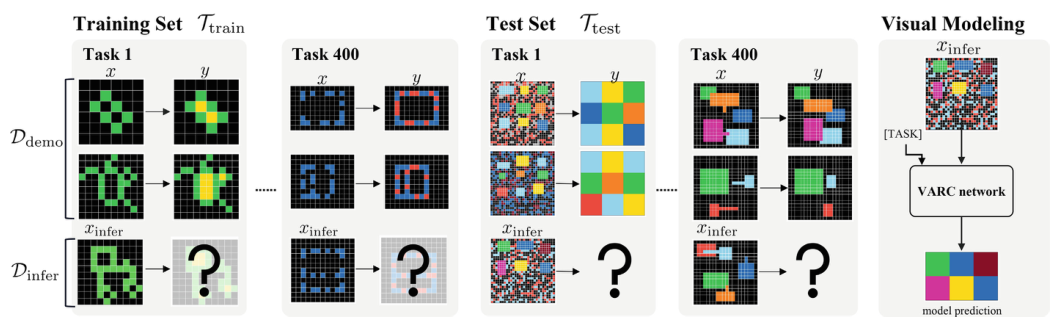
Each task provides a few demonstrations of a hidden mapping between grids, usually at most 30 × 30 cells with ten colors. A solver receives the new input but never its answer during adaptation. Training tasks and held-out evaluation tasks are separate; success requires the complete output grid to match exactly. Pass@2 allows two proposed outputs, rather than measuring per-cell correctness. [27]
3.2 Task-conditioned visual prediction
VARC places each input on a fixed canvas and predicts the output conditioned on a learned task embedding. Offline training learns across known tasks; test-time training adapts to a new task using only its demonstrations. Grid-preserving translations, scaling, rotations, flips, and color permutations enlarge the effective training set. The original objective is retained below. [27]
Equation 1

4.1 Three training stages
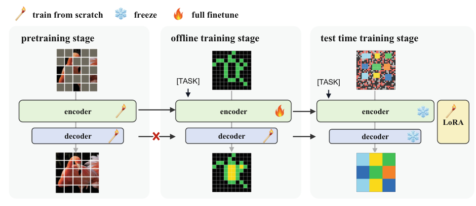
First, MAE learns an encoder by reconstructing masked image patches. Second, this encoder and a fresh decoder learn ARC mappings offline. Third, the resulting backbone is frozen while task-specific adapters and embeddings learn from each evaluation task. The study compares natural-image pretraining, ARC-grid pretraining, and no pretraining within the same downstream pipeline. [22] [16]
4.2 Encoder–decoder architecture
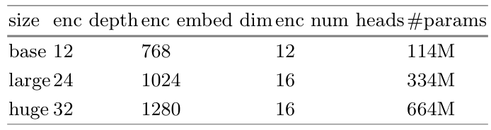
Each grid occupies a 64 × 64 canvas. Learned color embeddings are grouped into 2 × 2 patches, positional information is added, and a task token conditions the bidirectional Transformer. A lightweight decoder predicts color logits. All blocks use 2D RoPE. Only encoder capacity changes across experiments; total model sizes are 114M, 334M, and 664M parameters. [24]
4.3 Initialization, offline learning, and adaptation
ImageNet initialization. Public ImageNet-1K MAE weights initialize only the encoder backbone. Pretrained patch and absolute-position embeddings are discarded because ARC uses different input and patch sizes. The downstream model adds RoPE, absent from the public checkpoints; the supplement checks this mismatch. No additional ImageNet optimization is required. [22]
ARC-grid initialization. An alternative MAE is pretrained for 500 epochs with 75% masking on grids from 400 ARC-1 training tasks, about 400k RE-ARC pairs, and 1.5M NVARC pairs. Matching tokenization allows its encoder and embeddings to transfer. The decoder is initialized anew in all regimes. [25] [37]
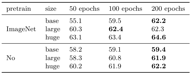
Offline and test-time learning. Every model trains for 200 epochs on ARC-1 demonstration pairs and RE-ARC. Inference pairs belonging to the training tasks are reserved for offline evaluation. At test time, each of the 400 unseen evaluation tasks gets independent adaptation using reversible augmentations. LoRA updates attention and MLP projections, while task embeddings are learned from scratch and the offline backbone remains frozen. [26]
4.4 Predictions and ensembles
Different translated, scaled, or rotated views yield candidate outputs, which are mapped back to the original grid. Candidates agree only when their entire grids match. The two most frequent distinct outputs provide pass@2 predictions. Ensembling pools candidates from different trained models and applies the same voting rule; it does not average weights or assume a shared latent representation.
5.1 Repeated-trial design
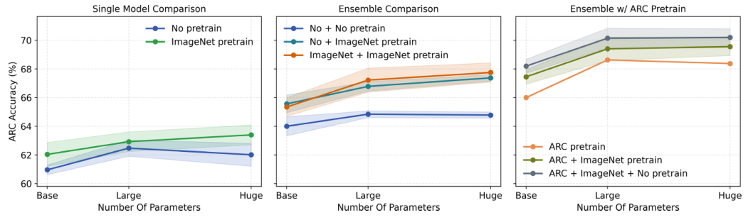
Each ImageNet-pretrained and scratch configuration uses five independent offline checkpoints. Two independent adaptation runs are averaged for each checkpoint, and the reported mean and standard deviation summarize the five resulting checkpoint scores. Ensemble statistics summarize combinations of checkpoints and their candidate predictions. Expensive ARC-grid pretraining uses only one offline checkpoint per size, so its single-model results have no checkpoint-level error bars.
5.2 Offline learning
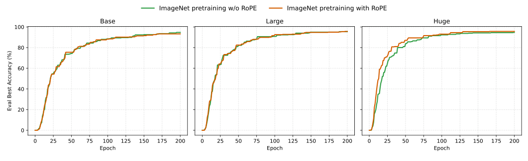
ImageNet initialization accelerates optimization at every tested scale and generally improves final offline accuracy. These curves evaluate held-back inference examples from the training-task set; they are not the final unseen-task benchmark. Each plotted trajectory represents one run.
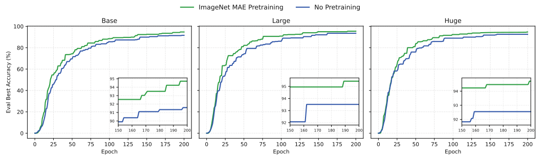
5.3–5.4 Unseen tasks and prediction ensembles
ImageNet pretraining improves final ARC-1 pass@2 over architecture-matched scratch baselines at every scale. Scratch performance rises from base to large but weakens slightly at huge size; pretrained models scale more consistently. Ensembles containing ImageNet-pretrained models outperform scratch-only ensembles. Two ImageNet models and mixed scratch/ImageNet pairs perform similarly.
ARC-grid pretraining is stronger in some comparisons but brings additional in-domain data and substantial pretraining cost. Combining all three initialization regimes gives the best ensemble result. The mixed ensemble therefore measures complementary visual solvers, while the matched single-model experiments provide the clearest evidence for natural-image transfer.
5.5 Comparisons and remaining gap
The system table provides context across human references, general language models, ARC-specialized language systems, and visual/neural approaches. Training data, parameter counts, access, and inference computation differ, so these scores are not controlled rankings. Nat-ARC still falls well short of the strongest reported systems, especially on ARC-2. Table values are the paper’s historical comparison, not a live leaderboard.
6.1 What attention visualizations show
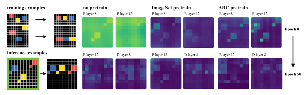
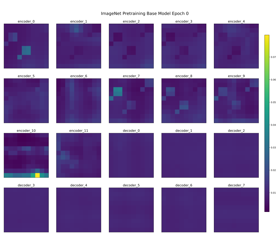
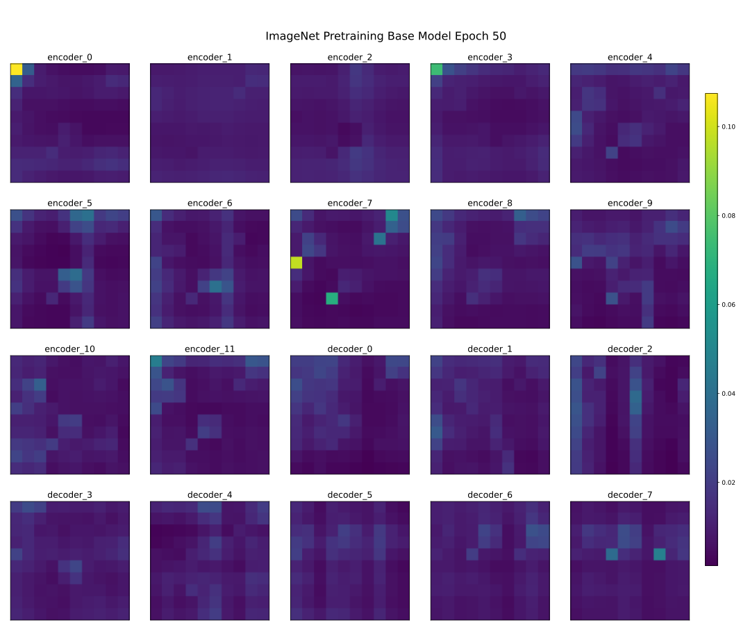
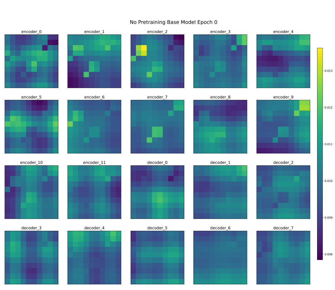
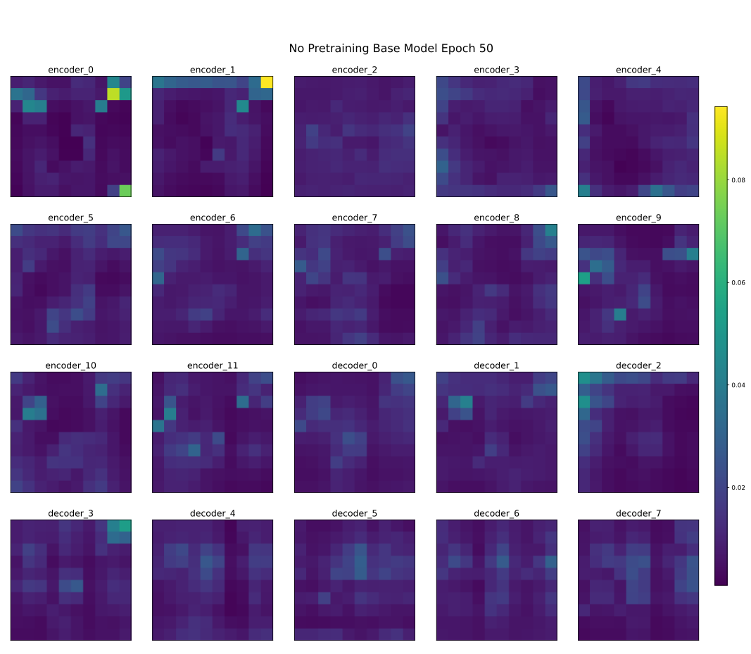
At initialization, MAE-pretrained encoders already emphasize foreground structure, including encoders pretrained solely on natural images. After 50 offline epochs, pretrained models show more output-related spatial organization than scratch models. These are descriptive attention patterns averaged over heads; they suggest a useful visual prior but do not establish a causal mechanism for reasoning.
6.2 Which tasks improve?
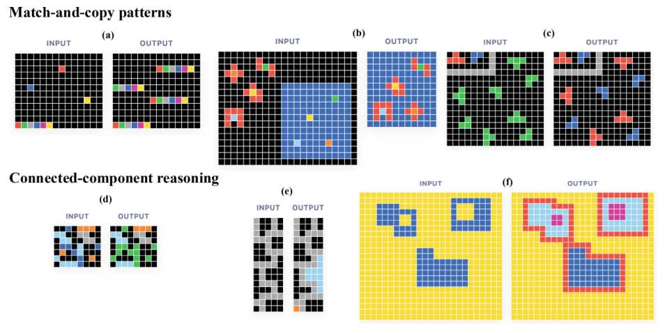
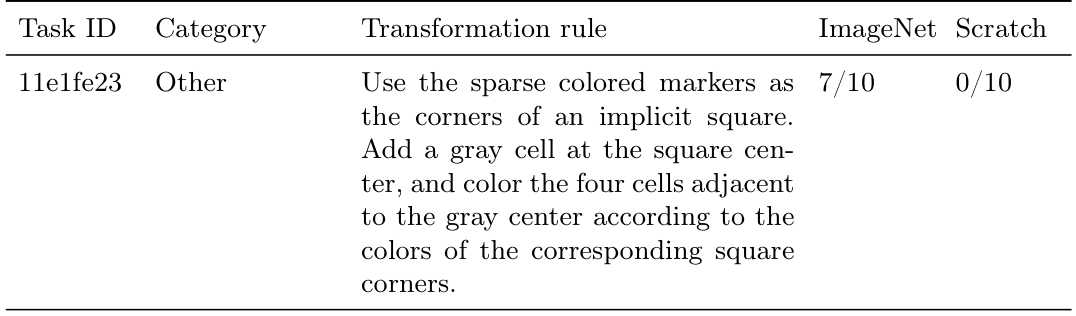
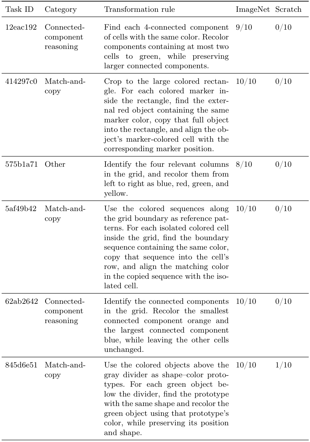
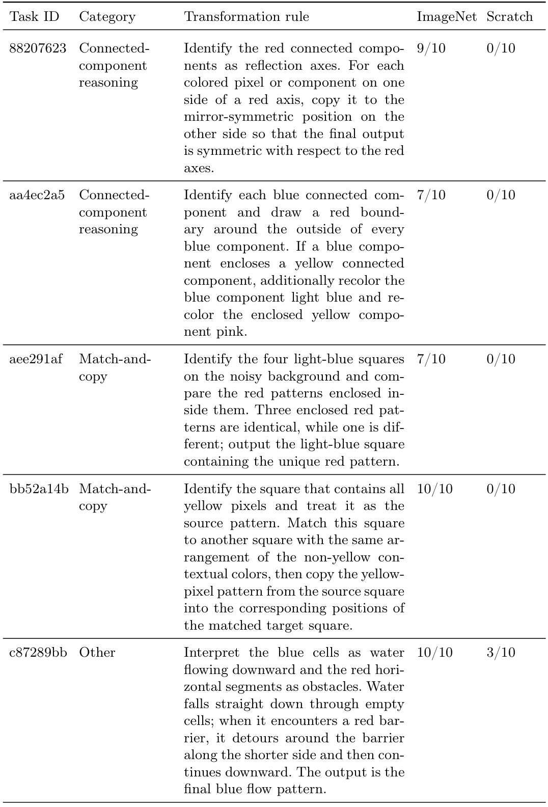
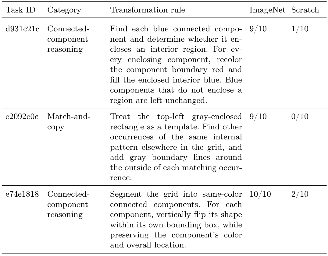
For huge models, all pairs of five checkpoints yield ten ensembles within each initialization family. The authors select tasks solved by at most 30% of scratch pairs and at least 70% of ImageNet pairs: fifteen tasks qualify. Manual inspection labels six as matching/copying, six as connected-component reasoning, and three as other transformations. This selected subset is evidence about recurring improvements, not an exhaustive taxonomy or an unbiased estimate of all ARC task types.
6.3 A toy bridge back to photographs
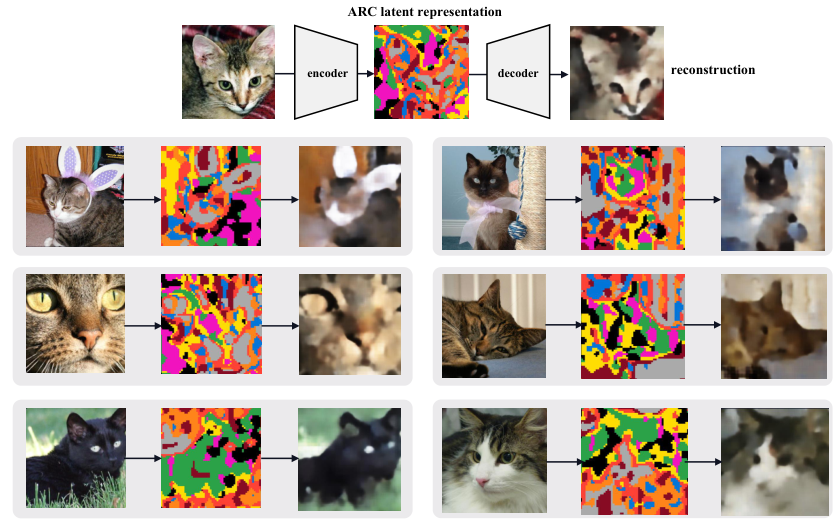
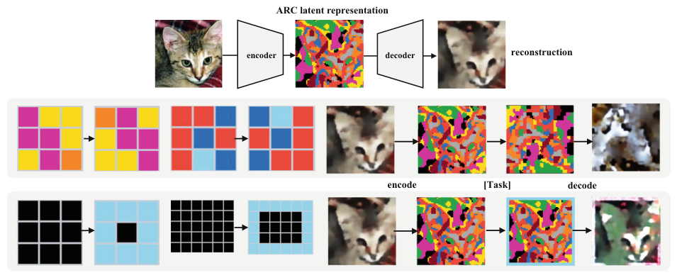
A separate autoencoder converts an ImageNet photograph into a 60 × 60 grid with ten possible symbols. This latent grid is placed on the ARC canvas, transformed by Nat-ARC under a chosen task token, then decoded into an image. A cat image is successfully rotated by 180° or given a border, despite some blur and quantization noise. The latent space was not explicitly aligned with ARC colors. These two qualitative examples demonstrate a possible connection between representations, rather than broad natural-image transformation performance.
7. Takeaway and limitations
Visual pretraining supplies representations that remain useful after supervised ARC learning and per-task adaptation. The strongest evidence is the repeated, matched comparison against random initialization. Larger models alone do not guarantee improvement; adaptation and voting remain important, ARC-grid results have fewer independent checkpoints, and ARC-2 scores expose substantial remaining difficulty. Attention maps and selected task examples suggest useful grouping and matching biases without fully explaining the mechanism.
Supplement A. Alternative pretraining
DINOv2 initialization improves its matched architecture from 53.6% to 60.7% ARC-1 pass@2. Architecture and adaptation differences prevent direct MAE comparisons.
Supplement B. Position encoding
Including RoPE during MAE pretraining changes offline performance little.
Supplement C. Adaptation ablations
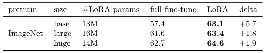
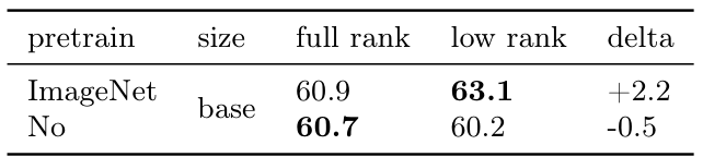
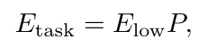
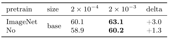
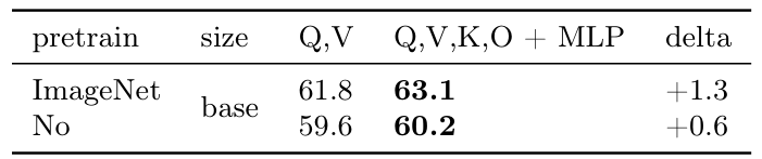
The ablations favor LoRA, rank-64 task embeddings, faster embedding updates, and adaptation of every linear layer. These recipe-selection runs differ from the repeated main results.
Equation S1, unnumbered
Supplement D. All fifteen selected tasks
The complete selected-task breakdown follows across four panels, retaining every transformation and solve count.
Supplement E. Offline training duration
Longer offline training generally improves accuracy.
Supplement F. Reproduction settings
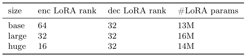
The retained settings specify each training stage. Adapter ranks vary by model size to maintain similar trainable parameter counts. [49]
- All stages use AdamW with linear warmup and cosine decay.
- Grid pretraining: 500 epochs, batch 1024, learning rate 0.001, weight decay 0.05, no dropout, 75% masking; a separate token marks input versus output grids.
- Offline learning: 200 epochs, batch 256, learning rate 0.0003, no weight decay, dropout 0.1.
- Adaptation: at most 100 epochs, batch 8, adapter learning rate 0.0002, task-embedding learning rate 0.002, embedding rank 64, weight decay 0.0003, LoRA dropout 0.1, and LoRA scaling equal to its rank.
- Every stage uses a 64-pixel canvas and 2-pixel patches. Adaptation stops after ten epochs without a training-loss improvement of at least 0.0001.
Supplement G. Full attention maps
All twenty layers are shown. Each figure uses an independent color scale; compare structure qualitatively.
Supplement H. Discrete image autoencoder
A Transformer encoder and Gumbel quantization produce ten-symbol grids; an upsampling decoder reconstructs images. The examples retain coarse content with visible blur.