At a glance
This edition covers Chapter 14, “Algorithmic statistics,” and both appendices of the 2017 book: printed pages 425–489, beginning at PDF page 434 in the circulated reading list. Chapter 14 asks when a short model explains an individual observation. The appendices connect complexity to statistical reasoning and compare four formal notions of randomness. Earlier chapters supply prerequisites; their full exposition is outside this excerpt. All four diagrams, displayed formula groups, three betting-history matrices, and the book’s complete bibliography are retained.
The central distinction is between describing data and explaining its structure. A good explanation is simple and makes the observed data typical. These are mathematical existence results based on generally uncomputable complexity, rather than an efficient recipe for learning a scientific theory.
14.1 Models and randomness deficiency
Represent an observation by a finite binary string x and a hypothesis by a finite set A containing it. The model must be specified completely, so its complexity C(A) includes knowing when the list ends. A desirable model has a short description, while x requires almost log₂|A| additional bits to identify within A. The difference, d(x|A) = log₂|A| − C(x|A), measures atypicality. Only a small fraction of a set can have large deficiency.
This deficiency is a universal effectively detectable test, up to additive constants. Prefix complexity gives an expectation-bounded variant. General finite rational distributions replace log₂|A| by −log₂P(x); restricting to uniform finite sets loses only controlled logarithmic precision. Allowing merely enumerable sets or lower-semicomputable probabilities would make explanations too permissive.
Equation Displayed formula 1 on printed page 426.

14.2 Stochastic and nonstochastic objects
A string is (α, β)-stochastic when some model costs at most α bits and leaves randomness deficiency at most β. Nonstochastic strings exist: some observations cannot be explained as typical outcomes of sufficiently simple models. The first counting argument gives 2α + β < n up to logarithmic terms; later results sharpen the boundary to α + β < n. Above the complementary boundary, every n-bit string has a suitable explanation.
Nonstochastic does not mean incompressible. Most strings are typical in the simple model containing every string of their length. The chapter bounds the fraction and universal prior mass of nonstochastic objects and relates stochastic finite prefixes to infinite random sequences under computable measures. One displayed inequality in the printed proof omits a minus before log P(x); the original image is retained, while the deficiency definition and subsequent inequalities use −log P(x).
Equations Displayed formula 1 on printed page 429.–Displayed formula 4 on printed page 430.





14.3 Two-part codes and statistical profiles
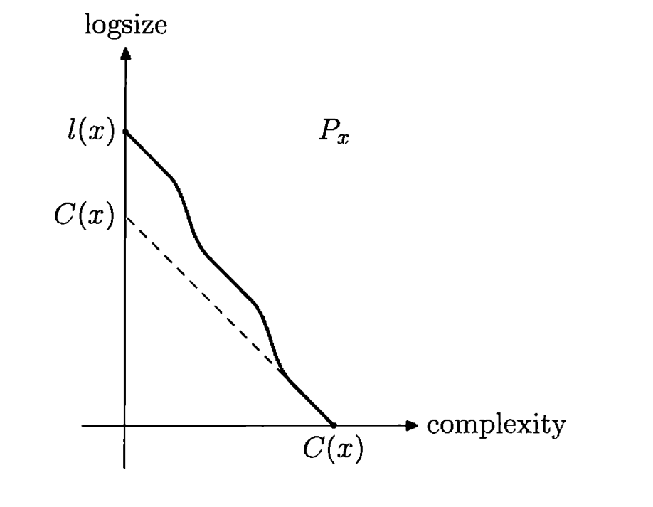
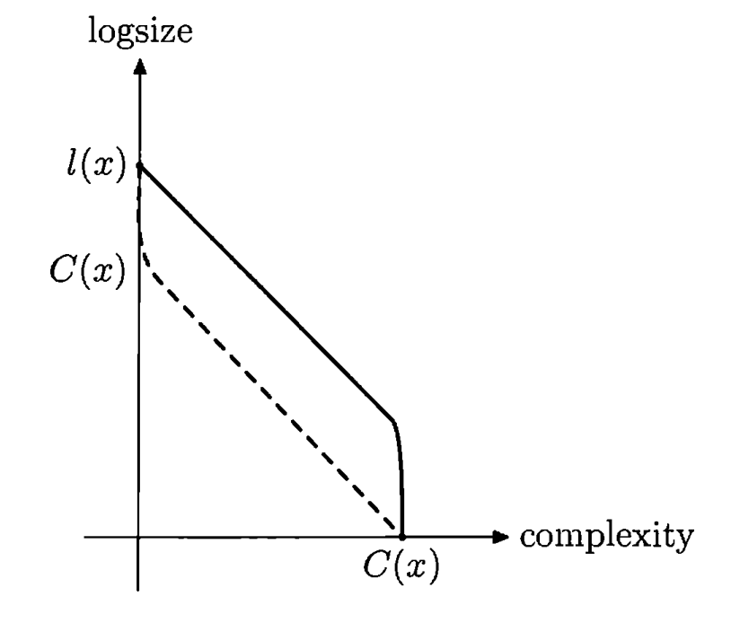
Describe the model, then the observation’s index inside it. The total length C(A) + log₂|A| upper-bounds C(x), with coding overhead. This motivates the Minimum Description Length (MDL) principle, but equal total lengths can allocate information differently. The profile Pₓ records achievable pairs of model complexity and log model size. It is upward closed; subdividing a model trades a smaller set for a longer model description.
The endpoints correspond to all n-bit strings and the singleton {x}. Between them, observations with the same length and complexity can have very different profiles. Essentially any suitably decreasing, simply described boundary can occur, allowing logarithmic error and the boundary’s description cost. The profile itself cannot be computed uniformly from x. Figures 52–53 show why a complexity number alone does not characterize explanatory structure. [60] [203]
14.3 Enumeration, multiplicity, and model information
Two-part descriptions have an equivalent interpretation in enumerations of all strings below a complexity threshold. Simple models place their members sufficiently early, or in suitably sized groups. Late appearance exposes a different kind of statistical structure from ordinary compressibility. Changing the threshold can change a string’s apparent unusualness.
If many distinct models describe the same observation, multiplicity can buy a shorter model or a smaller residual. An optimal boundary model is therefore simple given the observation; otherwise it carries avoidable information. A simple total computable bijection preserves the relevant profile properties, while small conditional complexities in both directions alone are insufficient.
Equations Displayed formula 1 on printed page 435.–Displayed formula 2 on printed page 435.


14.4 Restricting the model family
Practical explanations often come from a restricted family, such as Hamming balls describing bounded bit noise. The theory assumes an enumerable family containing every full set of strings of each length and satisfying an efficient covering property: smaller allowed sets cover larger ones with only polynomial overhead. Restricted profiles keep the endpoint and subdivision properties, but can be much worse than unrestricted profiles.
The exercises establish the covering property for Hamming balls and construct large gaps from unrestricted modeling. Under these assumptions, prescribed profile shapes remain realizable with approximately √(n log n) accuracy. The related lossy complexity Cᵣ(x) minimizes description length among strings within Hamming distance r. Uniform reconstruction from every permitted perturbation and reconstruction with a perturbation-dependent program are different requirements.
Equations Displayed formula 1 on printed page 439.–Displayed formula 1 on printed page 444.







14.4 Why many descriptions imply a better one
The selection theorem converts membership in many models into a simpler explanation. A two-player covering game proves that a limited collection of selected sets must cover every observation covered sufficiently often. Random selection gives an existence proof; an explicit greedy strategy repeatedly covers a substantial fraction of the remaining candidates. Its counting bounds yield the logarithmic description overhead.
Enumeration alone suffices for the multiplicity result that shortens the model. Reducing the residual size additionally uses the covering property. The construction is computable in the theoretical sense but has no practical runtime guarantee; neither this proof nor the shape-realization argument supplies an efficient general compression algorithm.
Equations Displayed formula 1 on printed page 446.–Displayed formula 2 on printed page 447.





14.5 Randomness deficiency versus optimality deficiency
Randomness deficiency asks whether x is typical inside A. Optimality deficiency δ(x|A) = C(A) + log₂|A| − C(x) asks whether the combined model-and-index code wastes bits. Randomness deficiency is bounded by optimality deficiency, up to logarithmic terms. Their gap is approximately C(A|x): information in the model that the observation does not justify.
A model can therefore make x typical while still being a poor explanation. However, replacing the model can remove that wasted information. The existence of a low-complexity model with small randomness deficiency is equivalent, at logarithmic precision, to the existence of one with small optimality deficiency. This transforms the two-part profile into a stochasticity profile and sharpens the nonstochasticity bounds. The statement compares achievable explanations, not the two deficiencies of every fixed model.
Equations Displayed formula 3 on printed page 447.–Displayed formula 4 on printed page 448.





14.6 Canonical minimal hypotheses
Enumerate all strings of complexity at most ℓ and let Nℓ be their total number. Split the enumeration into blocks whose sizes are the powers of two in Nℓ’s binary expansion. The block containing x is a canonical hypothesis. A block of size 2ˢ has model complexity approximately ℓ − s and lies near the statistical-profile boundary.
For any initial model A, choose ℓ as the maximum complexity of its members. The corresponding block B does not increase model complexity or optimality deficiency beyond logarithmic terms, and B is simple given A. Yet B’s information is essentially a prefix of the universal halting count, equivalently of a Chaitin Ω number. This cautions against identifying parameter-optimal models with meaningful scientific explanations. Total conditional complexity can distinguish models that ordinary complexity treats alike; other optimal models need not all share the same information. [199]
Equation Displayed formula 1 on printed page 450.

14.7 Interpretation: explanation and lossy compression
A theory can be viewed as a simple model of observations, with unexplained detail left in the residual index. Discarding that index suggests lossy compression or denoising: retain a clean recording plus a noise model, or a sand-dune shape plus a model of individual grains. Resampling a typical member preserves modeled structure without reproducing incidental noise.
This is an analogy about information, not a practical guarantee. Unlimited computation and uncomputable complexities are built into the framework, and canonical optimal models can encode halting information unrelated to the scientific story one hoped to discover.
Appendix 1: Probability, surprise, and evidence
Every particular long fair-coin sequence has the same tiny probability. Small probability alone therefore cannot explain why all zeros is suspicious while an irregular sequence is ordinary. The appendix separates two uses of probability: weighing possible consequences when applying an accepted model, and rejecting a model after observing an exceptionally unlikely, simply describable event.
The proposed complexity perspective refines the Cournot principle: surprising evidence is a simple low-probability event, not just an individually unlikely outcome. This is a discussion of foundations and practice, with explicit philosophical qualifications, rather than a new formal theorem. [180]
Appendix 1: Simple events, prior information, and frequencies
Requiring a suspicious event to be announced before an experiment avoids some post hoc selection, but an unexpectedly simple pattern can also be compelling. A bounded collection of simply described rare events still has small total probability. Conversely, repeating a previously observed complicated sequence is simple relative to that earlier information; conditional complexity captures why it can be suspicious.
Descriptions depend on the chosen language up to additive constants, and practical thresholds remain approximate. Defining probability solely through limiting frequencies does not remove the interpretive issue: finite experiments require saying that large deviations are unlikely. Frequency laws can instead be understood as consequences of excluding simple events of very small probability. Borel’s examples illustrate how attention to special numbers can distort surprise. [21] [22]
Appendix 1: Dynamics and the origin of random observations
Classical mechanics can connect a smooth distribution of initial conditions to outcome probabilities, as in dice throwing. That still leaves the distribution of initial conditions unexplained. The doubling map on the unit interval makes the issue precise: observing which half contains the state reveals successive binary digits of the starting point. Complexity in the observations was already present initially.
Deterministic computable evolution cannot create arbitrarily much descriptive complexity from a short initial state without supplying other information. This motivates a question about the physical source of apparently incompressible data, rather than proving that actual initial conditions possess any particular randomness property.
Equation Displayed formula 1 on printed page 460.

Appendix 1: Computationally limited observers
A pseudorandom generator expands a short seed into a long sequence with low unrestricted Kolmogorov complexity. Under standard computational hardness assumptions, efficient tests can nevertheless fail to distinguish its output from a truly random string. Knowing the seed immediately exposes its simple description; finding that seed may be computationally infeasible.
This separates mathematical incompressibility from operational unpredictability. Apparent randomness can reflect limits on an observer’s computation. The appendix raises this possibility for philosophical discussion without claiming that physical randomness is in fact generated this way. [61]
Appendix 1: A thermodynamic thought experiment
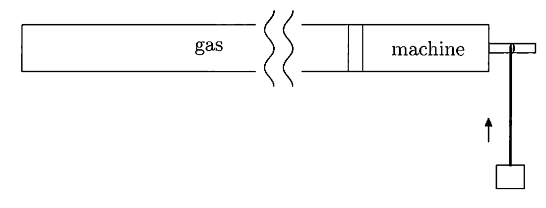
Consider a fixed-size machine that repeatedly extracts work from one gas reservoir. Under the stated assumptions, cooling a much larger gas system moves it toward a much smaller phase-space region. Measure-preserving dynamics cannot carry most initial states from a large region into that small destination. This sketches why a reliable perpetual-motion device of this kind is implausible.
The argument is deliberately informal: the initial-state distribution, interaction between subsystems, and precision of the machine’s preparation matter. It is not a general derivation of every formulation of the second law from time-reversible dynamics.
Appendix 1: Quantum probabilities
The final analogy replaces classical probabilities by quantum amplitudes. Events with very small amplitude receive little practical weight; for many independent systems, the amplitudes of large deviations in outcome frequencies are small. This links observed frequencies to squared amplitudes in the discussed product-system setting.
The passage is a conceptual comparison between interpreting probabilistic models and quantum models. It does not resolve the measurement problem or derive the full foundations of quantum theory.
Appendix 2: Four algorithmic faces of randomness
Uspensky’s essay begins with equally likely finite strings that evoke different intuitions about randomness. Distribution matters, short strings offer little basis for judgment, and finite randomness has no sharp intuitive cutoff. Infinite sequences permit precise definitions, although their connection to finite observations requires care.
The four candidates are stable frequencies under admissible selection, incompressibility, membership in all effective probability-one classes, and resistance to computable betting. The appendix uses “entropy” for description complexity and special names for these properties; its notation differs from the main chapters. Cylinder sets consist of sequences with a specified finite prefix and have fair-coin measure 2 to the negative prefix length.
Equations Displayed formula 1 on printed page 465.–Displayed formula 4 on printed page 465.




Appendix 2, face one: Frequency stability
Limiting frequency one-half is insufficient: an alternating sequence passes that test. Von Mises therefore required stability in admissibly selected subsequences. Church’s rule decides whether to keep the next bit using only earlier revealed bits. Kolmogorov–Loveland selection also chooses which unrevealed position to inspect, so selected positions need not preserve their original order.
Before revealing a bit, the algorithm chooses both its position and whether to retain it. Repeated positions or undefined choices stop the construction; only infinite retained subsequences must have the required limiting frequency. This stronger stochasticity class is still too broad: some such sequences have more zeros than ones in every prefix, unlike typical fair-coin random walks.
Equations Displayed formula 1 on printed page 468.–Displayed formula 4 on printed page 470.






Appendix 2, face two: Incompressibility
Description complexity is the length of the shortest binary description in a chosen computably enumerable description language. An optimal language simulates every competitor in the family with constant overhead, making the resulting complexity invariant up to an additive constant.
For infinite-sequence randomness, the choice of description family matters. Monotone descriptions require compatible inputs to produce compatible outputs. A sequence is “chaotic” when every length-n prefix has monotone complexity KM at least n minus a fixed constant. This is not the false requirement that every prefix have plain complexity n minus a constant. The use of monotone complexity supplies the correct infinite-sequence criterion.
Equations Displayed formula 1 on printed page 471.–Displayed formula 3 on printed page 475.












Appendix 2, face three: Effective typicality
Ordinary measure-zero sets are too broad: every individual infinite sequence belongs to one. Restrict attention to sets that can be covered effectively, uniformly in a requested error bound, by cylinders with arbitrarily small total measure. A Martin-Löf random sequence avoids every such effectively null set.
There is a universal effective test. The complement of its null set gives the smallest effective probability-one class. The Levin–Schnorr equivalence identifies this typicality class with the monotone-incompressibility class. It is a strict subclass of Kolmogorov–Loveland stochastic sequences, so stable selected frequencies alone do not characterize this notion of randomness.
Equations Displayed formula 4 on printed page 475.–Displayed formula 3 on printed page 476.




Appendix 2, face four: Computable betting
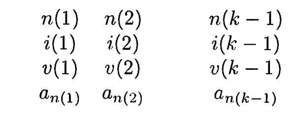
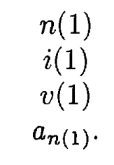
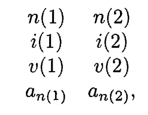
A player selects an unrevealed position, predicts its bit, and stakes a nonnegative rational amount smaller than current capital. Correct predictions add the stake and incorrect ones subtract it. A computable strategy may choose positions adaptively and may be partial; an undefined move leaves capital unchanged. Winning means unbounded capital, sufficient to exhaust any fixed casino bankroll.
The history matrices record positions, predictions, stakes, and revealed outcomes. For a fixed strategy, the revealed bits reconstruct the rest of the history. Martin-Löf randomness implies resistance to these nonmonotone computable betting strategies, which in turn implies Kolmogorov–Loveland stochasticity; the latter inclusion is strict. The book presents equivalence of the first two classes as an open question in its account. This edition reports that historical status rather than asserting an updated resolution.
Equations Displayed formula 1 on printed page 477.–Displayed formula 2 on printed page 478.






Equations Displayed formula 1 on printed page 479.–Displayed formula 2 on printed page 480.




Appendix 2: Arbitrary computable distributions
For a general measure, cylinder probabilities replace uniform bit counts. Bernoulli trials use one fixed bias; quasi-Bernoulli trials allow a different bias at each position. A computable measure provides rational approximations to cylinder probabilities to any requested accuracy. Deciding whether a cylinder has exactly zero measure is an additional requirement, and computing an exact rational value is stronger than approximating a value known to be rational.
The essay extends all four definitions to computable measures. The same implication structure holds; the strict separation between stochasticity and betting resistance is stated with positivity of all cylinders. Randomness is always relative to the proposed distribution, rather than a property independent of the model.
Equations Displayed formula 3 on printed page 480.–Displayed formula 4 on printed page 481.





Appendix 2: Selection under nonuniform measures
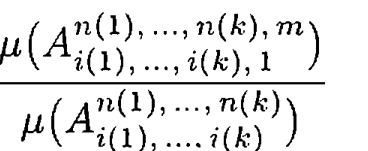
For independent biased bits, selected observed frequencies must track the average of their selected success probabilities. For dependent distributions, use each selected bit’s conditional probability given all previously revealed bits, including revealed bits that were not retained. The average difference between these probabilities and the selected outcomes must tend to zero.
This requirement applies to every admissible rule producing an infinite subsequence. Conditional probabilities must be defined; histories of zero measure require special handling. The formulas distinguish the intermediate revealed sequence from the final retained sequence, a distinction essential for adaptive selection.
Equations Displayed formula 1 on printed page 483.–Displayed formula 2 on printed page 484.









Appendix 2: Incompressibility and typicality under a measure
Replace the prefix length benchmark by its information content, −log₂ of the cylinder probability. A sequence is incompressible relative to a computable measure when monotone descriptions cannot substantially improve on that benchmark, uniformly over prefixes.
Effective typicality similarly uses covers with small total measure instead of small uniform volume. The universal effective test and the equivalence between typicality and incompressibility extend to these computable distributions. The essay calls the resulting smallest effective probability-one class the measure’s constructive support.
Equations Displayed formula 3 on printed page 484.–Displayed formula 1 on printed page 485.



Appendix 2: Fair odds and zero-probability outcomes
Unequal probabilities require unequal payouts. A correct prediction earns the stake multiplied by the conditional probability of the alternative outcome divided by that of the predicted outcome. A wrong prediction loses the stake. This maintains zero conditional expected gain.
If the revealed history first has measure zero, the additional stopping rule assigns infinite capital to a correct prediction and leaves capital fixed after an incorrect prediction. Strictly smaller-than-capital stakes support effective validity checking even when capital is a computable real. The rules preserve the intended betting notion while avoiding an undefined division by zero.
Equations Displayed formula 2 on printed page 485.–Displayed formula 2 on printed page 486.








Appendix 2: History, terminology, and further reading
The historical notes trace selection rules to von Mises, Church, and Kolmogorov–Loveland; descriptive complexity to Solomonoff, Kolmogorov, and Chaitin; effective tests to Martin-Löf; and the incompressibility connection to Levin and Schnorr. Monotone, prefix, process, and a priori complexities differ as functions but give the same prefix-incompressibility randomness class here. Plain and decision complexities do not.
Description complexity measures objects, while computational complexity measures resources used by computations. The appendix also explains why translations and differing uses of “entropy,” “stochastic,” and “random” can obscure comparisons. Its eight local references are included after the 225-entry book bibliography, labeled “Appendix 2” to keep the two numberings distinct. [Appendix 2, 1] [Appendix 2, 3] [Appendix 2, 5] [Appendix 2, 8]
Equations Displayed formula 1 on printed page 488.–Displayed formula 1 on printed page 489.

