At a glance
A large convolutional network trained on labeled ImageNet images substantially improves object recognition. Five convolutional layers and three fully connected layers combine ReLU activation, two-accelerator training, data augmentation, and dropout. The 2012 winning result is a seven-model ensemble, partly pretrained on more ImageNet categories: 15.3% top-five test error versus 26.2% for the runner-up.
1 Introduction
Large image datasets make high-capacity supervised models practical, while convolution supplies useful assumptions about local structure and shared visual patterns. Efficient accelerator implementation makes training feasible. The paper’s achievement combines architecture, compute, and regularization; no single ingredient alone explains the result.
2 The dataset
The competition subset has about 1.2 million training images, 50,000 validation images, and 150,000 test images across 1,000 categories. Images are resized and center-cropped to 256 × 256, then mean-centered. Top-one error checks the highest-ranked class; top-five error checks whether the correct class appears anywhere among five predictions.
3 The architecture
The network has eight learned layers, approximately 60 million parameters, and 650,000 neurons. The following components improve training speed or generalization within this specific design.
3.1 ReLU nonlinearity
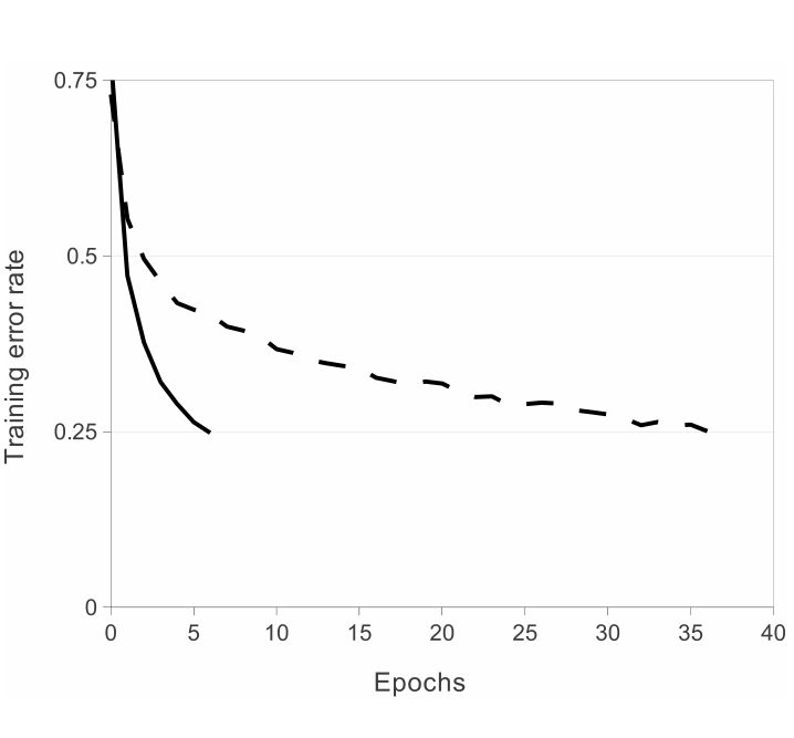
Rectified linear units use the positive part of their input and avoid saturation on that branch. In a four-layer CIFAR-10 comparison, they reach 25% training error about six times faster than tanh. Faster optimization enables practical experiments with the much larger model. See the earlier rectified-unit work in [20].
3.2 Training on multiple accelerators
The model is split across two accelerators because one has only three gigabytes of memory. Most groups communicate locally, with cross-device connections in selected layers. The larger two-device architecture improves accuracy while controlling communication cost; the comparison is not a pure test of parallel execution at fixed architecture.
3.3 Local response normalization
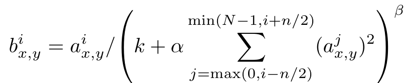
Local response normalization divides each activation by a term depending on nearby channel activations at the same spatial location. It encourages competition between large responses and improves this model’s reported errors. The hyperparameters are selected on validation data; the preserved equation specifies the operation.
Equation Local response normalization
3.4 Overlapping pooling
Overlapping max pooling uses 3 × 3 windows at stride two. Compared with nonoverlapping pooling of equal output dimensions, it slightly improves top-one and top-five error and appears to reduce overfitting.
3.5 Overall architecture
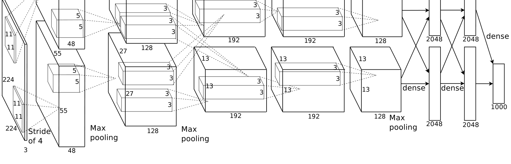
The convolutional widths are 96, 256, 384, 384, and 256 filters, followed by two 4,096-unit hidden layers and a 1,000-way softmax. ReLU follows learned hidden layers. Normalization follows the first two convolutions, and pooling follows those normalized outputs and the fifth convolution. The original architecture figure preserves spatial sizes and the two-device connectivity.
4 Reducing overfitting
Even 1.2 million labeled images do not eliminate overfitting in a 60-million-parameter model. Image augmentation and dropout are the main countermeasures.
4.1 Data augmentation
Training samples random 224 × 224 crops and horizontal reflections. Evaluation averages ten crop predictions. Color augmentation adds randomly scaled principal components of training-set color variation, with one perturbation shared across each image. These transformations preserve labels while exposing variation cheaply during training.
Equation Principal-component color perturbation

4.2 Dropout
Dropout independently suppresses half the hidden activations in the first two fully connected layers during training. At evaluation all units are used with scaled outputs. It reduces co-adaptation and substantial overfitting, at roughly twice the iterations needed to converge. The technique is introduced in [10].
5 Details of learning
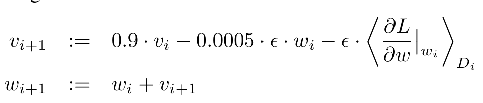
Training uses SGD with batch size 128, momentum 0.9, and weight decay 0.0005. Weights begin as small Gaussian samples; selected biases start at one to activate rectified units. The learning rate begins at 0.01 and is manually reduced when validation error stops improving. About 90 epochs take five to six days on two contemporary accelerators.
Equation Momentum and weight-decay update
6 Results
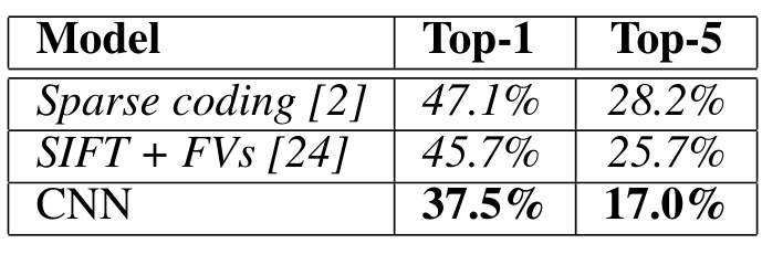
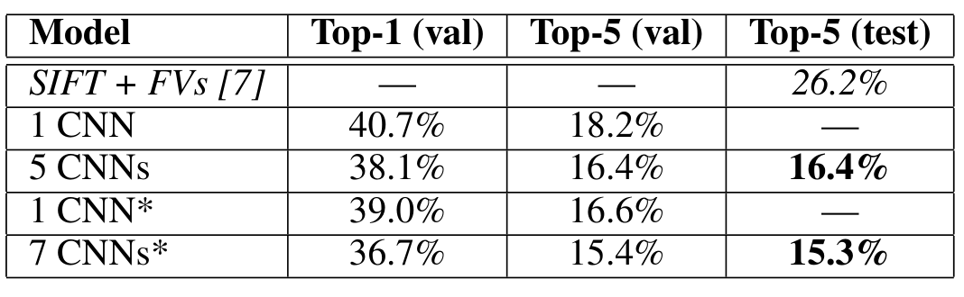
On ImageNet 2010, the network achieves 37.5% top-one and 17.0% top-five test error with crop averaging. For 2012, one model has 18.2% top-five validation error; five-model averaging reaches 16.4%. Combining these with two models pretrained on the larger 2011 ImageNet release gives the winning 15.3% test error. The tables preserve the distinctions between single models, ensembles, pretraining, validation, and test.
6.1 Qualitative evaluations
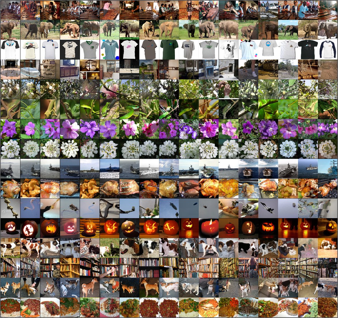
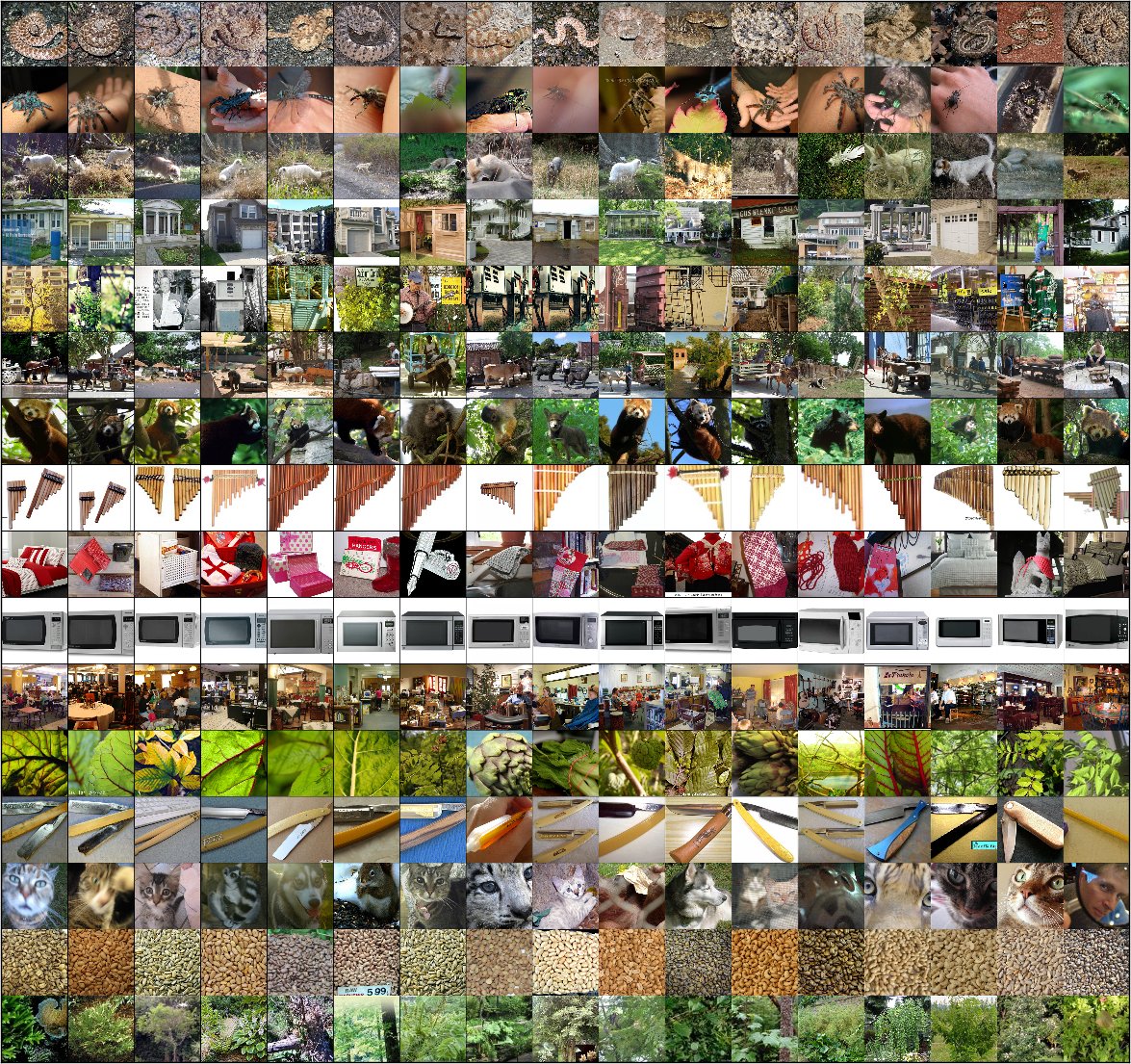
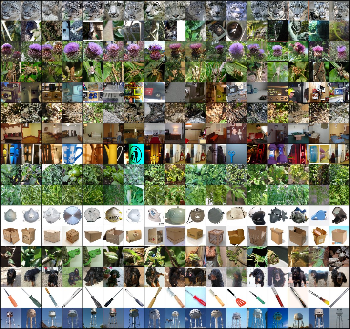
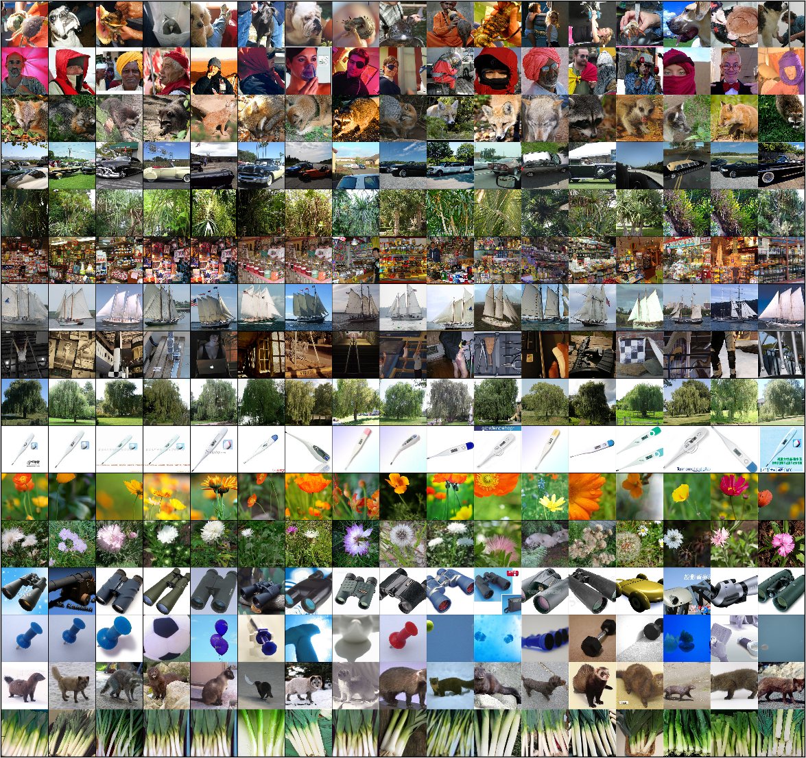
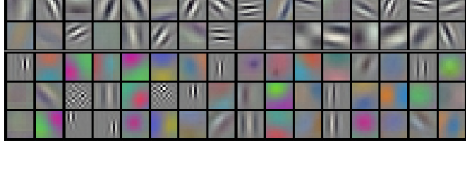
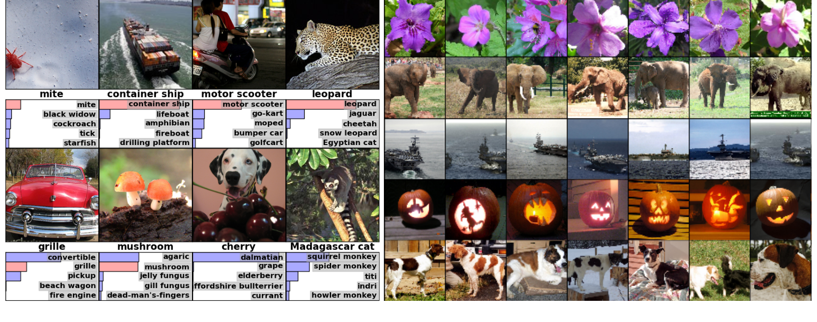
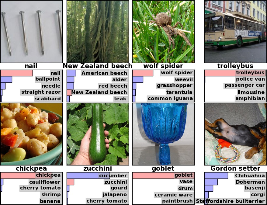
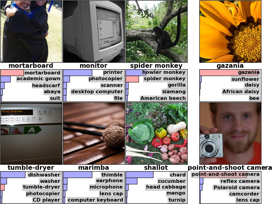
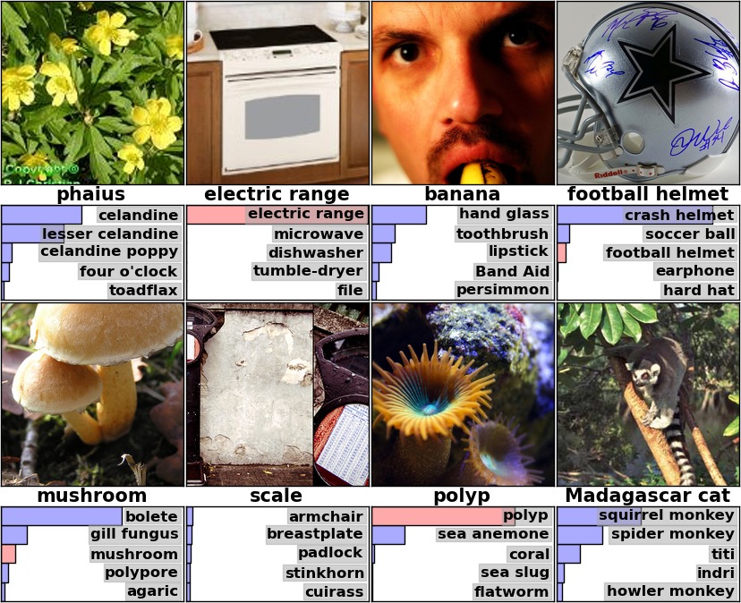
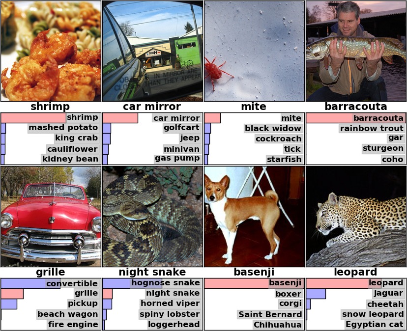
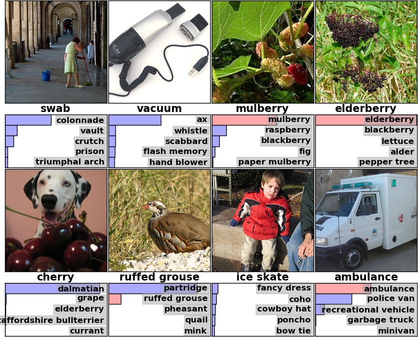
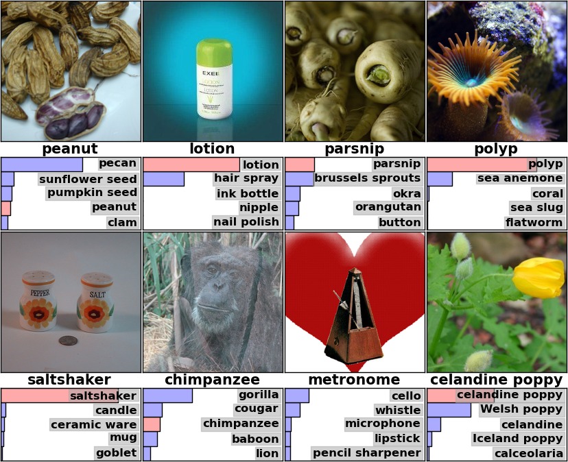
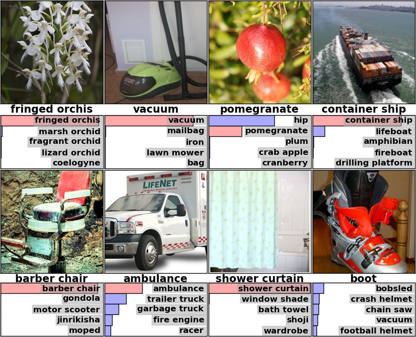
First-layer filters learn oriented patterns and color-sensitive features, with different specializations across the two device groups. Nearest neighbors in the last hidden layer share semantic content despite different pixel layouts. Prediction examples also reveal ambiguity about which object a photograph is intended to label; these illustrations are qualitative, not a separate robustness benchmark.
7 Discussion
Removing any convolutional layer hurts performance, supporting the importance of depth within this architecture. The work shows that supervised learning at sufficient scale can strongly outperform the contemporary alternatives. Larger models, more data, and video are proposed directions; the experiment does not establish unrestricted generalization beyond ImageNet.
Supplement: learned feature maps
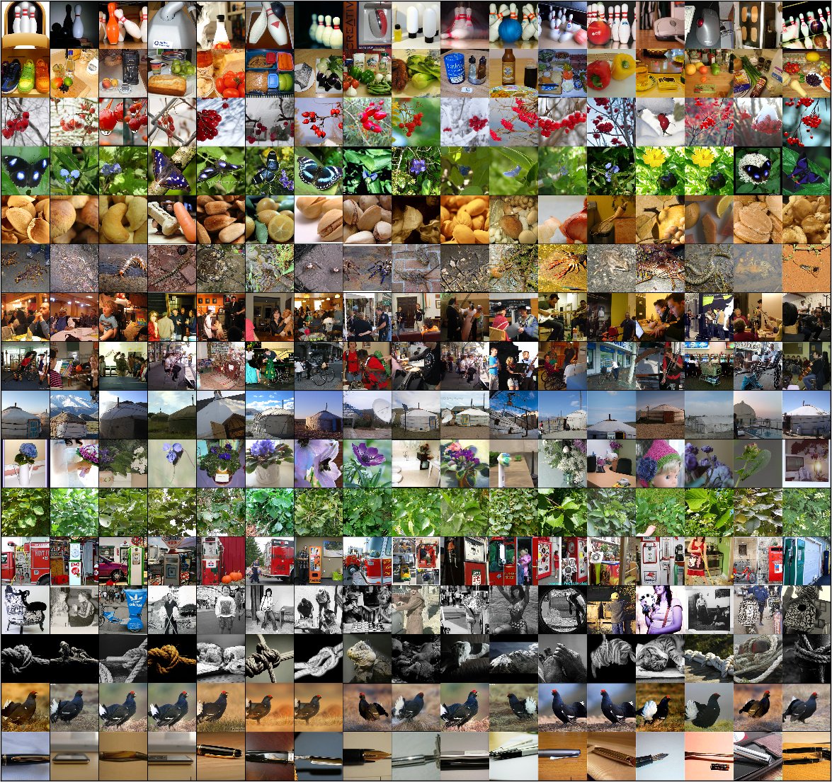
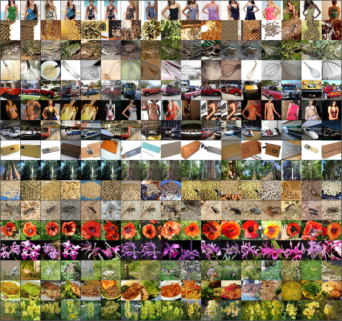
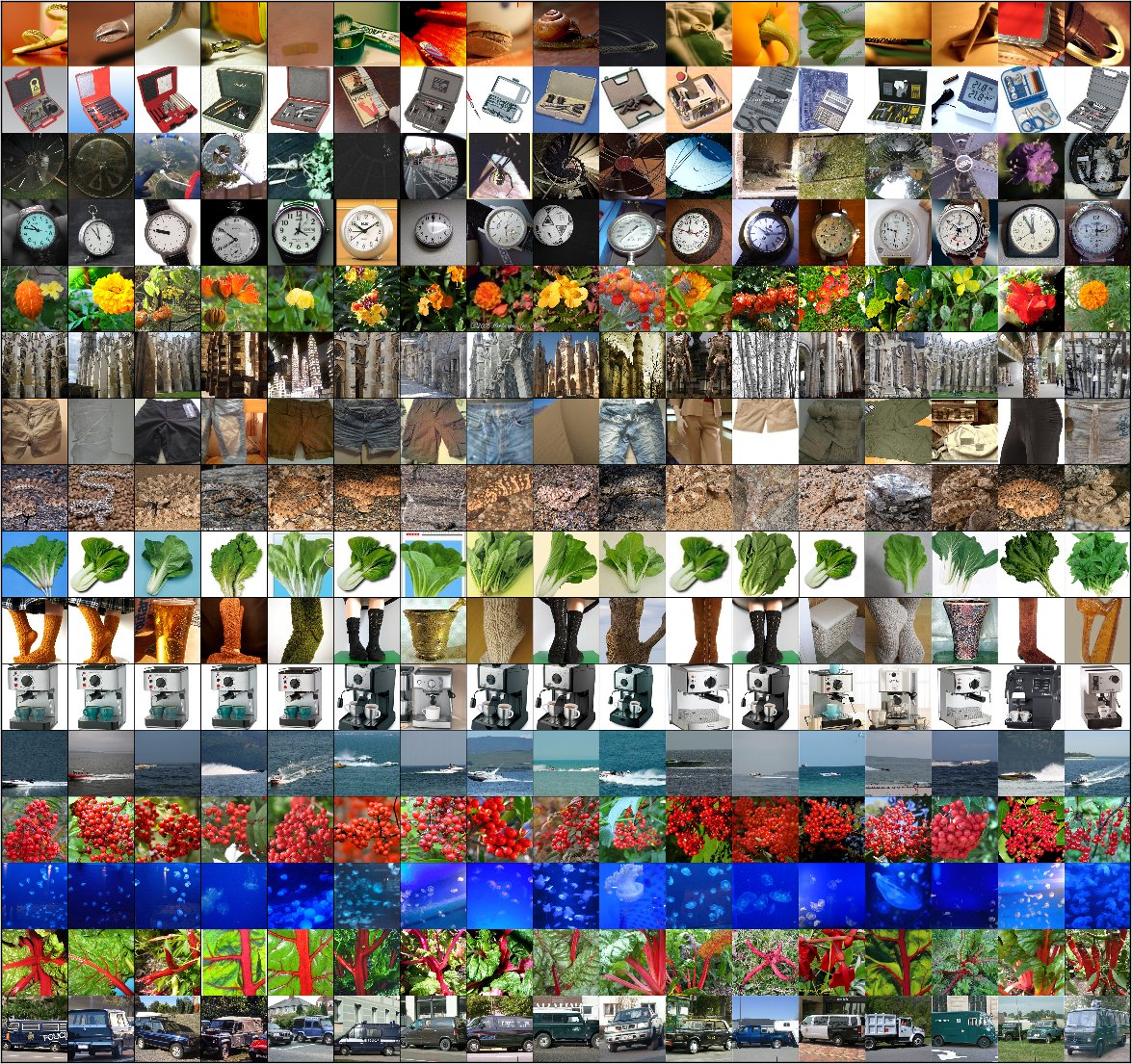
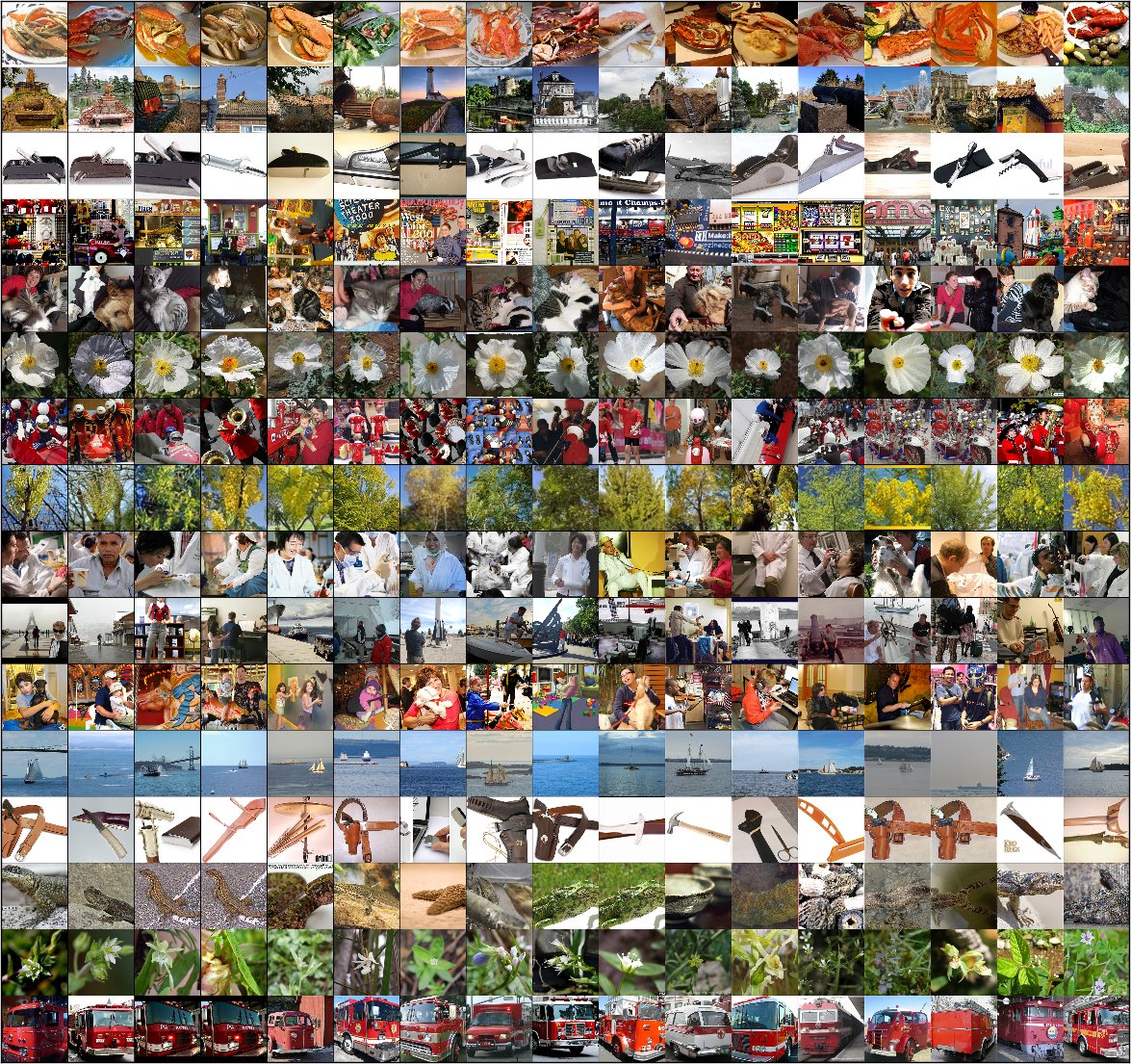
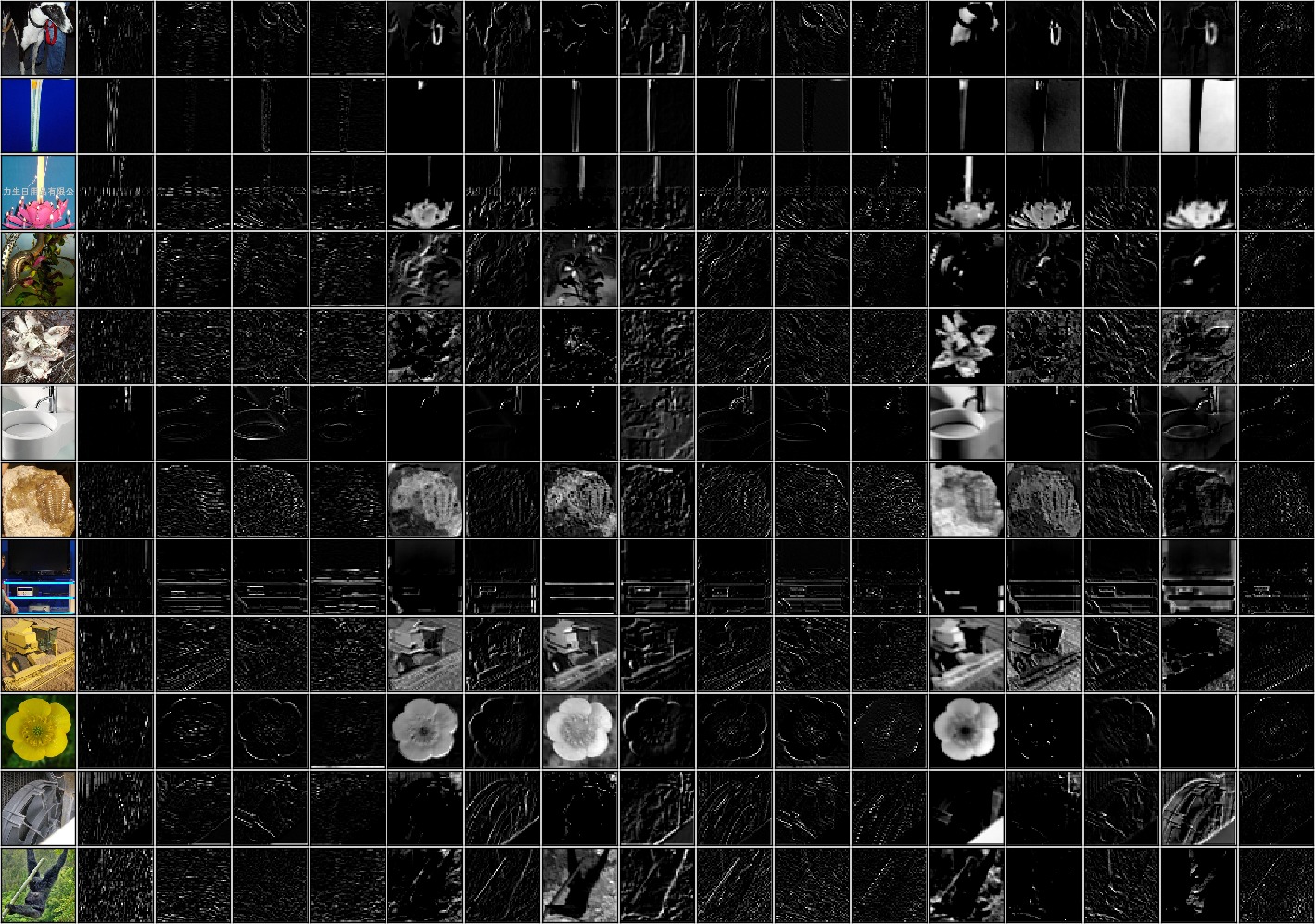
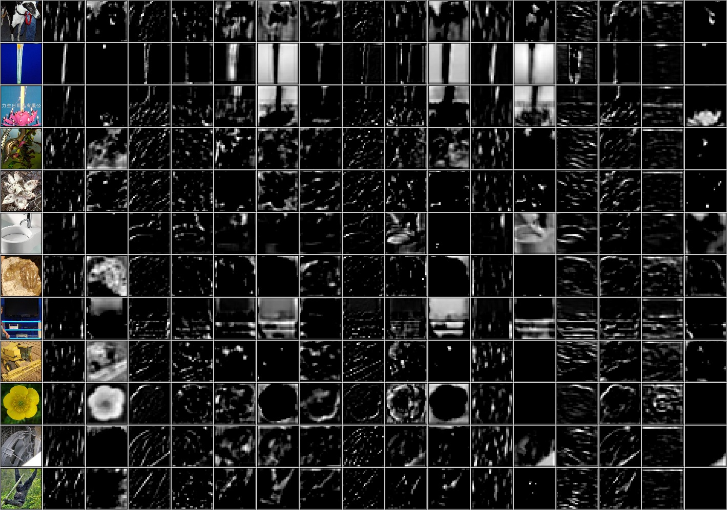
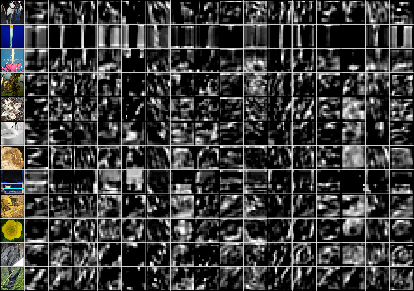
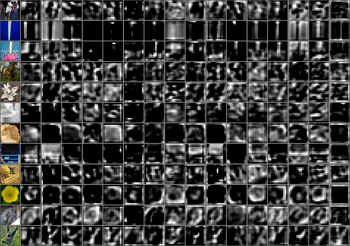
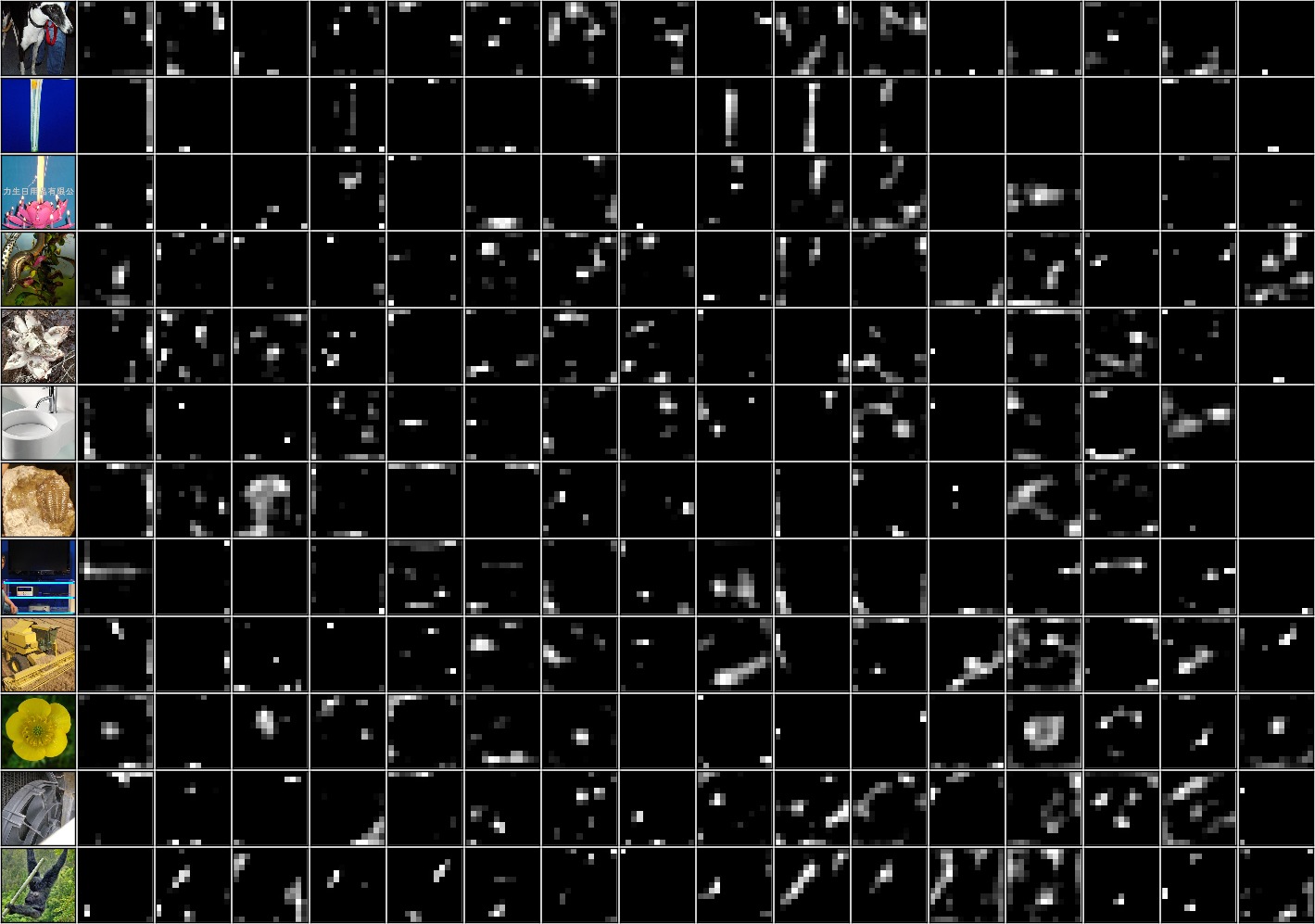
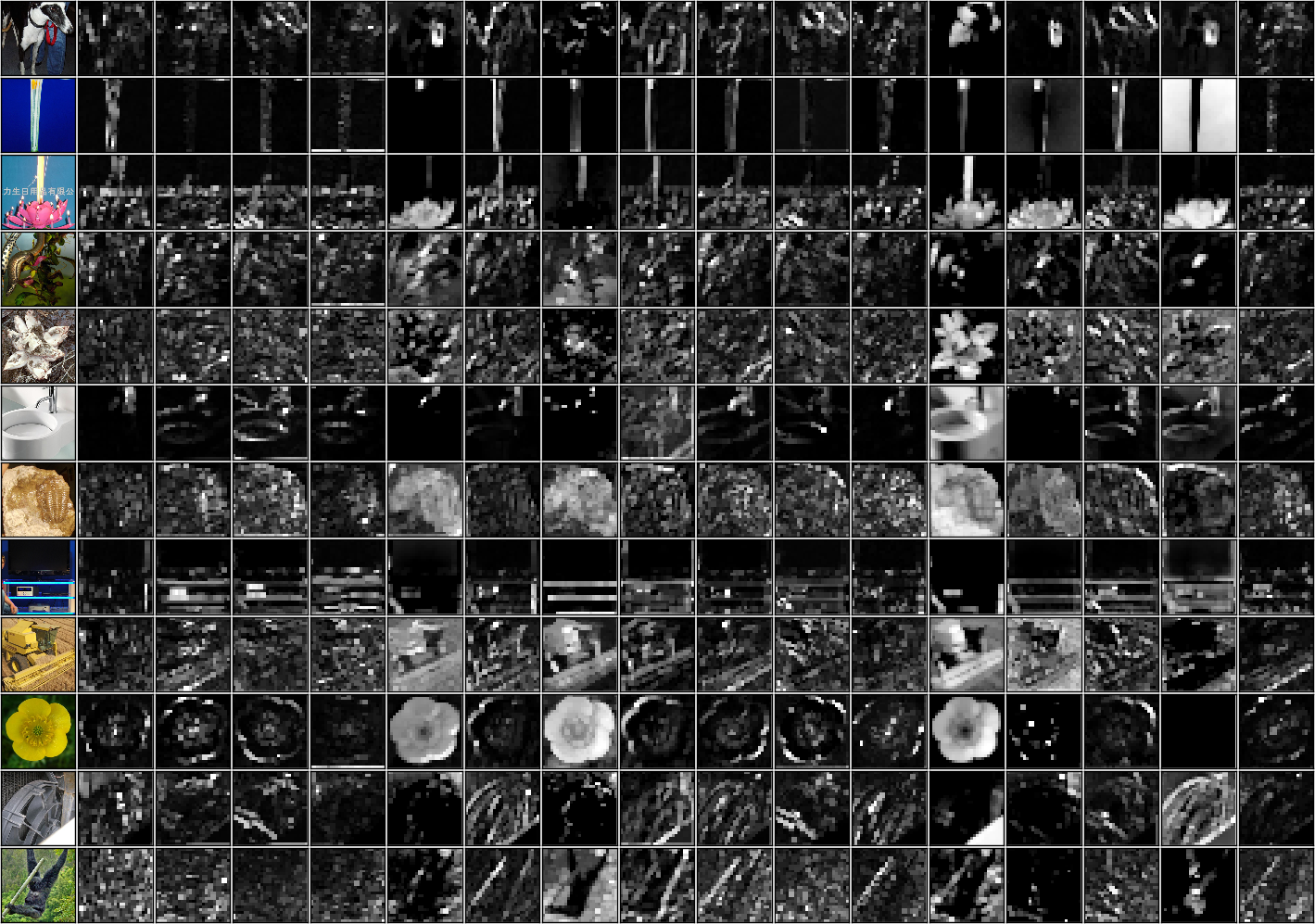
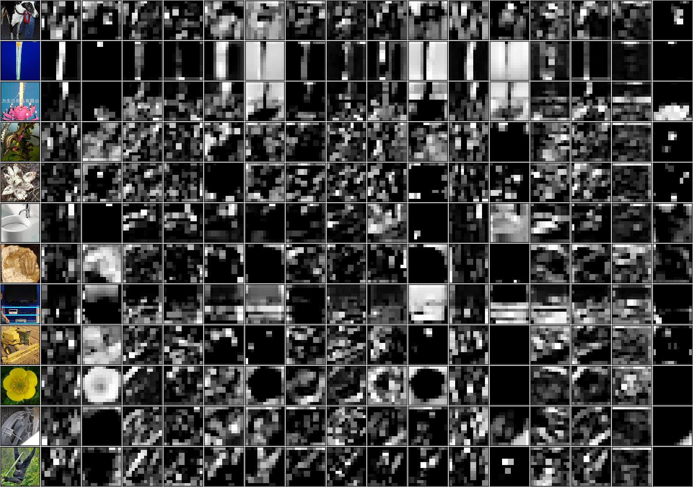
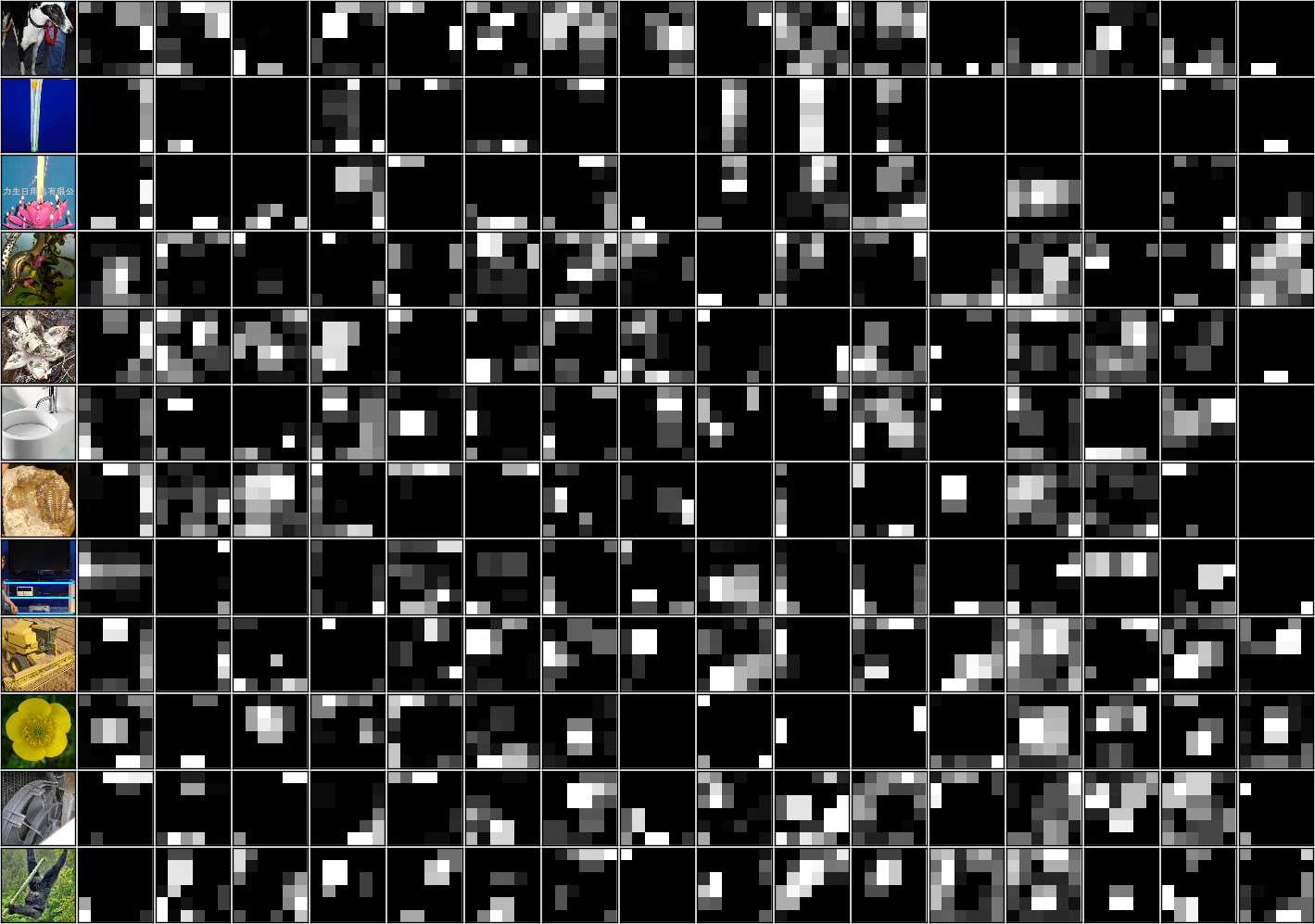
The original supplement supplies feature-map sheets for five convolutional layers and three pooling layers. The leftmost column contains random test images; the remaining columns show a random subset of feature activation maps in the named layer. All eight supplied sheets are retained.
Supplement: classification predictions
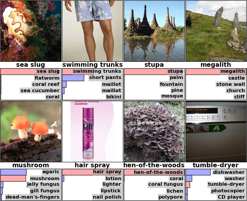
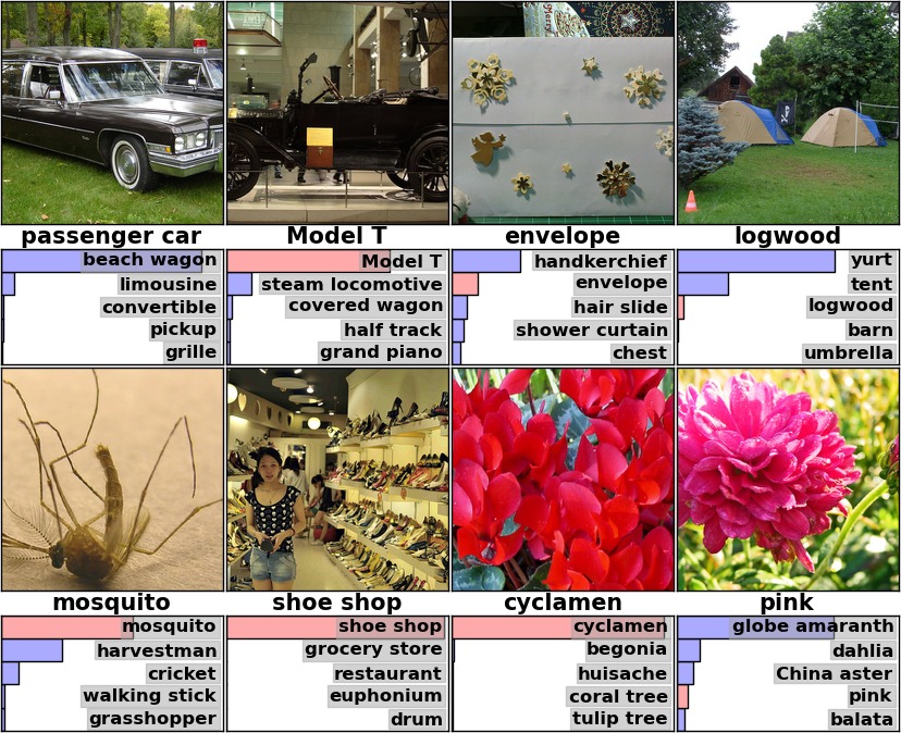
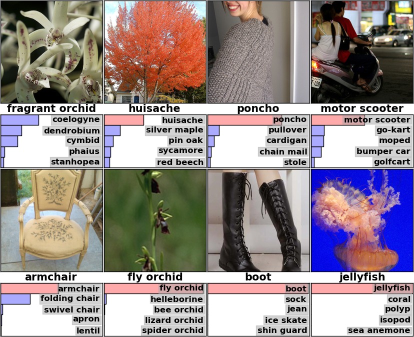
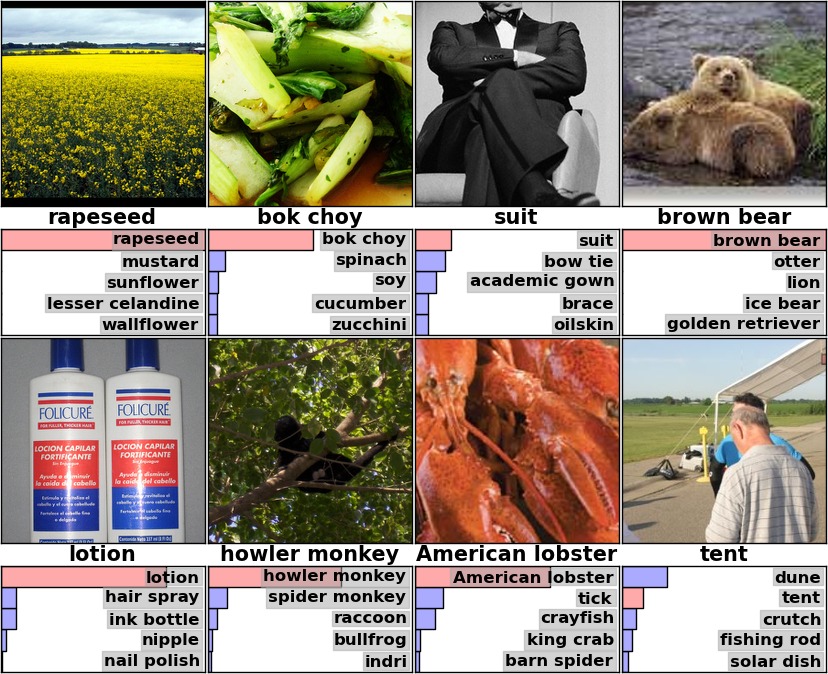
All eleven original prediction sheets are retained. Each image is accompanied by the model’s five most probable labels; a red bar marks the correct category when it appears among those five. The gallery includes successful, ambiguous, and failed examples.
Supplement: nearest-neighbor retrieval
All eight original retrieval sheets are retained. Each first-column test image is followed by the closest training examples under Euclidean distance in the final hidden representation. This displays semantic structure learned from classification labels, without claiming a separately evaluated retrieval system.