Python and numerical arrays
Python containers and functions provide the scaffolding for numerical work; NumPy arrays supply typed, multidimensional storage and vectorized operations. Track array shapes, the difference between slicing and advanced indexing, and the distinction between elementwise multiplication and matrix products. Broadcasting aligns compatible dimensions without writing explicit loops. The retained examples cover scientific utilities and plotting as well as Python syntax. These are the course’s published examples, including historical library APIs, rather than a current installation guide. [26] [27] [32]

def quicksort(arr):
    if len(arr) <= 1:
        return arr
    pivot = arr[len(arr) // 2]
    left = [x for x in arr if x < pivot]
    middle = [x for x in arr if x == pivot]
    right = [x for x in arr if x > pivot]
    return quicksort(left) + middle + quicksort(right)

print(quicksort([3,6,8,10,1,2,1]))
# Prints "[1, 1, 2, 3, 6, 8, 10]"
x = 3
print(type(x)) # Prints "<class 'int'>"
print(x)       # Prints "3"
print(x + 1)   # Addition; prints "4"
print(x - 1)   # Subtraction; prints "2"
print(x * 2)   # Multiplication; prints "6"
print(x ** 2)  # Exponentiation; prints "9"
x += 1
print(x)  # Prints "4"
x *= 2
print(x)  # Prints "8"
y = 2.5
print(type(y)) # Prints "<class 'float'>"
print(y, y + 1, y * 2, y ** 2) # Prints "2.5 3.5 5.0 6.25"
t = True
f = False
print(type(t)) # Prints "<class 'bool'>"
print(t and f) # Logical AND; prints "False"
print(t or f)  # Logical OR; prints "True"
print(not t)   # Logical NOT; prints "False"
print(t != f)  # Logical XOR; prints "True"
hello = 'hello'    # String literals can use single quotes
world = "world"    # or double quotes; it does not matter.
print(hello)       # Prints "hello"
print(len(hello))  # String length; prints "5"
hw = hello + ' ' + world  # String concatenation
print(hw)  # prints "hello world"
hw12 = '%s %s %d' % (hello, world, 12)  # sprintf style string formatting
print(hw12)  # prints "hello world 12"
s = "hello"
print(s.capitalize())  # Capitalize a string; prints "Hello"
print(s.upper())       # Convert a string to uppercase; prints "HELLO"
print(s.rjust(7))      # Right-justify a string, padding with spaces; prints "  hello"
print(s.center(7))     # Center a string, padding with spaces; prints " hello "
print(s.replace('l', '(ell)'))  # Replace all instances of one substring with another;
                                # prints "he(ell)(ell)o"
print('  world '.strip())  # Strip leading and trailing whitespace; prints "world"
xs = [3, 1, 2]    # Create a list
print(xs, xs[2])  # Prints "[3, 1, 2] 2"
print(xs[-1])     # Negative indices count from the end of the list; prints "2"
xs[2] = 'foo'     # Lists can contain elements of different types
print(xs)         # Prints "[3, 1, 'foo']"
xs.append('bar')  # Add a new element to the end of the list
print(xs)         # Prints "[3, 1, 'foo', 'bar']"
x = xs.pop()      # Remove and return the last element of the list
print(x, xs)      # Prints "bar [3, 1, 'foo']"
nums = list(range(5))     # range is a built-in function that creates a list of integers
print(nums)               # Prints "[0, 1, 2, 3, 4]"
print(nums[2:4])          # Get a slice from index 2 to 4 (exclusive); prints "[2, 3]"
print(nums[2:])           # Get a slice from index 2 to the end; prints "[2, 3, 4]"
print(nums[:2])           # Get a slice from the start to index 2 (exclusive); prints "[0, 1]"
print(nums[:])            # Get a slice of the whole list; prints "[0, 1, 2, 3, 4]"
print(nums[:-1])          # Slice indices can be negative; prints "[0, 1, 2, 3]"
nums[2:4] = [8, 9]        # Assign a new sublist to a slice
print(nums)               # Prints "[0, 1, 8, 9, 4]"
animals = ['cat', 'dog', 'monkey']
for animal in animals:
    print(animal)
# Prints "cat", "dog", "monkey", each on its own line.
animals = ['cat', 'dog', 'monkey']
for idx, animal in enumerate(animals):
    print('#%d: %s' % (idx + 1, animal))
# Prints "#1: cat", "#2: dog", "#3: monkey", each on its own line
nums = [0, 1, 2, 3, 4]
squares = []
for x in nums:
    squares.append(x ** 2)
print(squares)   # Prints [0, 1, 4, 9, 16]
nums = [0, 1, 2, 3, 4]
squares = [x ** 2 for x in nums]
print(squares)   # Prints [0, 1, 4, 9, 16]
nums = [0, 1, 2, 3, 4]
even_squares = [x ** 2 for x in nums if x % 2 == 0]
print(even_squares)  # Prints "[0, 4, 16]"
d = {'cat': 'cute', 'dog': 'furry'}  # Create a new dictionary with some data
print(d['cat'])       # Get an entry from a dictionary; prints "cute"
print('cat' in d)     # Check if a dictionary has a given key; prints "True"
d['fish'] = 'wet'     # Set an entry in a dictionary
print(d['fish'])      # Prints "wet"
# print(d['monkey'])  # KeyError: 'monkey' not a key of d
print(d.get('monkey', 'N/A'))  # Get an element with a default; prints "N/A"
print(d.get('fish', 'N/A'))    # Get an element with a default; prints "wet"
del d['fish']         # Remove an element from a dictionary
print(d.get('fish', 'N/A')) # "fish" is no longer a key; prints "N/A"
d = {'person': 2, 'cat': 4, 'spider': 8}
for animal in d:
    legs = d[animal]
    print('A %s has %d legs' % (animal, legs))
# Prints "A person has 2 legs", "A cat has 4 legs", "A spider has 8 legs"
d = {'person': 2, 'cat': 4, 'spider': 8}
for animal, legs in d.items():
    print('A %s has %d legs' % (animal, legs))
# Prints "A person has 2 legs", "A cat has 4 legs", "A spider has 8 legs"
nums = [0, 1, 2, 3, 4]
even_num_to_square = {x: x ** 2 for x in nums if x % 2 == 0}
print(even_num_to_square)  # Prints "{0: 0, 2: 4, 4: 16}"
animals = {'cat', 'dog'}
print('cat' in animals)   # Check if an element is in a set; prints "True"
print('fish' in animals)  # prints "False"
animals.add('fish')       # Add an element to a set
print('fish' in animals)  # Prints "True"
print(len(animals))       # Number of elements in a set; prints "3"
animals.add('cat')        # Adding an element that is already in the set does nothing
print(len(animals))       # Prints "3"
animals.remove('cat')     # Remove an element from a set
print(len(animals))       # Prints "2"
animals = {'cat', 'dog', 'fish'}
for idx, animal in enumerate(animals):
    print('#%d: %s' % (idx + 1, animal))
# Prints "#1: fish", "#2: dog", "#3: cat"
from math import sqrt
nums = {int(sqrt(x)) for x in range(30)}
print(nums)  # Prints "{0, 1, 2, 3, 4, 5}"
d = {(x, x + 1): x for x in range(10)}  # Create a dictionary with tuple keys
t = (5, 6)        # Create a tuple
print(type(t))    # Prints "<class 'tuple'>"
print(d[t])       # Prints "5"
print(d[(1, 2)])  # Prints "1"
def sign(x):
    if x > 0:
        return 'positive'
    elif x < 0:
        return 'negative'
    else:
        return 'zero'

for x in [-1, 0, 1]:
    print(sign(x))
# Prints "negative", "zero", "positive"
def hello(name, loud=False):
    if loud:
        print('HELLO, %s!' % name.upper())
    else:
        print('Hello, %s' % name)

hello('Bob') # Prints "Hello, Bob"
hello('Fred', loud=True)  # Prints "HELLO, FRED!"
class Greeter(object):

    # Constructor
    def __init__(self, name):
        self.name = name  # Create an instance variable

    # Instance method
    def greet(self, loud=False):
        if loud:
            print('HELLO, %s!' % self.name.upper())
        else:
            print('Hello, %s' % self.name)

g = Greeter('Fred')  # Construct an instance of the Greeter class
g.greet()            # Call an instance method; prints "Hello, Fred"
g.greet(loud=True)   # Call an instance method; prints "HELLO, FRED!"
import numpy as np

a = np.array([1, 2, 3])   # Create a rank 1 array
print(type(a))            # Prints "<class 'numpy.ndarray'>"
print(a.shape)            # Prints "(3,)"
print(a[0], a[1], a[2])   # Prints "1 2 3"
a[0] = 5                  # Change an element of the array
print(a)                  # Prints "[5, 2, 3]"

b = np.array([[1,2,3],[4,5,6]])    # Create a rank 2 array
print(b.shape)                     # Prints "(2, 3)"
print(b[0, 0], b[0, 1], b[1, 0])   # Prints "1 2 4"
import numpy as np

a = np.zeros((2,2))   # Create an array of all zeros
print(a)              # Prints "[[ 0.  0.]
                      #          [ 0.  0.]]"

b = np.ones((1,2))    # Create an array of all ones
print(b)              # Prints "[[ 1.  1.]]"

c = np.full((2,2), 7)  # Create a constant array
print(c)               # Prints "[[ 7.  7.]
                       #          [ 7.  7.]]"

d = np.eye(2)         # Create a 2x2 identity matrix
print(d)              # Prints "[[ 1.  0.]
                      #          [ 0.  1.]]"

e = np.random.random((2,2))  # Create an array filled with random values
print(e)                     # Might print "[[ 0.91940167  0.08143941]
                             #               [ 0.68744134  0.87236687]]"
import numpy as np

# Create the following rank 2 array with shape (3, 4)
# [[ 1  2  3  4]
#  [ 5  6  7  8]
#  [ 9 10 11 12]]
a = np.array([[1,2,3,4], [5,6,7,8], [9,10,11,12]])

# Use slicing to pull out the subarray consisting of the first 2 rows
# and columns 1 and 2; b is the following array of shape (2, 2):
# [[2 3]
#  [6 7]]
b = a[:2, 1:3]

# A slice of an array is a view into the same data, so modifying it
# will modify the original array.
print(a[0, 1])   # Prints "2"
b[0, 0] = 77     # b[0, 0] is the same piece of data as a[0, 1]
print(a[0, 1])   # Prints "77"
import numpy as np

# Create the following rank 2 array with shape (3, 4)
# [[ 1  2  3  4]
#  [ 5  6  7  8]
#  [ 9 10 11 12]]
a = np.array([[1,2,3,4], [5,6,7,8], [9,10,11,12]])

# Two ways of accessing the data in the middle row of the array.
# Mixing integer indexing with slices yields an array of lower rank,
# while using only slices yields an array of the same rank as the
# original array:
row_r1 = a[1, :]    # Rank 1 view of the second row of a
row_r2 = a[1:2, :]  # Rank 2 view of the second row of a
print(row_r1, row_r1.shape)  # Prints "[5 6 7 8] (4,)"
print(row_r2, row_r2.shape)  # Prints "[[5 6 7 8]] (1, 4)"

# We can make the same distinction when accessing columns of an array:
col_r1 = a[:, 1]
col_r2 = a[:, 1:2]
print(col_r1, col_r1.shape)  # Prints "[ 2  6 10] (3,)"
print(col_r2, col_r2.shape)  # Prints "[[ 2]
                             #          [ 6]
                             #          [10]] (3, 1)"
import numpy as np

a = np.array([[1,2], [3, 4], [5, 6]])

# An example of integer array indexing.
# The returned array will have shape (3,) and
print(a[[0, 1, 2], [0, 1, 0]])  # Prints "[1 4 5]"

# The above example of integer array indexing is equivalent to this:
print(np.array([a[0, 0], a[1, 1], a[2, 0]]))  # Prints "[1 4 5]"

# When using integer array indexing, you can reuse the same
# element from the source array:
print(a[[0, 0], [1, 1]])  # Prints "[2 2]"

# Equivalent to the previous integer array indexing example
print(np.array([a[0, 1], a[0, 1]]))  # Prints "[2 2]"
import numpy as np

# Create a new array from which we will select elements
a = np.array([[1,2,3], [4,5,6], [7,8,9], [10, 11, 12]])

print(a)  # prints "array([[ 1,  2,  3],
          #                [ 4,  5,  6],
          #                [ 7,  8,  9],
          #                [10, 11, 12]])"

# Create an array of indices
b = np.array([0, 2, 0, 1])

# Select one element from each row of a using the indices in b
print(a[np.arange(4), b])  # Prints "[ 1  6  7 11]"

# Mutate one element from each row of a using the indices in b
a[np.arange(4), b] += 10

print(a)  # prints "array([[11,  2,  3],
          #                [ 4,  5, 16],
          #                [17,  8,  9],
          #                [10, 21, 12]])
import numpy as np

a = np.array([[1,2], [3, 4], [5, 6]])

bool_idx = (a > 2)   # Find the elements of a that are bigger than 2;
                     # this returns a numpy array of Booleans of the same
                     # shape as a, where each slot of bool_idx tells
                     # whether that element of a is > 2.

print(bool_idx)      # Prints "[[False False]
                     #          [ True  True]
                     #          [ True  True]]"

# We use boolean array indexing to construct a rank 1 array
# consisting of the elements of a corresponding to the True values
# of bool_idx
print(a[bool_idx])  # Prints "[3 4 5 6]"

# We can do all of the above in a single concise statement:
print(a[a > 2])     # Prints "[3 4 5 6]"
import numpy as np

x = np.array([1, 2])   # Let numpy choose the datatype
print(x.dtype)         # Prints "int64"

x = np.array([1.0, 2.0])   # Let numpy choose the datatype
print(x.dtype)             # Prints "float64"

x = np.array([1, 2], dtype=np.int64)   # Force a particular datatype
print(x.dtype)                         # Prints "int64"
import numpy as np

x = np.array([[1,2],[3,4]], dtype=np.float64)
y = np.array([[5,6],[7,8]], dtype=np.float64)

# Elementwise sum; both produce the array
# [[ 6.0  8.0]
#  [10.0 12.0]]
print(x + y)
print(np.add(x, y))

# Elementwise difference; both produce the array
# [[-4.0 -4.0]
#  [-4.0 -4.0]]
print(x - y)
print(np.subtract(x, y))

# Elementwise product; both produce the array
# [[ 5.0 12.0]
#  [21.0 32.0]]
print(x * y)
print(np.multiply(x, y))

# Elementwise division; both produce the array
# [[ 0.2         0.33333333]
#  [ 0.42857143  0.5       ]]
print(x / y)
print(np.divide(x, y))

# Elementwise square root; produces the array
# [[ 1.          1.41421356]
#  [ 1.73205081  2.        ]]
print(np.sqrt(x))
import numpy as np

x = np.array([[1,2],[3,4]])
y = np.array([[5,6],[7,8]])

v = np.array([9,10])
w = np.array([11, 12])

# Inner product of vectors; both produce 219
print(v.dot(w))
print(np.dot(v, w))

# Matrix / vector product; both produce the rank 1 array [29 67]
print(x.dot(v))
print(np.dot(x, v))

# Matrix / matrix product; both produce the rank 2 array
# [[19 22]
#  [43 50]]
print(x.dot(y))
print(np.dot(x, y))
import numpy as np

x = np.array([[1,2],[3,4]])

print(np.sum(x))  # Compute sum of all elements; prints "10"
print(np.sum(x, axis=0))  # Compute sum of each column; prints "[4 6]"
print(np.sum(x, axis=1))  # Compute sum of each row; prints "[3 7]"
import numpy as np

x = np.array([[1,2], [3,4]])
print(x)    # Prints "[[1 2]
            #          [3 4]]"
print(x.T)  # Prints "[[1 3]
            #          [2 4]]"

# Note that taking the transpose of a rank 1 array does nothing:
v = np.array([1,2,3])
print(v)    # Prints "[1 2 3]"
print(v.T)  # Prints "[1 2 3]"
import numpy as np

# We will add the vector v to each row of the matrix x,
# storing the result in the matrix y
x = np.array([[1,2,3], [4,5,6], [7,8,9], [10, 11, 12]])
v = np.array([1, 0, 1])
y = np.empty_like(x)   # Create an empty matrix with the same shape as x

# Add the vector v to each row of the matrix x with an explicit loop
for i in range(4):
    y[i, :] = x[i, :] + v

# Now y is the following
# [[ 2  2  4]
#  [ 5  5  7]
#  [ 8  8 10]
#  [11 11 13]]
print(y)
import numpy as np

# We will add the vector v to each row of the matrix x,
# storing the result in the matrix y
x = np.array([[1,2,3], [4,5,6], [7,8,9], [10, 11, 12]])
v = np.array([1, 0, 1])
vv = np.tile(v, (4, 1))   # Stack 4 copies of v on top of each other
print(vv)                 # Prints "[[1 0 1]
                          #          [1 0 1]
                          #          [1 0 1]
                          #          [1 0 1]]"
y = x + vv  # Add x and vv elementwise
print(y)  # Prints "[[ 2  2  4
          #          [ 5  5  7]
          #          [ 8  8 10]
          #          [11 11 13]]"
import numpy as np

# We will add the vector v to each row of the matrix x,
# storing the result in the matrix y
x = np.array([[1,2,3], [4,5,6], [7,8,9], [10, 11, 12]])
v = np.array([1, 0, 1])
y = x + v  # Add v to each row of x using broadcasting
print(y)  # Prints "[[ 2  2  4]
          #          [ 5  5  7]
          #          [ 8  8 10]
          #          [11 11 13]]"
import numpy as np

# Compute outer product of vectors
v = np.array([1,2,3])  # v has shape (3,)
w = np.array([4,5])    # w has shape (2,)
# To compute an outer product, we first reshape v to be a column
# vector of shape (3, 1); we can then broadcast it against w to yield
# an output of shape (3, 2), which is the outer product of v and w:
# [[ 4  5]
#  [ 8 10]
#  [12 15]]
print(np.reshape(v, (3, 1)) * w)

# Add a vector to each row of a matrix
x = np.array([[1,2,3], [4,5,6]])
# x has shape (2, 3) and v has shape (3,) so they broadcast to (2, 3),
# giving the following matrix:
# [[2 4 6]
#  [5 7 9]]
print(x + v)

# Add a vector to each column of a matrix
# x has shape (2, 3) and w has shape (2,).
# If we transpose x then it has shape (3, 2) and can be broadcast
# against w to yield a result of shape (3, 2); transposing this result
# yields the final result of shape (2, 3) which is the matrix x with
# the vector w added to each column. Gives the following matrix:
# [[ 5  6  7]
#  [ 9 10 11]]
print((x.T + w).T)
# Another solution is to reshape w to be a column vector of shape (2, 1);
# we can then broadcast it directly against x to produce the same
# output.
print(x + np.reshape(w, (2, 1)))

# Multiply a matrix by a constant:
# x has shape (2, 3). Numpy treats scalars as arrays of shape ();
# these can be broadcast together to shape (2, 3), producing the
# following array:
# [[ 2  4  6]
#  [ 8 10 12]]
print(x * 2)
from scipy.misc import imread, imsave, imresize

# Read an JPEG image into a numpy array
img = imread('assets/cat.jpg')
print(img.dtype, img.shape)  # Prints "uint8 (400, 248, 3)"

# We can tint the image by scaling each of the color channels
# by a different scalar constant. The image has shape (400, 248, 3);
# we multiply it by the array [1, 0.95, 0.9] of shape (3,);
# numpy broadcasting means that this leaves the red channel unchanged,
# and multiplies the green and blue channels by 0.95 and 0.9
# respectively.
img_tinted = img * [1, 0.95, 0.9]

# Resize the tinted image to be 300 by 300 pixels.
img_tinted = imresize(img_tinted, (300, 300))

# Write the tinted image back to disk
imsave('assets/cat_tinted.jpg', img_tinted)


import numpy as np
from scipy.spatial.distance import pdist, squareform

# Create the following array where each row is a point in 2D space:
# [[0 1]
#  [1 0]
#  [2 0]]
x = np.array([[0, 1], [1, 0], [2, 0]])
print(x)

# Compute the Euclidean distance between all rows of x.
# d[i, j] is the Euclidean distance between x[i, :] and x[j, :],
# and d is the following array:
# [[ 0.          1.41421356  2.23606798]
#  [ 1.41421356  0.          1.        ]
#  [ 2.23606798  1.          0.        ]]
d = squareform(pdist(x, 'euclidean'))
print(d)
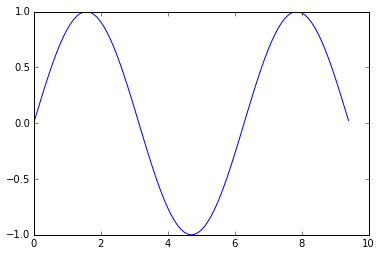
import numpy as np
import matplotlib.pyplot as plt

# Compute the x and y coordinates for points on a sine curve
x = np.arange(0, 3 * np.pi, 0.1)
y = np.sin(x)

# Plot the points using matplotlib
plt.plot(x, y)
plt.show()  # You must call plt.show() to make graphics appear.
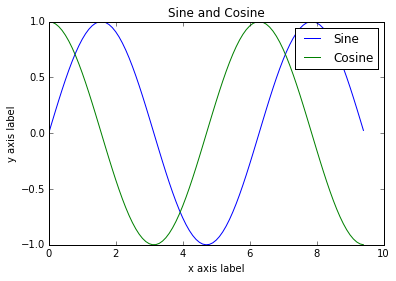
import numpy as np
import matplotlib.pyplot as plt

# Compute the x and y coordinates for points on sine and cosine curves
x = np.arange(0, 3 * np.pi, 0.1)
y_sin = np.sin(x)
y_cos = np.cos(x)

# Plot the points using matplotlib
plt.plot(x, y_sin)
plt.plot(x, y_cos)
plt.xlabel('x axis label')
plt.ylabel('y axis label')
plt.title('Sine and Cosine')
plt.legend(['Sine', 'Cosine'])
plt.show()
import numpy as np
import matplotlib.pyplot as plt

# Compute the x and y coordinates for points on sine and cosine curves
x = np.arange(0, 3 * np.pi, 0.1)
y_sin = np.sin(x)
y_cos = np.cos(x)

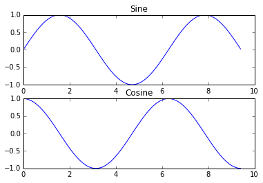
# Set up a subplot grid that has height 2 and width 1,
# and set the first such subplot as active.
plt.subplot(2, 1, 1)

# Make the first plot
plt.plot(x, y_sin)
plt.title('Sine')

# Set the second subplot as active, and make the second plot.
plt.subplot(2, 1, 2)
plt.plot(x, y_cos)
plt.title('Cosine')

# Show the figure.
plt.show()
import numpy as np
from scipy.misc import imread, imresize
import matplotlib.pyplot as plt

img = imread('assets/cat.jpg')
img_tinted = img * [1, 0.95, 0.9]

# Show the original image
plt.subplot(1, 2, 1)
plt.imshow(img)

# Show the tinted image
plt.subplot(1, 2, 2)

# A slight gotcha with imshow is that it might give strange results
# if presented with data that is not uint8. To work around this, we
# explicitly cast the image to uint8 before displaying it.
plt.imshow(np.uint8(img_tinted))
plt.show()
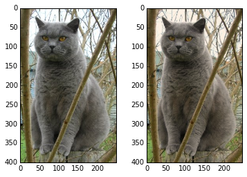
Image classification and nearest neighbors
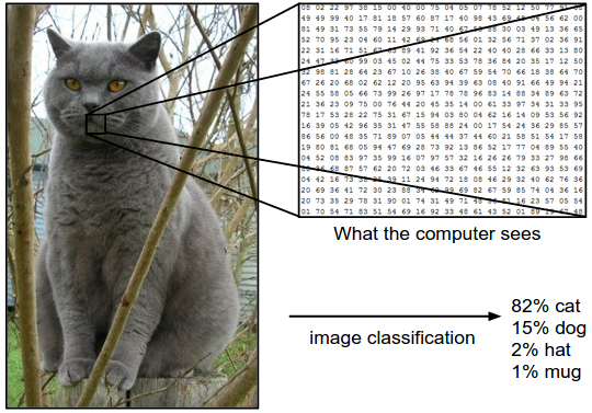
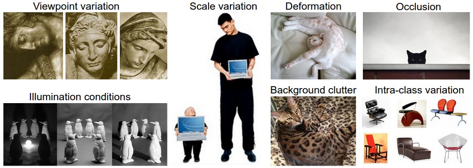
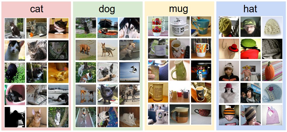
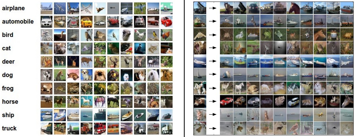
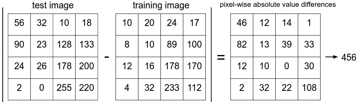
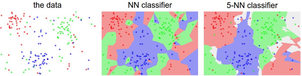
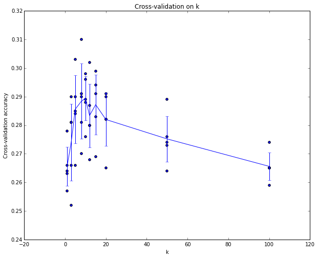
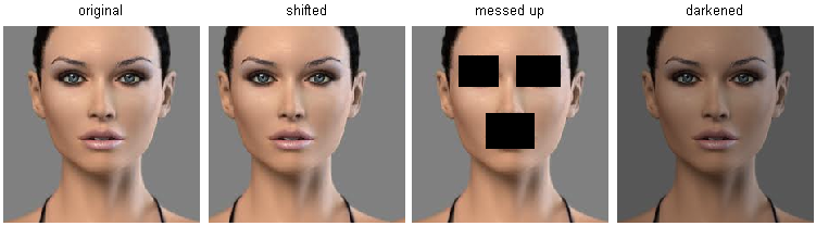
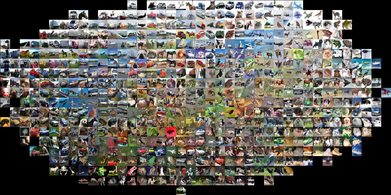
Image classification maps an image to a category using labeled examples. Nearest-neighbor classification makes this data-driven approach explicit, but raw pixel distances are sensitive to nuisance changes and expensive at prediction time. Choose distance measures and the number of neighbors on validation data, keeping the test split untouched until the final evaluation. Cross-validation is useful when data are limited. A baseline’s simplicity is valuable even when its representation is poorly suited to images. [35] [48]
Equation
Xtr, Ytr, Xte, Yte = load_CIFAR10('data/cifar10/') # a magic function we provide
# flatten out all images to be one-dimensional
Xtr_rows = Xtr.reshape(Xtr.shape[0], 32 * 32 * 3) # Xtr_rows becomes 50000 x 3072
Xte_rows = Xte.reshape(Xte.shape[0], 32 * 32 * 3) # Xte_rows becomes 10000 x 3072
nn = NearestNeighbor() # create a Nearest Neighbor classifier class
nn.train(Xtr_rows, Ytr) # train the classifier on the training images and labels
Yte_predict = nn.predict(Xte_rows) # predict labels on the test images
# and now print the classification accuracy, which is the average number
# of examples that are correctly predicted (i.e. label matches)
print 'accuracy: %f' % ( np.mean(Yte_predict == Yte) )
import numpy as np

class NearestNeighbor(object):
  def __init__(self):
    pass

  def train(self, X, y):
    """ X is N x D where each row is an example. Y is 1-dimension of size N """
    # the nearest neighbor classifier simply remembers all the training data
    self.Xtr = X
    self.ytr = y

  def predict(self, X):
    """ X is N x D where each row is an example we wish to predict label for """
    num_test = X.shape[0]
    # lets make sure that the output type matches the input type
    Ypred = np.zeros(num_test, dtype = self.ytr.dtype)

    # loop over all test rows
    for i in range(num_test):
      # find the nearest training image to the i'th test image
      # using the L1 distance (sum of absolute value differences)
      distances = np.sum(np.abs(self.Xtr - X[i,:]), axis = 1)
      min_index = np.argmin(distances) # get the index with smallest distance
      Ypred[i] = self.ytr[min_index] # predict the label of the nearest example

    return Ypred
Equation
distances = np.sqrt(np.sum(np.square(self.Xtr - X[i,:]), axis = 1))
# assume we have Xtr_rows, Ytr, Xte_rows, Yte as before
# recall Xtr_rows is 50,000 x 3072 matrix
Xval_rows = Xtr_rows[:1000, :] # take first 1000 for validation
Yval = Ytr[:1000]
Xtr_rows = Xtr_rows[1000:, :] # keep last 49,000 for train
Ytr = Ytr[1000:]

# find hyperparameters that work best on the validation set
validation_accuracies = []
for k in [1, 3, 5, 10, 20, 50, 100]:

  # use a particular value of k and evaluation on validation data
  nn = NearestNeighbor()
  nn.train(Xtr_rows, Ytr)
  # here we assume a modified NearestNeighbor class that can take a k as input
  Yval_predict = nn.predict(Xval_rows, k = k)
  acc = np.mean(Yval_predict == Yval)
  print 'accuracy: %f' % (acc,)

  # keep track of what works on the validation set
  validation_accuracies.append((k, acc))

Linear classifiers and loss functions
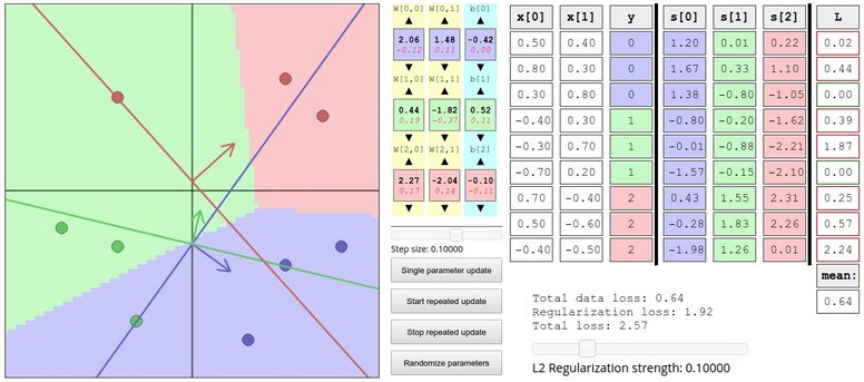
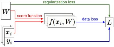
A learned weight matrix and bias map an image vector to class scores. The multiclass hinge objective penalizes insufficient margins, while softmax cross-entropy penalizes low probability assigned to the correct label. Add regularization to control weight magnitude and fit the parameters on training data. Subtracting the largest score before exponentiation stabilizes softmax without changing its probabilities. Linear decision boundaries cannot express arbitrary visual categories, which motivates nonlinear features. [52] [53]
Equation
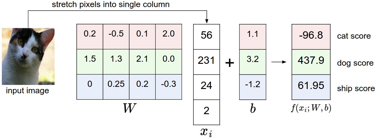
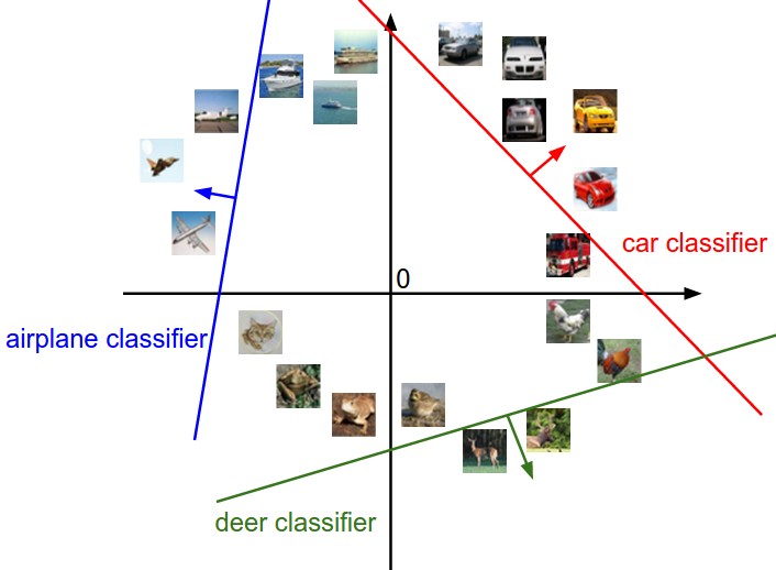

Equations
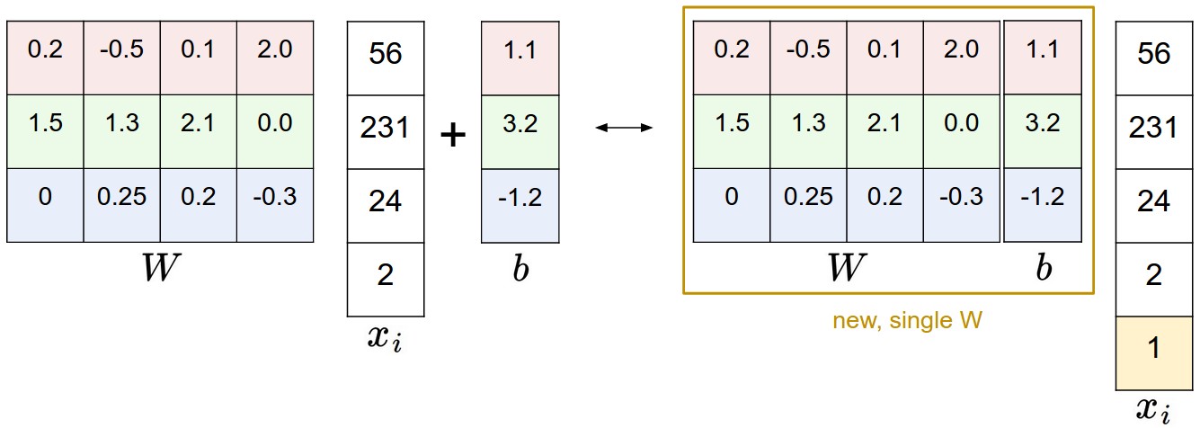
Equations

Equations
def L_i(x, y, W):
  """
  unvectorized version. Compute the multiclass svm loss for a single example (x,y)
  - x is a column vector representing an image (e.g. 3073 x 1 in CIFAR-10)
    with an appended bias dimension in the 3073-rd position (i.e. bias trick)
  - y is an integer giving index of correct class (e.g. between 0 and 9 in CIFAR-10)
  - W is the weight matrix (e.g. 10 x 3073 in CIFAR-10)
  """
  delta = 1.0 # see notes about delta later in this section
  scores = W.dot(x) # scores becomes of size 10 x 1, the scores for each class
  correct_class_score = scores[y]
  D = W.shape[0] # number of classes, e.g. 10
  loss_i = 0.0
  for j in range(D): # iterate over all wrong classes
    if j == y:
      # skip for the true class to only loop over incorrect classes
      continue
    # accumulate loss for the i-th example
    loss_i += max(0, scores[j] - correct_class_score + delta)
  return loss_i

def L_i_vectorized(x, y, W):
  """
  A faster half-vectorized implementation. half-vectorized
  refers to the fact that for a single example the implementation contains
  no for loops, but there is still one loop over the examples (outside this function)
  """
  delta = 1.0
  scores = W.dot(x)
  # compute the margins for all classes in one vector operation
  margins = np.maximum(0, scores - scores[y] + delta)
  # on y-th position scores[y] - scores[y] canceled and gave delta. We want
  # to ignore the y-th position and only consider margin on max wrong class
  margins[y] = 0
  loss_i = np.sum(margins)
  return loss_i

def L(X, y, W):
  """
  fully-vectorized implementation :
  - X holds all the training examples as columns (e.g. 3073 x 50,000 in CIFAR-10)
  - y is array of integers specifying correct class (e.g. 50,000-D array)
  - W are weights (e.g. 10 x 3073)
  """
  # evaluate loss over all examples in X without using any for loops
  # left as exercise to reader in the assignment
Equations
f = np.array([123, 456, 789]) # example with 3 classes and each having large scores
p = np.exp(f) / np.sum(np.exp(f)) # Bad: Numeric problem, potential blowup

# instead: first shift the values of f so that the highest number is 0:
f -= np.max(f) # f becomes [-666, -333, 0]
p = np.exp(f) / np.sum(np.exp(f)) # safe to do, gives the correct answer
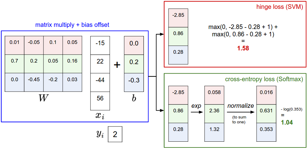
Equations
Optimization and gradient descent
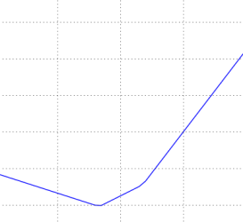
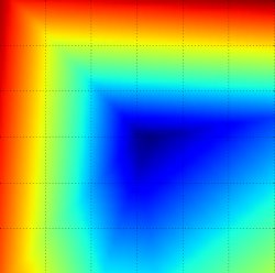
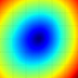
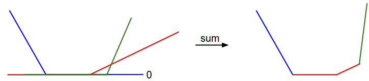
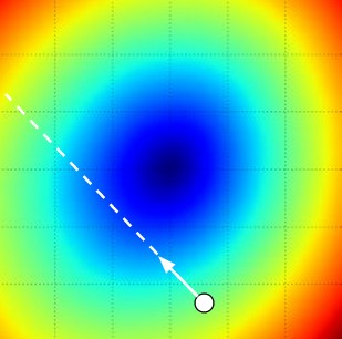
Optimization chooses parameters that reduce the loss. Numerical finite differences approximate gradients and help check an implementation, but analytic derivatives are much cheaper for learning. Gradient descent moves opposite the gradient; minibatches estimate this direction from a subset of examples. Learning rate determines the update size, and an excessively large step can increase the loss even when the direction is locally downhill.
Equation
Equations
# assume X_train is the data where each column is an example (e.g. 3073 x 50,000)
# assume Y_train are the labels (e.g. 1D array of 50,000)
# assume the function L evaluates the loss function

bestloss = float("inf") # Python assigns the highest possible float value
for num in range(1000):
  W = np.random.randn(10, 3073) * 0.0001 # generate random parameters
  loss = L(X_train, Y_train, W) # get the loss over the entire training set
  if loss < bestloss: # keep track of the best solution
    bestloss = loss
    bestW = W
  print 'in attempt %d the loss was %f, best %f' % (num, loss, bestloss)

# prints:
# in attempt 0 the loss was 9.401632, best 9.401632
# in attempt 1 the loss was 8.959668, best 8.959668
# in attempt 2 the loss was 9.044034, best 8.959668
# in attempt 3 the loss was 9.278948, best 8.959668
# in attempt 4 the loss was 8.857370, best 8.857370
# in attempt 5 the loss was 8.943151, best 8.857370
# in attempt 6 the loss was 8.605604, best 8.605604
# ... (trunctated: continues for 1000 lines)
# Assume X_test is [3073 x 10000], Y_test [10000 x 1]
scores = Wbest.dot(Xte_cols) # 10 x 10000, the class scores for all test examples
# find the index with max score in each column (the predicted class)
Yte_predict = np.argmax(scores, axis = 0)
# and calculate accuracy (fraction of predictions that are correct)
np.mean(Yte_predict == Yte)
# returns 0.1555
W = np.random.randn(10, 3073) * 0.001 # generate random starting W
bestloss = float("inf")
for i in range(1000):
  step_size = 0.0001
  Wtry = W + np.random.randn(10, 3073) * step_size
  loss = L(Xtr_cols, Ytr, Wtry)
  if loss < bestloss:
    W = Wtry
    bestloss = loss
  print 'iter %d loss is %f' % (i, bestloss)
Equation
def eval_numerical_gradient(f, x):
  """
  a naive implementation of numerical gradient of f at x
  - f should be a function that takes a single argument
  - x is the point (numpy array) to evaluate the gradient at
  """

  fx = f(x) # evaluate function value at original point
  grad = np.zeros(x.shape)
  h = 0.00001

  # iterate over all indexes in x
  it = np.nditer(x, flags=['multi_index'], op_flags=['readwrite'])
  while not it.finished:

    # evaluate function at x+h
    ix = it.multi_index
    old_value = x[ix]
    x[ix] = old_value + h # increment by h
    fxh = f(x) # evalute f(x + h)
    x[ix] = old_value # restore to previous value (very important!)

    # compute the partial derivative
    grad[ix] = (fxh - fx) / h # the slope
    it.iternext() # step to next dimension

  return grad
# to use the generic code above we want a function that takes a single argument
# (the weights in our case) so we close over X_train and Y_train
def CIFAR10_loss_fun(W):
  return L(X_train, Y_train, W)

W = np.random.rand(10, 3073) * 0.001 # random weight vector
df = eval_numerical_gradient(CIFAR10_loss_fun, W) # get the gradient
loss_original = CIFAR10_loss_fun(W) # the original loss
print 'original loss: %f' % (loss_original, )

# lets see the effect of multiple step sizes
for step_size_log in [-10, -9, -8, -7, -6, -5,-4,-3,-2,-1]:
  step_size = 10 ** step_size_log
  W_new = W - step_size * df # new position in the weight space
  loss_new = CIFAR10_loss_fun(W_new)
  print 'for step size %f new loss: %f' % (step_size, loss_new)

# prints:
# original loss: 2.200718
# for step size 1.000000e-10 new loss: 2.200652
# for step size 1.000000e-09 new loss: 2.200057
# for step size 1.000000e-08 new loss: 2.194116
# for step size 1.000000e-07 new loss: 2.135493
# for step size 1.000000e-06 new loss: 1.647802
# for step size 1.000000e-05 new loss: 2.844355
# for step size 1.000000e-04 new loss: 25.558142
# for step size 1.000000e-03 new loss: 254.086573
# for step size 1.000000e-02 new loss: 2539.370888
# for step size 1.000000e-01 new loss: 25392.214036
Equations
# Vanilla Gradient Descent

while True:
  weights_grad = evaluate_gradient(loss_fun, data, weights)
  weights += - step_size * weights_grad # perform parameter update
# Vanilla Minibatch Gradient Descent

while True:
  data_batch = sample_training_data(data, 256) # sample 256 examples
  weights_grad = evaluate_gradient(loss_fun, data_batch, weights)
  weights += - step_size * weights_grad # perform parameter update
Backpropagation
Backpropagation evaluates local derivatives along a computation graph and combines them with the chain rule. Cache intermediate values in the forward pass, then propagate upstream sensitivities backward, adding contributions when a value has multiple downstream uses. Addition distributes gradients, multiplication scales them by the other operand, and a maximum routes them through the selected input. Vectorized derivatives require careful attention to dimensions and transposes. The original computational graphs and staged code examples are preserved. [58] [59]
Equations
# set some inputs
x = -2; y = 5; z = -4

# perform the forward pass
q = x + y # q becomes 3
f = q * z # f becomes -12

# perform the backward pass (backpropagation) in reverse order:
# first backprop through f = q * z
dfdz = q # df/dz = q, so gradient on z becomes 3
dfdq = z # df/dq = z, so gradient on q becomes -4
dqdx = 1.0
dqdy = 1.0
# now backprop through q = x + y
dfdx = dfdq * dqdx  # The multiplication here is the chain rule!
dfdy = dfdq * dqdy
Equations
Equation
w = [2,-3,-3] # assume some random weights and data
x = [-1, -2]

# forward pass
dot = w[0]*x[0] + w[1]*x[1] + w[2]
f = 1.0 / (1 + math.exp(-dot)) # sigmoid function

# backward pass through the neuron (backpropagation)
ddot = (1 - f) * f # gradient on dot variable, using the sigmoid gradient derivation
dx = [w[0] * ddot, w[1] * ddot] # backprop into x
dw = [x[0] * ddot, x[1] * ddot, 1.0 * ddot] # backprop into w
# we're done! we have the gradients on the inputs to the circuit
Equation
x = 3 # example values
y = -4

# forward pass
sigy = 1.0 / (1 + math.exp(-y)) # sigmoid in numerator   #(1)
num = x + sigy # numerator                               #(2)
sigx = 1.0 / (1 + math.exp(-x)) # sigmoid in denominator #(3)
xpy = x + y                                              #(4)
xpysqr = xpy**2                                          #(5)
den = sigx + xpysqr # denominator                        #(6)
invden = 1.0 / den                                       #(7)
f = num * invden # done!                                 #(8)
# backprop f = num * invden
dnum = invden # gradient on numerator                             #(8)
dinvden = num                                                     #(8)
# backprop invden = 1.0 / den
dden = (-1.0 / (den**2)) * dinvden                                #(7)
# backprop den = sigx + xpysqr
dsigx = (1) * dden                                                #(6)
dxpysqr = (1) * dden                                              #(6)
# backprop xpysqr = xpy**2
dxpy = (2 * xpy) * dxpysqr                                        #(5)
# backprop xpy = x + y
dx = (1) * dxpy                                                   #(4)
dy = (1) * dxpy                                                   #(4)
# backprop sigx = 1.0 / (1 + math.exp(-x))
dx += ((1 - sigx) * sigx) * dsigx # Notice += !! See notes below  #(3)
# backprop num = x + sigy
dx += (1) * dnum                                                  #(2)
dsigy = (1) * dnum                                                #(2)
# backprop sigy = 1.0 / (1 + math.exp(-y))
dy += ((1 - sigy) * sigy) * dsigy                                 #(1)
# done! phew
# forward pass
W = np.random.randn(5, 10)
X = np.random.randn(10, 3)
D = W.dot(X)

# now suppose we had the gradient on D from above in the circuit
dD = np.random.randn(*D.shape) # same shape as D
dW = dD.dot(X.T) #.T gives the transpose of the matrix
dX = W.T.dot(dD)
Network architecture and activations
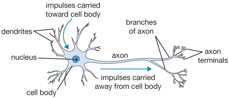
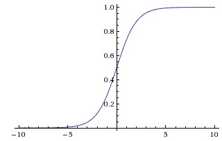
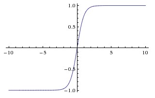
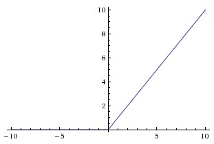
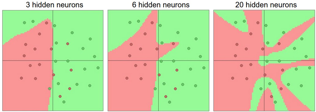
Alternating affine transformations and nonlinear activations creates a network whose capacity exceeds a linear classifier. The notes compare sigmoid, tanh, and rectified activations, including saturation and inactive-unit problems. Universal approximation describes representational capacity; it does not guarantee that finite data or optimization will recover the desired function. Depth, width, regularization, and validation performance jointly guide architecture choice. [65] [69]
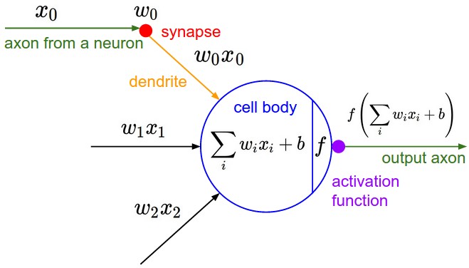
class Neuron(object):
  # ...
  def forward(self, inputs):
    """ assume inputs and weights are 1-D numpy arrays and bias is a number """
    cell_body_sum = np.sum(inputs * self.weights) + self.bias
    firing_rate = 1.0 / (1.0 + math.exp(-cell_body_sum)) # sigmoid activation function
    return firing_rate
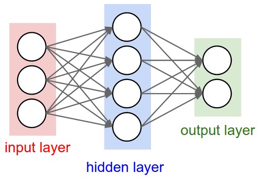
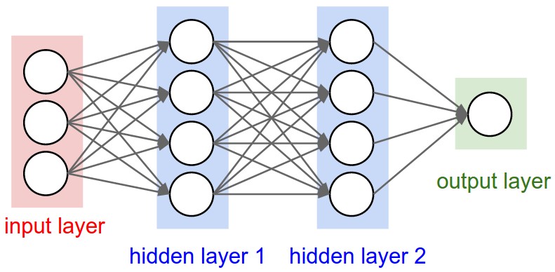
# forward-pass of a 3-layer neural network:
f = lambda x: 1.0/(1.0 + np.exp(-x)) # activation function (use sigmoid)
x = np.random.randn(3, 1) # random input vector of three numbers (3x1)
h1 = f(np.dot(W1, x) + b1) # calculate first hidden layer activations (4x1)
h2 = f(np.dot(W2, h1) + b2) # calculate second hidden layer activations (4x1)
out = np.dot(W3, h2) + b3 # output neuron (1x1)
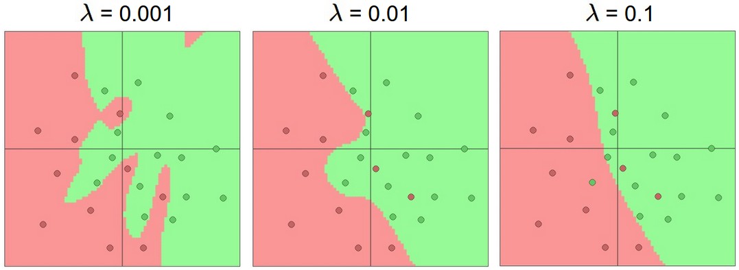
Data, initialization, and regularization
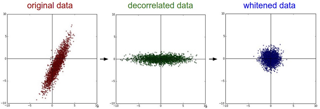
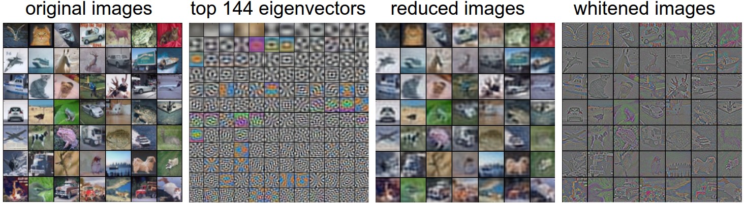
Estimate preprocessing statistics using training data, then apply the same transformation to validation and test inputs. Centering, scaling, decorrelation, and whitening serve different purposes. Initialization should break symmetry while maintaining useful signal and gradient scales. Regularization options include weight penalties, dropout, and related constraints. Choose a data loss that matches classification, regression, or another target, and add it to the regularization term. [79] [83]
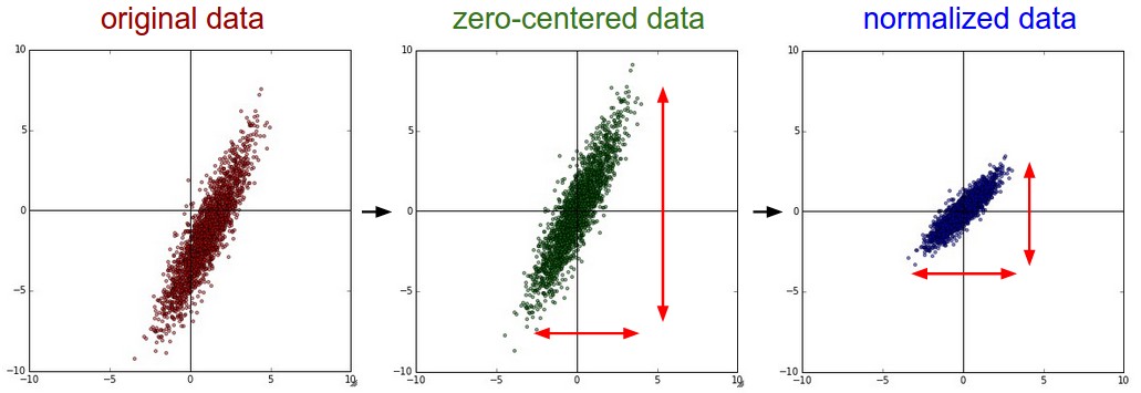
# Assume input data matrix X of size [N x D]
X -= np.mean(X, axis = 0) # zero-center the data (important)
cov = np.dot(X.T, X) / X.shape[0] # get the data covariance matrix
U,S,V = np.linalg.svd(cov)
Xrot = np.dot(X, U) # decorrelate the data
Xrot_reduced = np.dot(X, U[:,:100]) # Xrot_reduced becomes [N x 100]
# whiten the data:
# divide by the eigenvalues (which are square roots of the singular values)
Xwhite = Xrot / np.sqrt(S + 1e-5)
Equation
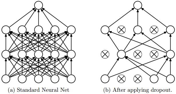
""" Vanilla Dropout: Not recommended implementation (see notes below) """

p = 0.5 # probability of keeping a unit active. higher = less dropout

def train_step(X):
  """ X contains the data """

  # forward pass for example 3-layer neural network
  H1 = np.maximum(0, np.dot(W1, X) + b1)
  U1 = np.random.rand(*H1.shape) < p # first dropout mask
  H1 *= U1 # drop!
  H2 = np.maximum(0, np.dot(W2, H1) + b2)
  U2 = np.random.rand(*H2.shape) < p # second dropout mask
  H2 *= U2 # drop!
  out = np.dot(W3, H2) + b3

  # backward pass: compute gradients... (not shown)
  # perform parameter update... (not shown)

def predict(X):
  # ensembled forward pass
  H1 = np.maximum(0, np.dot(W1, X) + b1) * p # NOTE: scale the activations
  H2 = np.maximum(0, np.dot(W2, H1) + b2) * p # NOTE: scale the activations
  out = np.dot(W3, H2) + b3
"""
Inverted Dropout: Recommended implementation example.
We drop and scale at train time and don't do anything at test time.
"""

p = 0.5 # probability of keeping a unit active. higher = less dropout

def train_step(X):
  # forward pass for example 3-layer neural network
  H1 = np.maximum(0, np.dot(W1, X) + b1)
  U1 = (np.random.rand(*H1.shape) < p) / p # first dropout mask. Notice /p!
  H1 *= U1 # drop!
  H2 = np.maximum(0, np.dot(W2, H1) + b2)
  U2 = (np.random.rand(*H2.shape) < p) / p # second dropout mask. Notice /p!
  H2 *= U2 # drop!
  out = np.dot(W3, H2) + b3

  # backward pass: compute gradients... (not shown)
  # perform parameter update... (not shown)

def predict(X):
  # ensembled forward pass
  H1 = np.maximum(0, np.dot(W1, X) + b1) # no scaling necessary
  H2 = np.maximum(0, np.dot(W2, H1) + b2)
  out = np.dot(W3, H2) + b3
Equations
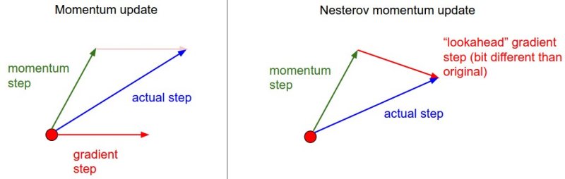
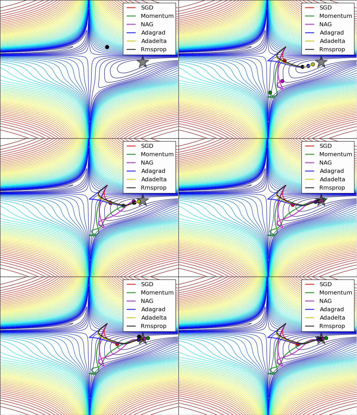
Training and evaluation
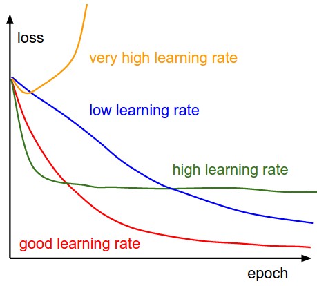
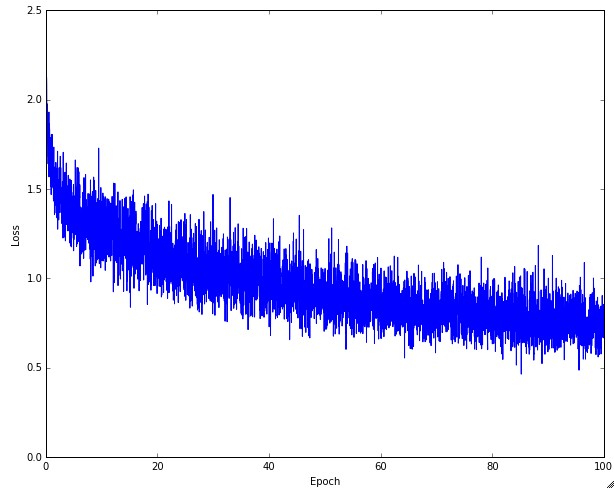
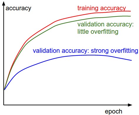
Before a long run, check gradients and initial loss, and verify that a small dataset can be overfit. Monitor training and validation accuracy, loss, update-to-weight ratios, and activation or gradient distributions. Compare stochastic gradient descent, momentum, adaptive methods, and learning-rate schedules. Search hyperparameters on validation data, often over logarithmic scales; model ensembles can improve predictions at additional cost. The plots illustrate diagnostic patterns rather than universal numerical thresholds. [98] [101]
Equations
# assume parameter vector W and its gradient vector dW
param_scale = np.linalg.norm(W.ravel())
update = -learning_rate*dW # simple SGD update
update_scale = np.linalg.norm(update.ravel())
W += update # the actual update
print update_scale / param_scale # want ~1e-3
# Vanilla update
x += - learning_rate * dx
# Momentum update
v = mu * v - learning_rate * dx # integrate velocity
x += v # integrate position
x_ahead = x + mu * v
# evaluate dx_ahead (the gradient at x_ahead instead of at x)
v = mu * v - learning_rate * dx_ahead
x += v
v_prev = v # back this up
v = mu * v - learning_rate * dx # velocity update stays the same
x += -mu * v_prev + (1 + mu) * v # position update changes form
Equation
# Assume the gradient dx and parameter vector x
cache += dx**2
x += - learning_rate * dx / (np.sqrt(cache) + eps)
cache = decay_rate * cache + (1 - decay_rate) * dx**2
x += - learning_rate * dx / (np.sqrt(cache) + eps)
m = beta1*m + (1-beta1)*dx
v = beta2*v + (1-beta2)*(dx**2)
x += - learning_rate * m / (np.sqrt(v) + eps)
# t is your iteration counter going from 1 to infinity
m = beta1*m + (1-beta1)*dx
mt = m / (1-beta1**t)
v = beta2*v + (1-beta2)*(dx**2)
vt = v / (1-beta2**t)
x += - learning_rate * mt / (np.sqrt(vt) + eps)
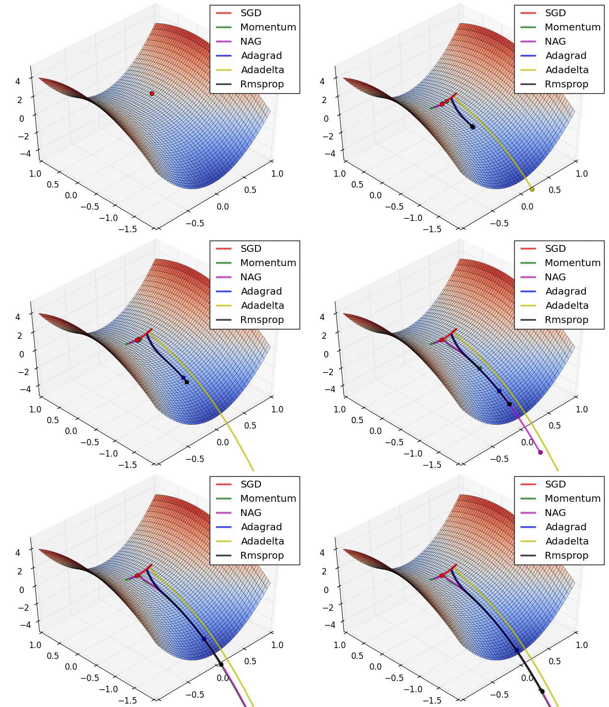
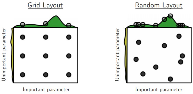
A minimal classification network
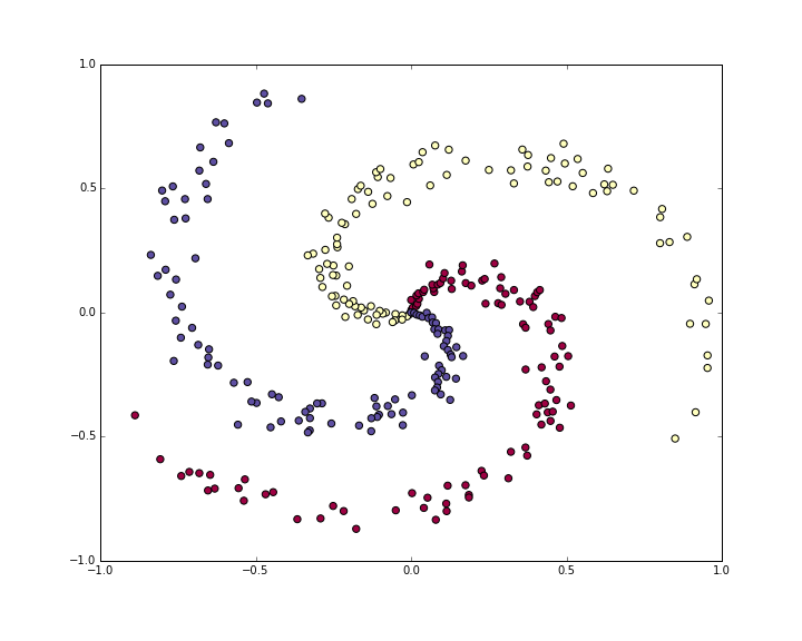
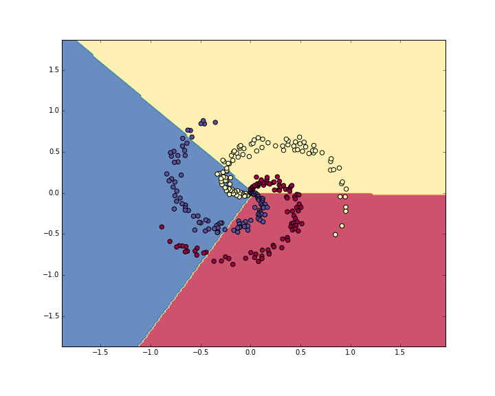
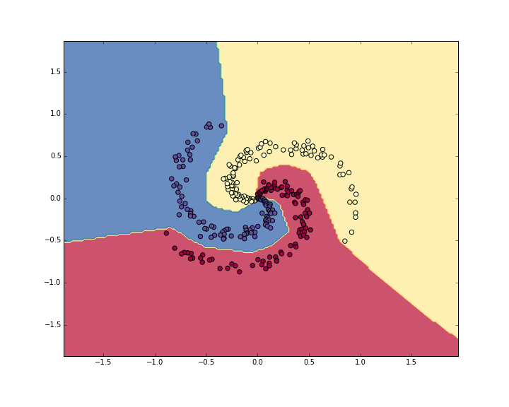
A spiral dataset exposes the limits of a linear softmax classifier. Adding one nonlinear hidden layer changes the decision boundary enough to fit the toy task. The complete code follows scores, normalized probabilities, regularized cross-entropy, analytic gradients, and parameter updates, making the connection between the equations and implementation explicit.
N = 100 # number of points per class
D = 2 # dimensionality
K = 3 # number of classes
X = np.zeros((N*K,D)) # data matrix (each row = single example)
y = np.zeros(N*K, dtype='uint8') # class labels
for j in range(K):
  ix = range(N*j,N*(j+1))
  r = np.linspace(0.0,1,N) # radius
  t = np.linspace(j*4,(j+1)*4,N) + np.random.randn(N)*0.2 # theta
  X[ix] = np.c_[r*np.sin(t), r*np.cos(t)]
  y[ix] = j
# lets visualize the data:
plt.scatter(X[:, 0], X[:, 1], c=y, s=40, cmap=plt.cm.Spectral)
plt.show()
# initialize parameters randomly
W = 0.01 * np.random.randn(D,K)
b = np.zeros((1,K))
# compute class scores for a linear classifier
scores = np.dot(X, W) + b
Equations
num_examples = X.shape[0]
# get unnormalized probabilities
exp_scores = np.exp(scores)
# normalize them for each example
probs = exp_scores / np.sum(exp_scores, axis=1, keepdims=True)
correct_logprobs = -np.log(probs[range(num_examples),y])
# compute the loss: average cross-entropy loss and regularization
data_loss = np.sum(correct_logprobs)/num_examples
reg_loss = 0.5*reg*np.sum(W*W)
loss = data_loss + reg_loss
Equations
dscores = probs
dscores[range(num_examples),y] -= 1
dscores /= num_examples
dW = np.dot(X.T, dscores)
db = np.sum(dscores, axis=0, keepdims=True)
dW += reg*W # don't forget the regularization gradient
# perform a parameter update
W += -step_size * dW
b += -step_size * db
#Train a Linear Classifier

# initialize parameters randomly
W = 0.01 * np.random.randn(D,K)
b = np.zeros((1,K))

# some hyperparameters
step_size = 1e-0
reg = 1e-3 # regularization strength

# gradient descent loop
num_examples = X.shape[0]
for i in range(200):

  # evaluate class scores, [N x K]
  scores = np.dot(X, W) + b

  # compute the class probabilities
  exp_scores = np.exp(scores)
  probs = exp_scores / np.sum(exp_scores, axis=1, keepdims=True) # [N x K]

  # compute the loss: average cross-entropy loss and regularization
  correct_logprobs = -np.log(probs[range(num_examples),y])
  data_loss = np.sum(correct_logprobs)/num_examples
  reg_loss = 0.5*reg*np.sum(W*W)
  loss = data_loss + reg_loss
  if i % 10 == 0:
    print "iteration %d: loss %f" % (i, loss)

  # compute the gradient on scores
  dscores = probs
  dscores[range(num_examples),y] -= 1
  dscores /= num_examples

  # backpropate the gradient to the parameters (W,b)
  dW = np.dot(X.T, dscores)
  db = np.sum(dscores, axis=0, keepdims=True)

  dW += reg*W # regularization gradient

  # perform a parameter update
  W += -step_size * dW
  b += -step_size * db
iteration 0: loss 1.096956
iteration 10: loss 0.917265
iteration 20: loss 0.851503
iteration 30: loss 0.822336
iteration 40: loss 0.807586
iteration 50: loss 0.799448
iteration 60: loss 0.794681
iteration 70: loss 0.791764
iteration 80: loss 0.789920
iteration 90: loss 0.788726
iteration 100: loss 0.787938
iteration 110: loss 0.787409
iteration 120: loss 0.787049
iteration 130: loss 0.786803
iteration 140: loss 0.786633
iteration 150: loss 0.786514
iteration 160: loss 0.786431
iteration 170: loss 0.786373
iteration 180: loss 0.786331
iteration 190: loss 0.786302
# evaluate training set accuracy
scores = np.dot(X, W) + b
predicted_class = np.argmax(scores, axis=1)
print 'training accuracy: %.2f' % (np.mean(predicted_class == y))
# initialize parameters randomly
h = 100 # size of hidden layer
W = 0.01 * np.random.randn(D,h)
b = np.zeros((1,h))
W2 = 0.01 * np.random.randn(h,K)
b2 = np.zeros((1,K))
# evaluate class scores with a 2-layer Neural Network
hidden_layer = np.maximum(0, np.dot(X, W) + b) # note, ReLU activation
scores = np.dot(hidden_layer, W2) + b2
# backpropate the gradient to the parameters
# first backprop into parameters W2 and b2
dW2 = np.dot(hidden_layer.T, dscores)
db2 = np.sum(dscores, axis=0, keepdims=True)
dhidden = np.dot(dscores, W2.T)
# backprop the ReLU non-linearity
dhidden[hidden_layer <= 0] = 0
# finally into W,b
dW = np.dot(X.T, dhidden)
db = np.sum(dhidden, axis=0, keepdims=True)
# initialize parameters randomly
h = 100 # size of hidden layer
W = 0.01 * np.random.randn(D,h)
b = np.zeros((1,h))
W2 = 0.01 * np.random.randn(h,K)
b2 = np.zeros((1,K))

# some hyperparameters
step_size = 1e-0
reg = 1e-3 # regularization strength

# gradient descent loop
num_examples = X.shape[0]
for i in range(10000):

  # evaluate class scores, [N x K]
  hidden_layer = np.maximum(0, np.dot(X, W) + b) # note, ReLU activation
  scores = np.dot(hidden_layer, W2) + b2

  # compute the class probabilities
  exp_scores = np.exp(scores)
  probs = exp_scores / np.sum(exp_scores, axis=1, keepdims=True) # [N x K]

  # compute the loss: average cross-entropy loss and regularization
  correct_logprobs = -np.log(probs[range(num_examples),y])
  data_loss = np.sum(correct_logprobs)/num_examples
  reg_loss = 0.5*reg*np.sum(W*W) + 0.5*reg*np.sum(W2*W2)
  loss = data_loss + reg_loss
  if i % 1000 == 0:
    print "iteration %d: loss %f" % (i, loss)

  # compute the gradient on scores
  dscores = probs
  dscores[range(num_examples),y] -= 1
  dscores /= num_examples

  # backpropate the gradient to the parameters
  # first backprop into parameters W2 and b2
  dW2 = np.dot(hidden_layer.T, dscores)
  db2 = np.sum(dscores, axis=0, keepdims=True)
  # next backprop into hidden layer
  dhidden = np.dot(dscores, W2.T)
  # backprop the ReLU non-linearity
  dhidden[hidden_layer <= 0] = 0
  # finally into W,b
  dW = np.dot(X.T, dhidden)
  db = np.sum(dhidden, axis=0, keepdims=True)

  # add regularization gradient contribution
  dW2 += reg * W2
  dW += reg * W

  # perform a parameter update
  W += -step_size * dW
  b += -step_size * db
  W2 += -step_size * dW2
  b2 += -step_size * db2
iteration 0: loss 1.098744
iteration 1000: loss 0.294946
iteration 2000: loss 0.259301
iteration 3000: loss 0.248310
iteration 4000: loss 0.246170
iteration 5000: loss 0.245649
iteration 6000: loss 0.245491
iteration 7000: loss 0.245400
iteration 8000: loss 0.245335
iteration 9000: loss 0.245292
# evaluate training set accuracy
hidden_layer = np.maximum(0, np.dot(X, W) + b)
scores = np.dot(hidden_layer, W2) + b2
predicted_class = np.argmax(scores, axis=1)
print 'training accuracy: %.2f' % (np.mean(predicted_class == y))
Convolutional networks
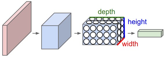
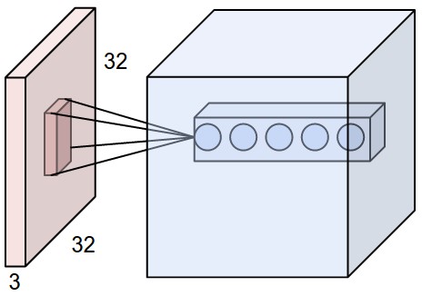
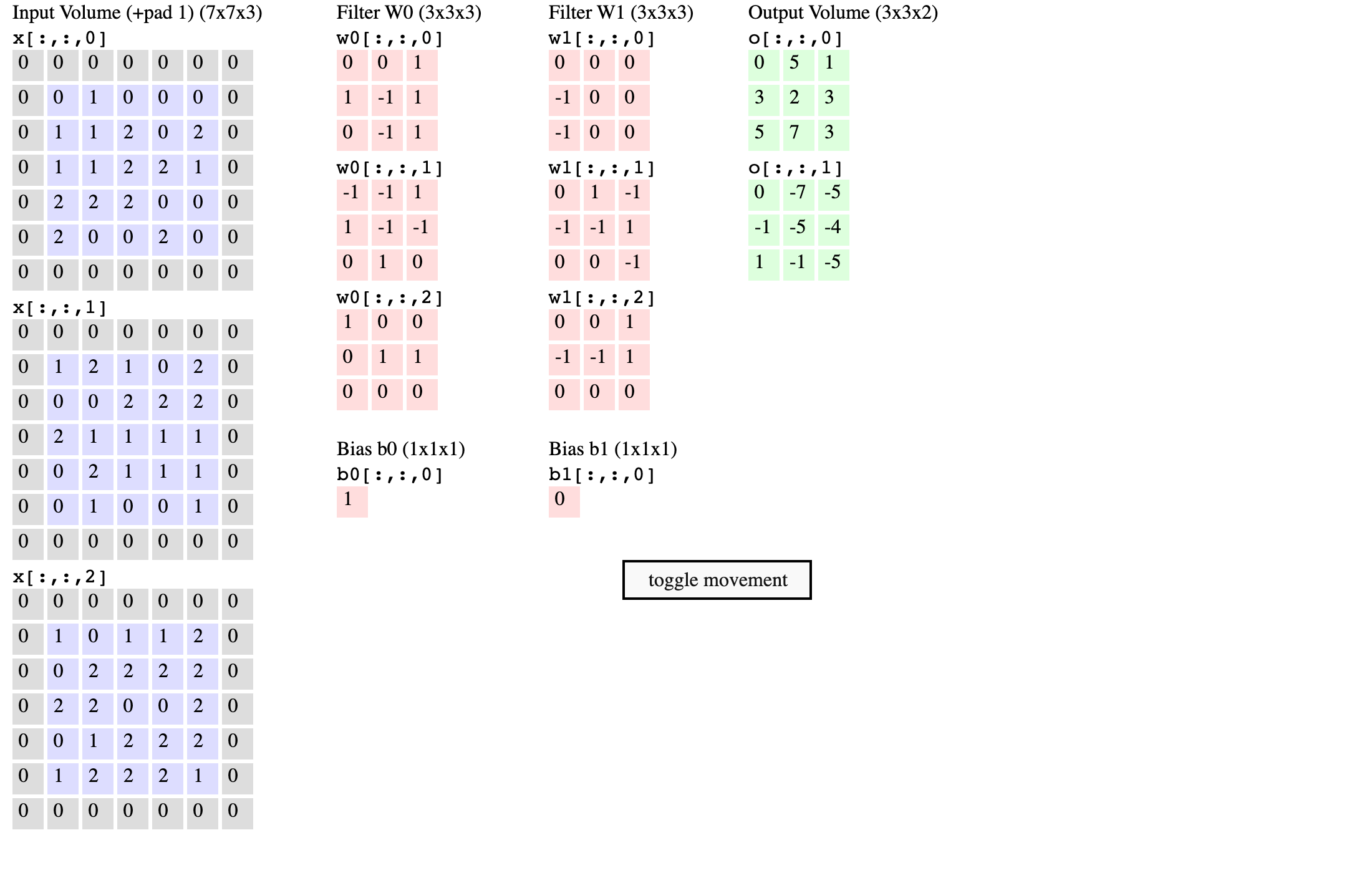
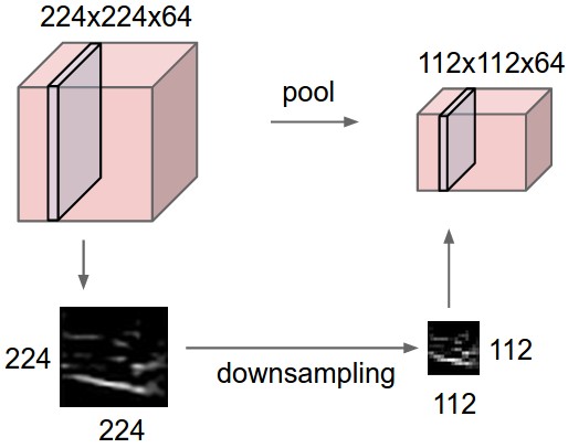
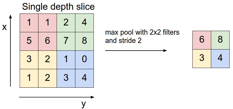
Convolution combines local receptive fields with weights shared across spatial positions. Filter size, padding, stride, and channel count determine output geometry and parameter count; pooling changes spatial resolution. Fully connected operations can be rewritten as convolutions when their shapes are matched. The notes compare named architectures and explain activation-memory costs during training. The embedded convolution example is retained as a static illustration with a link to its interactive controls. Hardware capacities and architecture recommendations reflect the historical notes. [113] [128] [132]
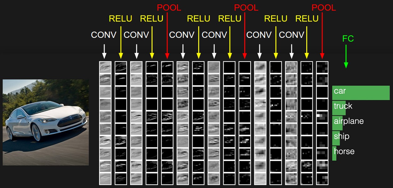

INPUT: [224x224x3]        memory:  224*224*3=150K   weights: 0
CONV3-64: [224x224x64]  memory:  224*224*64=3.2M   weights: (3*3*3)*64 = 1,728
CONV3-64: [224x224x64]  memory:  224*224*64=3.2M   weights: (3*3*64)*64 = 36,864
POOL2: [112x112x64]  memory:  112*112*64=800K   weights: 0
CONV3-128: [112x112x128]  memory:  112*112*128=1.6M   weights: (3*3*64)*128 = 73,728
CONV3-128: [112x112x128]  memory:  112*112*128=1.6M   weights: (3*3*128)*128 = 147,456
POOL2: [56x56x128]  memory:  56*56*128=400K   weights: 0
CONV3-256: [56x56x256]  memory:  56*56*256=800K   weights: (3*3*128)*256 = 294,912
CONV3-256: [56x56x256]  memory:  56*56*256=800K   weights: (3*3*256)*256 = 589,824
CONV3-256: [56x56x256]  memory:  56*56*256=800K   weights: (3*3*256)*256 = 589,824
POOL2: [28x28x256]  memory:  28*28*256=200K   weights: 0
CONV3-512: [28x28x512]  memory:  28*28*512=400K   weights: (3*3*256)*512 = 1,179,648
CONV3-512: [28x28x512]  memory:  28*28*512=400K   weights: (3*3*512)*512 = 2,359,296
CONV3-512: [28x28x512]  memory:  28*28*512=400K   weights: (3*3*512)*512 = 2,359,296
POOL2: [14x14x512]  memory:  14*14*512=100K   weights: 0
CONV3-512: [14x14x512]  memory:  14*14*512=100K   weights: (3*3*512)*512 = 2,359,296
CONV3-512: [14x14x512]  memory:  14*14*512=100K   weights: (3*3*512)*512 = 2,359,296
CONV3-512: [14x14x512]  memory:  14*14*512=100K   weights: (3*3*512)*512 = 2,359,296
POOL2: [7x7x512]  memory:  7*7*512=25K  weights: 0
FC: [1x1x4096]  memory:  4096  weights: 7*7*512*4096 = 102,760,448
FC: [1x1x4096]  memory:  4096  weights: 4096*4096 = 16,777,216
FC: [1x1x1000]  memory:  1000 weights: 4096*1000 = 4,096,000

TOTAL memory: 24M * 4 bytes ~= 93MB / image (only forward! ~*2 for bwd)
TOTAL params: 138M parameters
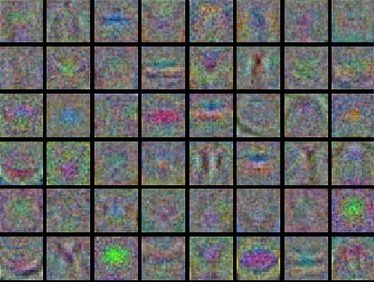
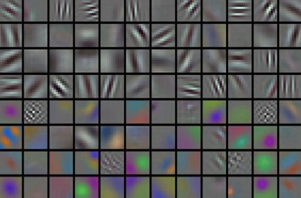
Inspecting learned representations
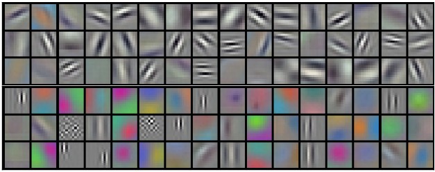
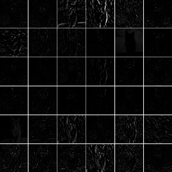
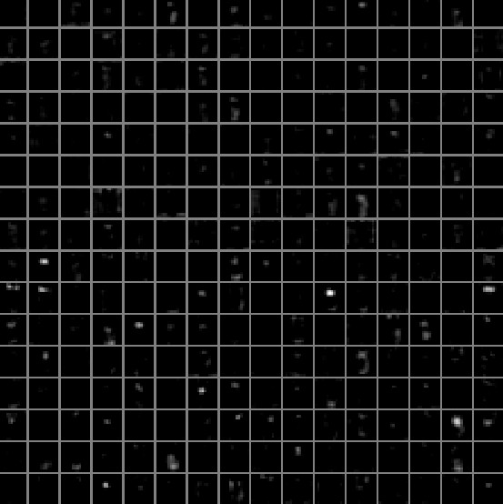
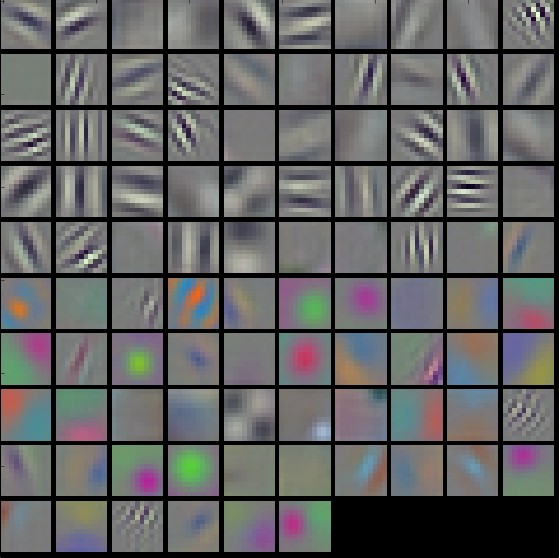
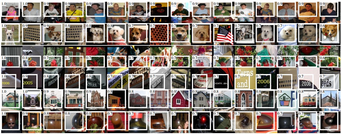
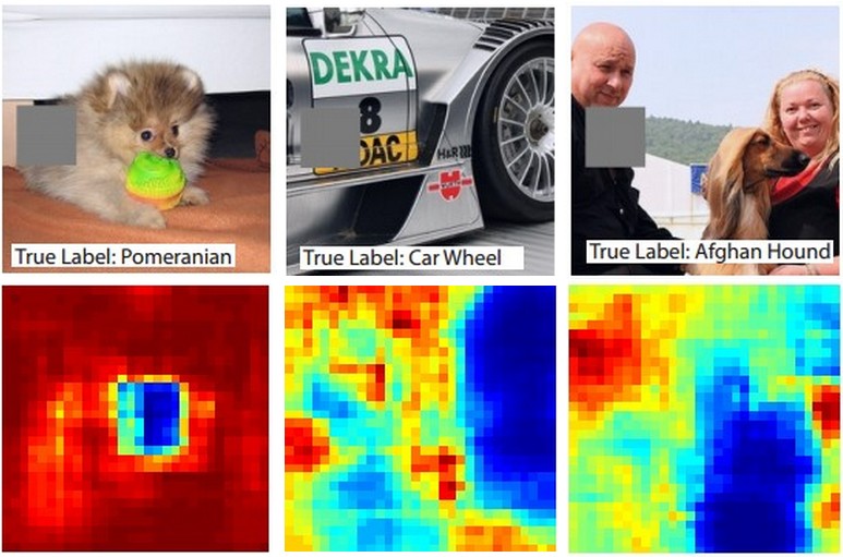
Inspect activations, learned filters, high-response input examples, feature-space embeddings, and the effects of occlusion. Gradient-based visualizations and reconstruction reveal other aspects of a representation, but each method answers a different question and can be misleading when treated as a complete explanation. The reading links also cover adversarial examples, spatial information, attribute-based evaluation, and comparisons with human labelers. [124] [141] [145]


Transfer learning
Reuse a pretrained network as a fixed feature extractor or fine-tune some or all of its layers. Dataset size and similarity to the pretraining domain guide which layers to update and how much regularization to apply. Earlier features are often more general; later ones may be specialized. Use a smaller learning rate for transferred weights, and match the source model’s expected preprocessing. [148] [150]
Recurrent networks
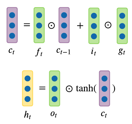
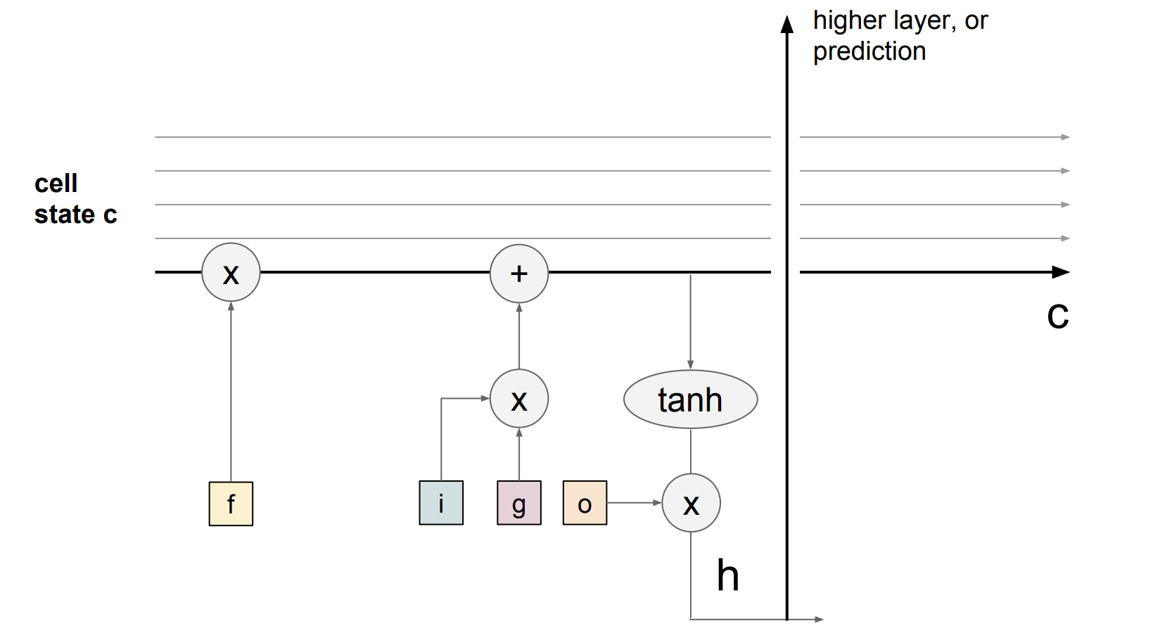
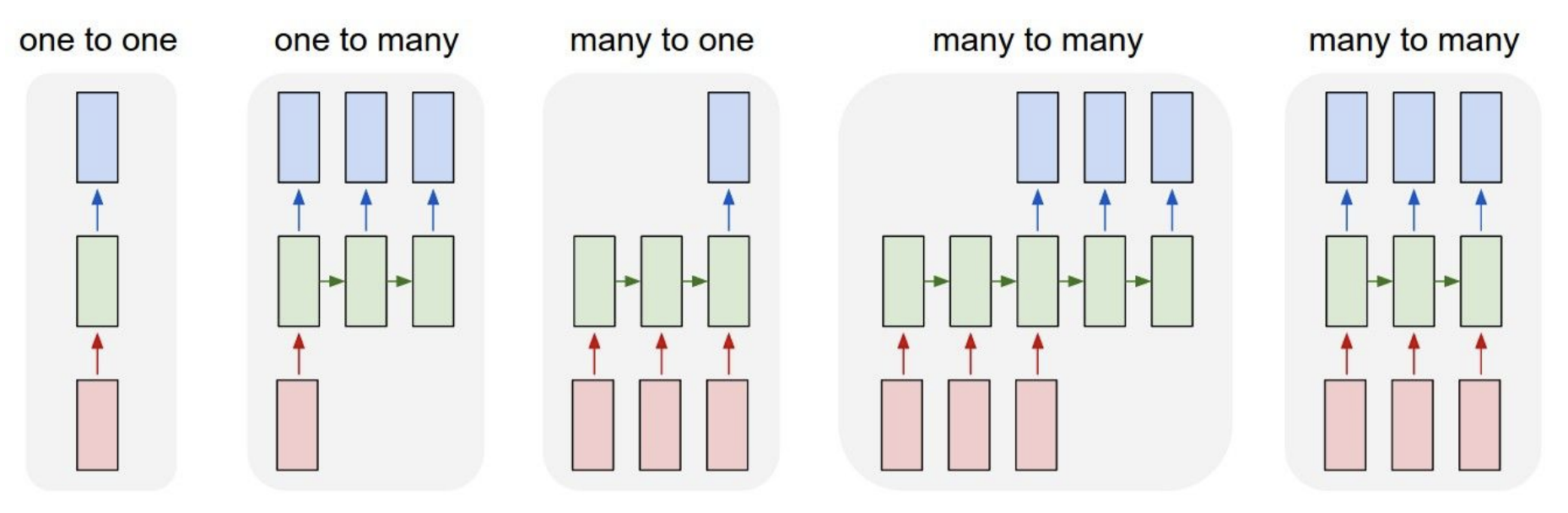
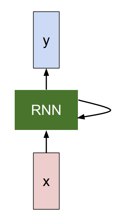
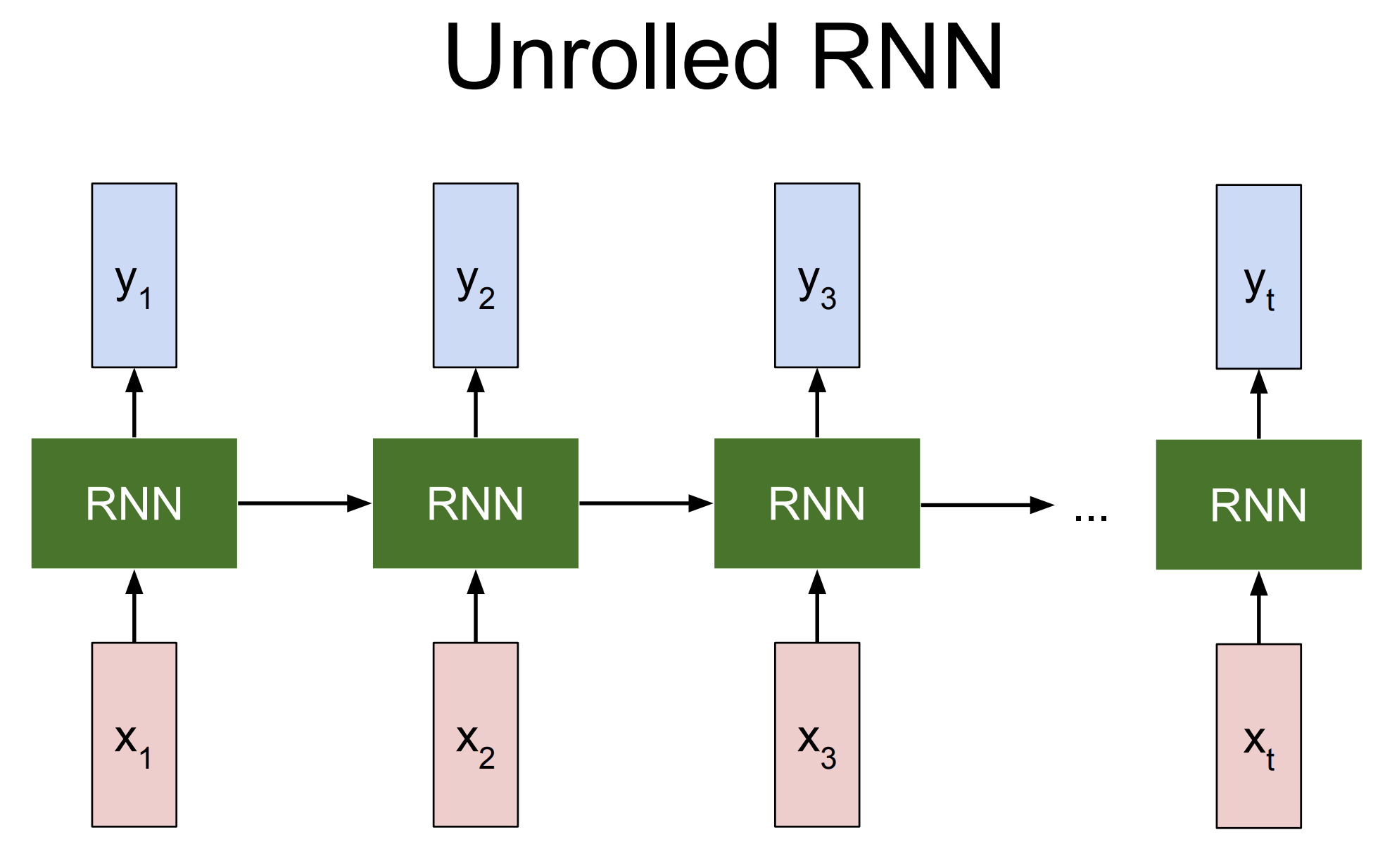
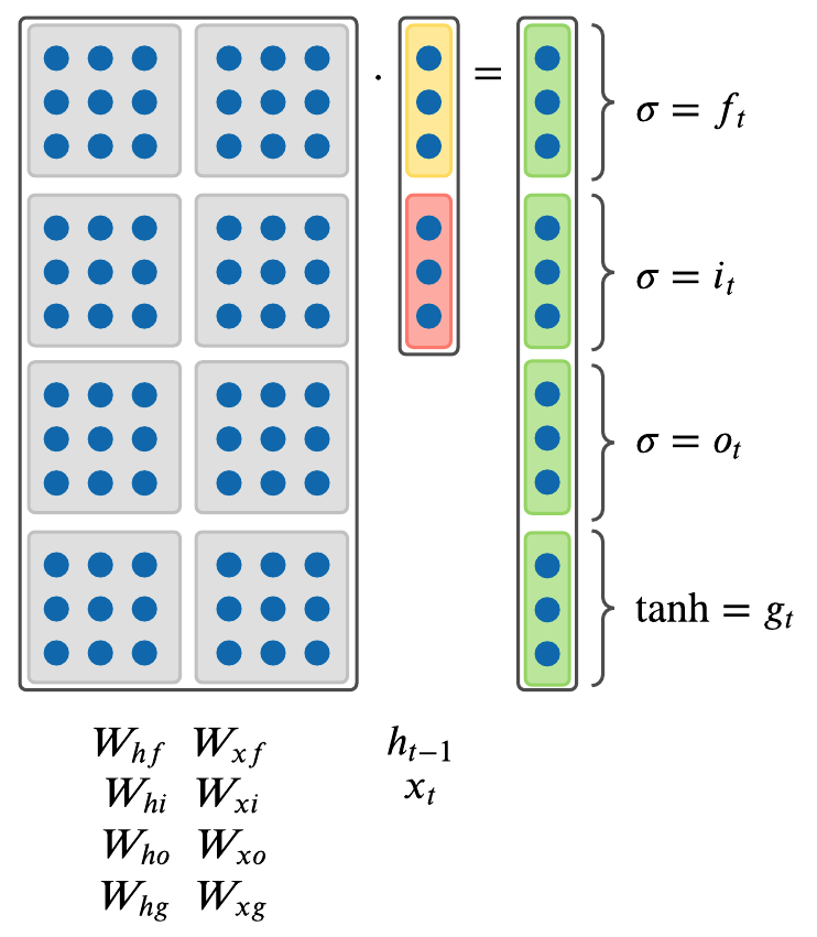
A recurrent state supports sequence inputs and outputs with variable length. Training a character predictor exposes how earlier inputs affect later predictions, and stacked recurrent layers increase depth. Repeated Jacobian products can make gradients vanish or explode. An LSTM adds a cell state with gates controlling retention, updates, and output; this offers a more direct route for information and gradients, without guaranteeing perfect long-term memory.
Equations
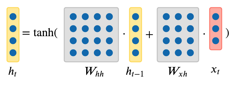
Equation
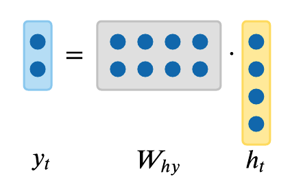
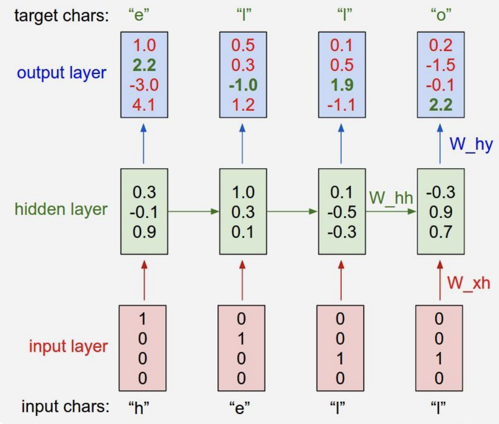
Equations
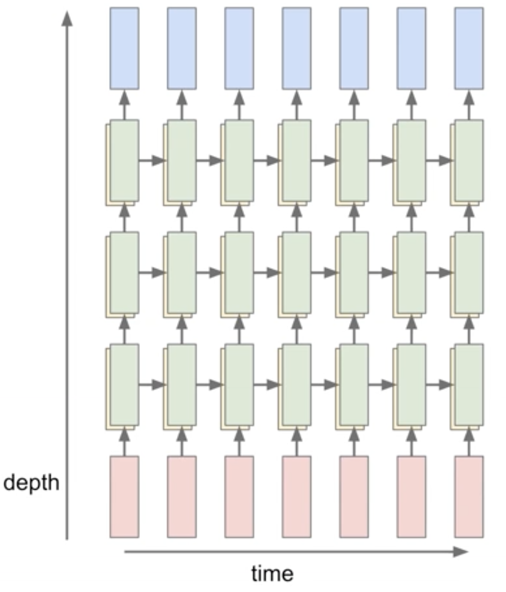
Equations
Equation