Overview
Reading focus: a policy can achieve acceptable single-rollout success while failing to preserve the demonstrator’s alternative actions. This study tests a data-collection intervention for re-queryable demonstrators, with controlled synthetic analysis and simulated truck unloading. The edition keeps all nine figures, three tables, three numbered equations and the complete sampling algorithm.
At a glance
Sliding-window behavior-cloning data usually pair each continuous observation history with only one action sequence. A sufficiently expressive conditional diffusion model can memorize those pairings, collapsing its output at each observation even when the demonstrator is stochastic. Vine sampling instead records several independently queried actions at exactly the same history. At matched numbers of stored training pairs, this improves conditional-distribution matching and downstream search/self-improvement in the tested sparse-data settings. It trades fewer distinct observations and substantially more collection compute for explicit action alternatives; dense-data and hardware benefits are not established.
1 Introduction
Best-of-N search, expert iteration and reinforcement-learning post-training need useful alternatives to choose from, not merely a policy that succeeds once. Ordinary trajectories omit the actions a demonstrator could have taken at each visited state. With continuous high-dimensional observations, exact histories rarely recur, leaving ambiguity between a genuinely multimodal demonstrator and a rapidly changing unimodal function. Repeated queries disambiguate the training target. This requires either resettable environments for closed-loop demonstrators or planners that return actions without changing the world. The paper isolates actions-per-condition k while fixing stored-pair count and training budget, then tests the resulting policies as search and improvement proposals.
2 Related Work
The analysis builds on conditional diffusion memorization results: at training conditions, the ideal denoising solution reproduces the empirical conditional sample distribution. Existing diversity interventions add noise during training/inference or alter latent exploration, while other work deliberately reduces expert entropy for single-rollout success. Here the aim is to preserve expert entropy for downstream search. Multiple labels per condition already appear in language, segmentation, grasping and motion planning; the contribution is a controlled study under the ordinary diffusion objective and a concrete behavior-cloning collection protocol. Prior sparse-data studies motivate the setting without proving that every large robot policy is in the same regime.
3 Problem Formulation
The formulation distinguishes the demonstrator’s conditional distribution, the finite set recorded at one observation and the learned policy distribution. Comparing all three separates a model-fitting problem from a collection-coverage problem.
3.1 Setting
An observation history contains Tₒ timesteps; an action output spans Tₐ future timesteps. Group the dataset by n distinct histories, each with k independently drawn demonstrator action sequences, equivalent to n×k ordinary training pairs. Standard collection uses k=1. Experiments increase k while holding n×k fixed, so explicit action diversity necessarily reduces the number of unique conditioning histories. The policy class is assumed expressive enough to represent the relevant multimodal distributions.
3.2 Study of the trained policy
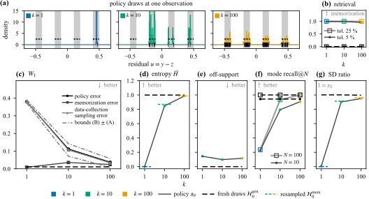
Use Wasserstein-1 distance for distributional error and mode recall@N for whether N draws cover useful modes. Equation 1 bounds policy-to-demonstrator error by model-to-empirical error A plus empirical-to-demonstrator sampling error B; the reverse triangle inequality also gives a lower bound B−A. Thus the policy error lies within A of B. Near exact memorization, A is small, so better fitting alone cannot overcome poor conditional samples: lowering B requires more representative recorded alternatives. This argument is local to training conditions and the memorization regime; a model that generalizes away from training samples can escape the k=1 empirical bottleneck.
Equation 1
| (1) |
4 Analysis
The controlled experiment separates action-mode coverage from generalization across observations. It first holds total sample count at 1,000, then evaluates unseen conditions and larger datasets to identify where repeated queries help.
4.1 Synthetic task
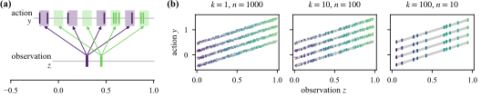
Observations and actions are each 16-dimensional, with one informative observation coordinate z and 15 nuisance coordinates. The first action coordinate y must lie in four equally weighted intervals shifted by z; the other 15 coordinates are independent Gaussian nuisance actions. Widely separated high-dimensional observations mimic sparse visual histories. Random action coordinates make near-exact retrieval across all 16 dimensions strong evidence of memorization rather than merely choosing the same valid task mode. Equation 2 preserves the full distribution, including Gaussian standard deviation 0.3.
Equation 2
| (2) |
4.2 Findings
At 1,000 stored pairs, k=1,10,100 gives 1,000,100,10 distinct conditions. Each policy is queried 1,000 times per condition. All three retrieve training actions frequently at 5%/25% distance tolerances, while fresh demonstrator draws almost never do. Model-to-empirical error stays small; sampling error and policy error fall as k grows. Conditional mode entropy rises from near zero to near one, mode recall and spread improve, and off-support mass changes little. More inference draws barely restore missing modes for k=1.
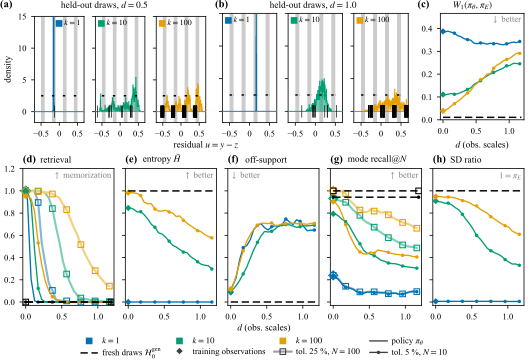
At held-out observations, k>1 retains lower error and better diversity, though its four-mode structure weakens farther from training observations. With 100,000 total pairs, even k=1 generalizes, retrieval approaches zero and its error/diversity largely match larger k. Repeated conditioning is therefore useful here in the sparse-data memorization regime, not a universal requirement for diffusion policies. Entropy only measures mass already within valid support, so the separate off-support metric is essential.
5 Data collection method: vine sampling
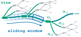
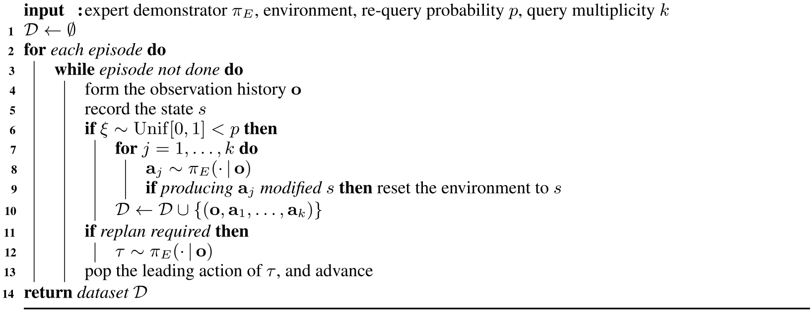
Adapt the vine procedure to collect labels: the demonstrator follows one normal episode, replanning when necessary; independently at each visited timestep, with probability p, re-query k complete candidate action sequences from the identical observation/state. Reset between queries if querying changes the environment, and record only these selected histories with their k labels. Continue the original single trajectory rather than executing all branches. This preserves the episode’s temporal state distribution while exposing counterfactual action choices. Algorithm 1 retains the exact control flow and reset condition.
6 Truck unloading experiments
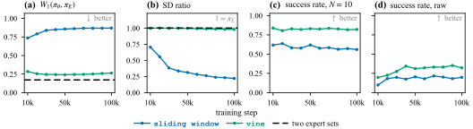
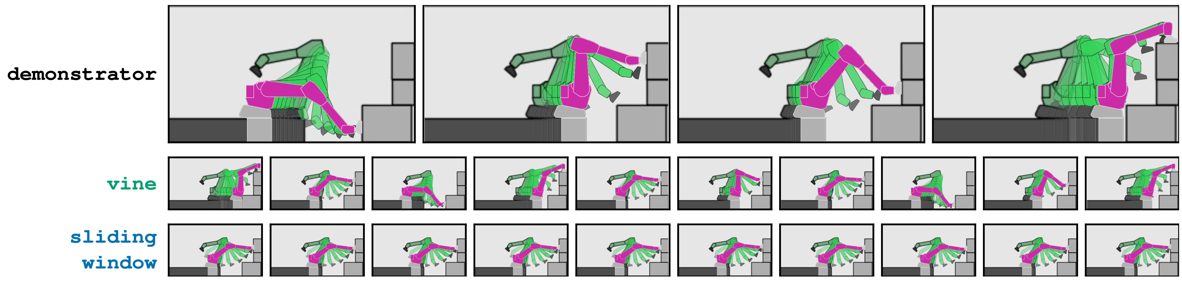
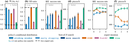
A simulated planar suction robot unloads four boxes before an 80-second timeout. Randomized grasp ordering and motion planning yield alternatives in box choice, grasp face, arm configuration and trajectory. Both methods use the same 2,000 problem instances and 370,000 stored pairs: sliding-window k=1 versus vine k=10,p=0.1, followed by 100,000 training steps. Equal stored-pair count does not equal collection compute. Tests compare raw execution, best-of-N search and expert iteration. Vine better matches the demonstrator’s conditional distribution and improves search success/throughput; later expert iterations retain throughput gains but slightly lose success, plausibly through imperfect distillation and declining diversity.
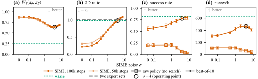
A 20,000-step early-stopped baseline preserves more spread than the 100,000-step sliding-window policy but matches expert choices less well. Raising sliding-window search from N=10 to 100 helps without closing the gap. SIME’s encoder noise approaches vine’s search success but yields lower throughput, more raw-policy failures and worsening later expert iterations; noise can diversify imprecise actions. PostBC widens actions using ensemble uncertainty but only modestly improves distributional coverage and worsens raw success here. These are task-specific comparisons; Figure 5 keeps all uncertainty intervals and raw/search results.
7 Conclusions and limitations
Repeated demonstrator queries preserve alternatives that a memorizing policy cannot infer from one action per unique history. The improvement comes with costs: vine collection takes about 30 times more compute in truck unloading, and p/k were not optimized. The best k for search may differ from the best k for raw execution. All experiments use simulation, including candidate verification inside search and expert iteration. Non-state-changing planners could provide real-world re-queries without resets, but those unexecuted alternatives would not be physically verified. Whether much larger robot models/datasets remain sparse enough to benefit is open.
Acknowledgments
Support is acknowledged from Pickle Robot Company and the Charles Stark Draper Laboratory. Rebecca H. Jiang is a Draper Scholar; part of Shao Yuan Chew Chia’s contribution was made during a Pickle Robot internship.
Appendix A Synthetic Analysis
The appendix specifies the synthetic distribution, training recipe, metric conventions and held-out query construction, then repeats the analysis across four dataset scales. These details qualify the apparent entropy and generalization results.
A.1 Task, datasets and training
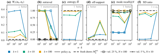
The four residual modes have width 0.1 and centers ±0.15,±0.45, leaving gaps within the overall [−0.5,0.5] range. Twelve policies combine k∈{1,10,100} with total sizes 10²,10³,10⁴,10⁵. Table 1 retains the shared 3.1-million-parameter one-level U-Net, 100-step DDPM, batch 256 and five million training steps, about 13.5 hours per policy on an RTX 4090. This extensive fitting budget matters for the observed memorization; it is not the truck policy’s training recipe.
| Implementation | LeRobot DiffusionPolicy |
|---|---|
| Architecture | 1D convolutional U-Net, one level of width 256 |
| Parameters | 3.1M |
| Diffusion steps | 100 for training and sampling (DDPM) |
| Noise schedule | cosine |
| Prediction target | |
| Optimizer | AdamW, learning rate , weight decay |
| Learning rate schedule | 500-step warmup, then constant |
| Batch size | 256 |
| Training steps | |
| Hardware | NVIDIA RTX 4090, 13.5 h per policy |
A.2 Metrics
Synthetic Wasserstein terms against the expert use its exact cumulative distribution; policy distributions use 1,000 draws. Retrieval searches all stored actions, not just labels at the queried condition. If fewer than 15 draws fall within expert support, conditional entropy is set to zero and that condition stays in the mean. This occurs for 7% of k=1 training conditions and 58% of its held-out queries at 1,000 total pairs, versus none/under 1% for larger k. Reported training means cover up to 128 conditions spaced in z, and reference distributions use the same 1,000-draw budget. This convention prevents selectively dropping failed conditions but affects interpretation of low entropy.
A.3 Held-out conditions
Held-out queries follow random-direction lines from training observations through the 16-dimensional space. Distance d is normalized by the mean pairwise training distance of the k=1,n=1,000 dataset. Use 24 distance bins from 0 to 1.18, with 96 queries per bin and no more than one query from each originating line in a bin. Figure 6 retains representative histograms at d=0.5/1.0 and all metric curves; this constructed probe distribution is not a robot deployment distribution.
A.4 Results against total dataset size
Figure 7 compares all 12 policies over total sample count. At sparse scales, repeated labels improve conditional coverage; at 100,000 pairs, k=1 learns across nearby conditions rather than retrieving individual labels and approaches the other policies on the principal error/diversity measures. This supports a regime-dependent conclusion and does not establish an optimal k for arbitrary architectures or data budgets.
Appendix B Vine Sampling
Algorithm 1 records selected histories along a single demonstrator rollout. Following every queried branch would overrepresent later-time states, so those branches are stored as alternatives and not all executed. Selected conditions occur at probability p across the original temporal distribution. The procedure assumes the expert can plan from any visited state; if partial observability or another restriction prevents that, selection must also test whether that state is queryable. The appendix’s HTML cross-reference to the conditional line is resolved by the preserved original algorithm numbering.
Appendix C Truck Unloading
The truck appendix specifies simulator failures, reward, observations, dataset splits, policy/value architectures, distributional metrics, search and baseline implementations. It exposes both a substantial collection-compute imbalance and a plan-versus-executed-action distinction in the evaluation.
C.1 Task and demonstrator
Drake simulates randomized boxes and a planar robot viewed from the side, removing partial observability as a confound. Observations contain an image plus four joint positions, suction state and a grasped-box flag; two observations condition 32 future actions, each four joint positions plus suction. Excess penetration or excessive tracking error causes failure. Each timestep costs 0.1 reward; failure/timeout costs 100. Failed throughput uses the 80-second timeout duration. The expert shuffles candidate grasps, finds admissible motions with bidirectional RRT, then refines them by trajectory optimization; every visited state is re-queryable.
C.2 Problem instances and datasets
Training uses instances 0–1,999; expert iteration uses 2,000–6,999; other tests share 600 separate instances. The expert achieves 95.8% success and 766 pieces/hour on that test set. Failed demonstration episodes remain in both datasets: successful counts are 1,899 sliding-window and 1,878 vine episodes. Vine stores returned plans; sliding-window stores executed motion, which includes controller tracking error. Distributional evaluation also compares against re-queried plans, favoring the same action representation used for vine training; this is an explicit measurement distinction. Collection takes 55 versus 1.8 seconds per episode on a 96-core machine.
C.3 Policy and value networks
Tables 2/3 preserve the full architectures and optimization settings. Both policies share the CNN U-Net with widths 256/512/1024, from-scratch ResNet-18 encoder,100-step DDPM, batch 2,048,100,000 steps and exponential moving-average weights; only data differ. Policy training takes about 8 hours on two H100 GPUs. The shared initial value function uses one image plus six state coordinates, a ResNet/MLP architecture and tanh output, trained 100,000 steps with batch 1,024 and Adam learning rate 2×10⁻³, about 4.9 hours on one H100. PostBC changes training targets rather than this policy architecture.
| Architecture | CNN-based U-Net of Chi et al. [10], channels |
|---|---|
| Image encoder | ResNet-18 trained from scratch, GroupNorm, spatial softmax |
| Diffusion steps | 100 for training and sampling (DDPM) |
| Noise schedule | cosine |
| Optimizer | AdamW, learning rate (constant), weight decay |
| Batch size | 2048 |
| Training steps | 100,000 |
| EMA of weights | yes |
| Hardware | two NVIDIA H100 GPUs, about 8 h per policy |
C.4 Metrics
Select 576 states along expert test episodes with probability 0.005/timestep, then retain 507 where all 200 expert queries return plans. Split those queries into 100-action estimate/reference sets, and compare 100 draws from each policy. Equation 3 defines RMS trajectory distance after scaling each coordinate by expert standard deviation across all evaluation states/timesteps. Policy error is Wasserstein-1 under that distance; spread is RMS distance from the mean, normalized by expert spread. Filtering to fully plannable states limits the evaluated distribution. Error/spread/throughput intervals bootstrap problem instances 1,000 times, preserving within-instance dependence; success uses equal-tailed Beta(1+successes,1+failures) posterior intervals. All are 95%, but they are not the same interval construction.
Equation 3
| (3) |
C.5 Best-of- N search and expert iteration
Best-of-N simulates each candidate’s first 20 timesteps, rejects failures, ranks survivors by simulated reward plus learned terminal value and executes the best; all-failed candidates end the episode. Planning time does not advance simulation time, so pieces/hour excludes search latency. Expert iteration uses best-of 100 to collect 1,000 fresh instances per iteration, then fine-tunes policy and value for 10,000 steps with older data weighted 0.8ʲ. Every method uses ordinary sliding-window collection during these later iterations: only initialization benefits from vine. Value networks begin shared but diverge under fine-tuning. Iteration curves report the 1,000 collection instances themselves, not a separately evaluated policy test set; iteration 0 is base-policy best-of 100 on new instances.
C.6 SIME and PostBC
SIME adds one image-encoder noise sample per action draw, linearly annealed to zero through denoising; scaleσ=4 is chosen from the sweep to approximately match expert spread and minimize policy error. Its absolute amplitude uses encoder-output RMS standard deviation over 576 states. During expert iteration, that base-policy noise level remains fixed. PostBC trains 10 bootstrapped conditional-mean regressors, each using the image encoder plus three 512-unit MLP layers for 6,000 steps at batch 256. Their prediction covariance spans the full 32×5 action sequence and supplies fresh Gaussian target noise with α=1. Ensemble size/α follow defaults without tuning, with fewer ensemble-training epochs because this dataset is larger.
C.7 Results against training step
Figure 9 preserves checkpoints every 10,000 training steps. Sliding-window spread falls while its policy error remains high; vine maintains broader, better-matched conditionals and stronger best-of 10 success. Both raw-policy curves remain much lower than search-assisted success. The 20,000-step early-stopping comparison is selected for similar raw success/throughput to the fully trained sliding-window policy, not as a universal optimum.