Reading guide
This edition covers all 22 pages, the complete appendix, twelve figures with every subpanel, ten numbered tables and both exact prompt payloads. Mohamed Elmoghany, Kehan Li and Ruoqu Chen contributed equally. Human capture is real-world; the reported robot policy table uses simulated reference tracking. The project separately shows selected physical squeegee rollouts. Reasoning-output validity, image quality and physical task completion are distinct quantities.
At a glance
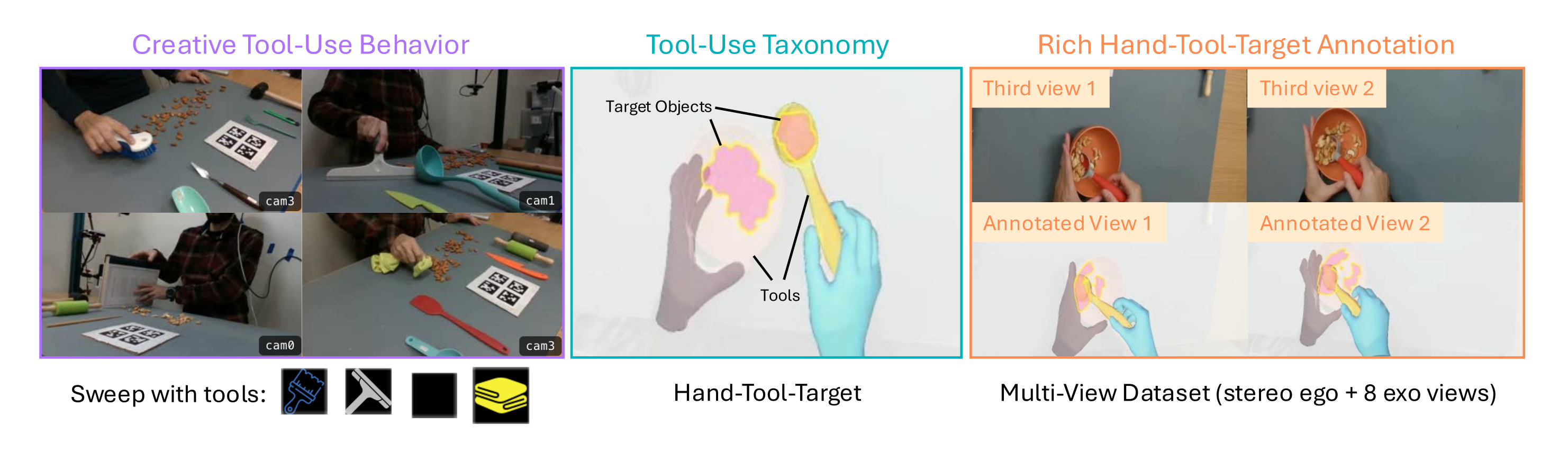
ToolDex records creative tabletop hand–tool–target interactions with stereo ego and eight exocentric RGB-D cameras. Its reported 10,853 trials cover sixty task combinations and 168 variants. Benchmarks study sparse-view image reconstruction, VLM tool selection/pointing/trajectory outputs and human-to-robot policy transfer. The suite supplies useful diagnostics, while selected tools, simulated reference success and repaired image appeal do not by themselves establish robust physical creative tool use.
1 Introduction
Repurposing everyday objects requires contact geometry, material properties and task constraints beyond recognizing canonical tool names. The dataset explicitly separates hands, actuated tools and affected targets, including deformable/granular objects. Shared scenes support several benchmarks, but results at one level do not automatically transfer to the others. The comparison with TACO concerns role/annotation design rather than an assertion that earlier datasets contain no target objects.
2 Related Work
Prior hand/object datasets, physical reasoning suites and robot tool-use methods cover complementary settings. Table 1 preserves the authors’ inventory comparison, including its explanation that dashes in prior target columns denote combined inventories. ToolDex’s particular contribution is explicit hand–tool–target data and several aligned diagnostics; broad claims that no competing multi-camera dataset could support held-out views are not demonstrated by this comparison alone.
3 The ToolDex Dataset
The collection formalizes target-centric physical interactions and records both tool motion and human hand motion. These representations enable retargeting research without guaranteeing that every robot can reproduce a human trajectory.

Accessible table, original values and citations
| Dataset | #Tools | #Target Obj. | #Actions | #Frames | #Trials | Ego/Exo | Channels | Hand Pose | Obj. Pose | Seg. Mask |
| TACO Liu et al. (2024) | 20 | – | 15 | 5.2M | 2.5K | 1 / 12 | RGB (Ego RGB-D) | ✓ | ✓ | ✓ |
| OakInk2 Zhan et al. (2024) | 75 | – | 60 primitives | 4.01M | 2.8K | 1 / 3 | RGB | ✓ | ✓ | ✓ |
| HOT3D Banerjee et al. (2025) | 33 | – | – | 3.7M | 2.8K | 2–3 / 0 | RGB + mono | ✓ | ✓ | ✓ |
| GigaHands Fu et al. (2025) | 417 | – | 1467 | 183M | 13.9K | 0 / 51 | RGB | ✓ | ✓ | ✓ |
| TOOLDEX | 45 | 23 | 16 | 58.3M | 10.8K | 1 / 8 | RGB-D | ✓ | ✓ | ✓ |
3.1 Problem Formulation
Tools mediate changes to targets, while support objects constrain the interaction without being the actuated tool. A goal-conditioned MDP describes complete scene state, hierarchical tool/agent actions, physical transitions and language/terminal-observation goals. The dataset records observed trajectories, not direct access to the full physical transition function or every material variable.
Target-centric tool manipulation.
The hand controls a tool whose contact changes a separate target. This role decomposition matters for annotation and evaluation; object names alone do not determine affordances. Supports such as containers or work surfaces may influence success even when they are not actuated.
Tool manipulation as a goal-conditioned MDP.
Each trial pairs a state/action trajectory with a language goal and a successful terminal observation. The full original MDP, state/action/goal spaces and trajectory definitions remain selectable. The two action levels are a modeling abstraction, not a measured two-level causal dynamics model learned in these experiments.
Original mathematical definition and evaluation protocol
We formalize a tool-manipulation trial as a goal-conditioned Markov decision process . The state is the configuration of all participants of the scene—tool, target, support, and agent—at time . The action is decomposed into two levels: a tool action that determines how the tool moves and, through contact, how the target’s state changes; and an agent action that determines how the agent’s manipulator moves and thereby controls the tool. The transition captures the physics of the interaction. The goal is the desired terminal state of the target object, specified per trial in two complementary ways: a natural-language description , and a terminal-observation from a successful demonstration. A trial is a trajectory paired with language goal , and ToolDex is a collection of pairs.
3.2 Dataset Properties and Statistics
The source reports 10,853 trials, 60 task combinations, 168 variants, 45 tool objects, 23 support objects, 16 deformable object types and 16 actions. Table 1 instead labels 23 as target objects; category/instance/support wording is not fully reconciled. Likewise 58.3 M table frames and 6,158,809 annotated frames use different unexplained counting conventions. Notes retain those labels rather than silently treating them as one statistic.
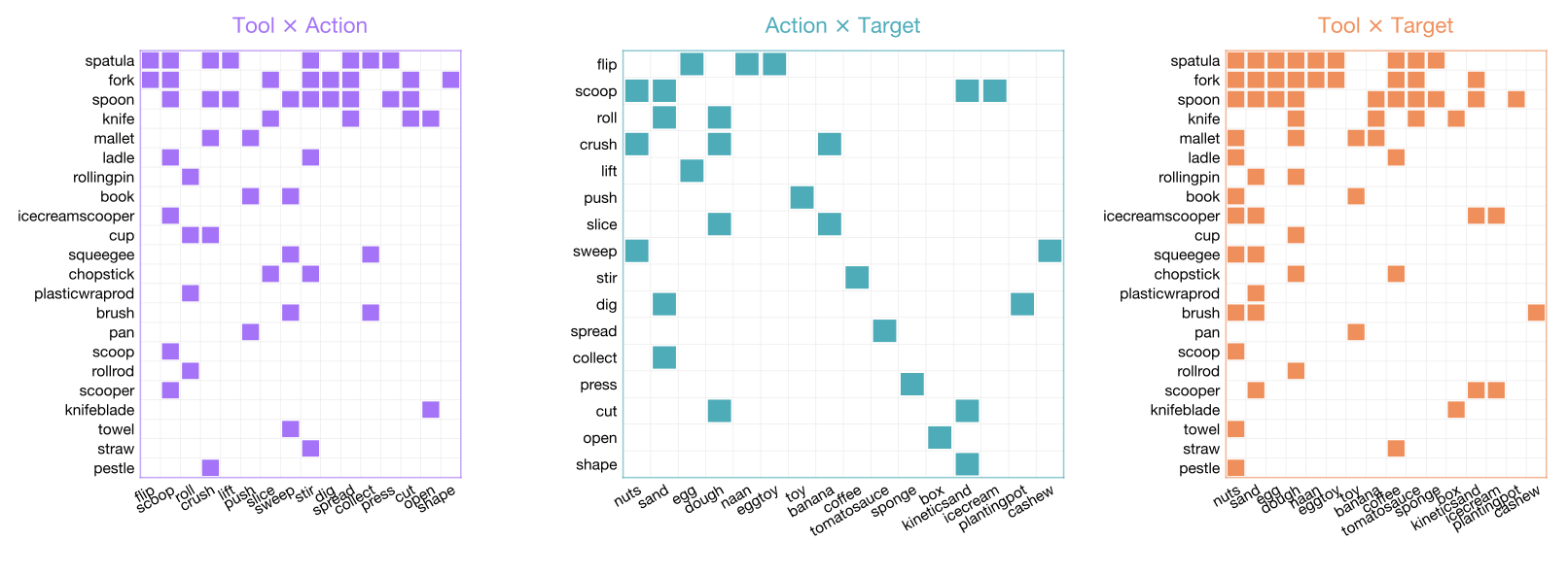
Diversity of tools, target objects, and actions.
Tool shapes and materials vary across canonical and repurposed objects, with 4–5 distractors and changing starts. Sixty task combinations receive nominal one-hour collection blocks. Coverage heatmaps show observed pairwise relations, not all possible triples or equal difficulty across them. The project’s sixty-row task inventory sums to 10,853 trials, but its category summary fields and histogram keys do not fully clarify the manuscript’s inventory terminology.
Zero-shot and compositional generalization.
The authors define withheld tool, target or action splits and held-out combinations of individually seen components. These are useful proposed generalization settings. The reported six-task policy table does not supply results for each of these split families, so the existence of a split is not evidence of demonstrated zero-shot robot transfer.
Multi-view capture of 3D interaction.
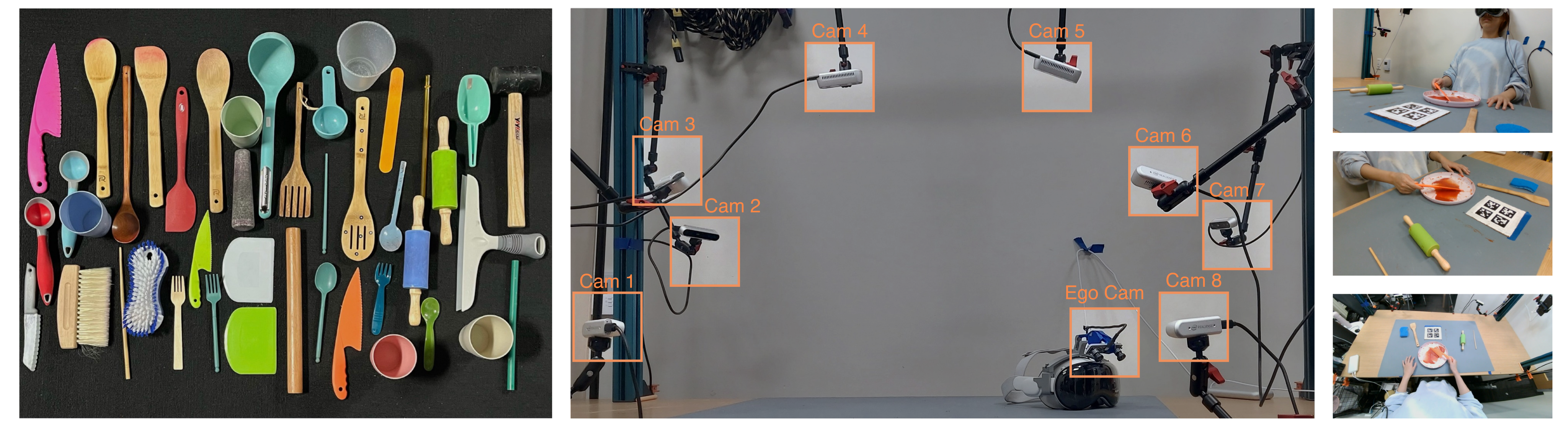
Eight calibrated exocentric streams record 1280×720 RGB-D at 30 Hz, with two extra ego RGB views from the headset-mounted ZED Mini. Mean 567.58 frames/18.92 seconds is consistent with 30 Hz. Synchronization and depth enable multi-view annotation, though occlusions/contact remain error sources. Multiple image streams should not be confused with unique interaction timesteps.
Original mathematical definition and evaluation protocol
We capture each interaction with high fidelity to recover the 3D state of the tool, target, and hand, which together provide the inputs required to learn the interaction function T defined in Section 3.1. Each trial records eight calibrated exocentric Intel RealSense RGB-D streams at resolution and 30 Hz, together with a stereo egocentric stream from a ZED Mini stereo camera mounted on an Apple Vision Pro headset worn by the demonstrator. Depth observations from each exocentric viewpoint enable 3D reconstruction of state changes, while synchronized multi-view videos capture non-rigid phenomena such as dough deformation and granular flow. We provide per-frame multi-view segmentation masks for the target object, and tool and hand. Each trial lasts an average of 18.92 seconds and contains 567.58 frames.
Embodiment-agnostic data representation and collection.
Tool 6-DoF trajectories describe intended physical interaction; MANO/wrist trajectories support embodiment-specific retargeting. Transfer still requires reachable motions and compatible contact/control. The paper’s 60 hours and 10,853 trials imply about 181 trials/hour, unlike its separate reported 60-trials/hour throughput; an alternate collection/processing denominator is not stated. Annotated 30 Hz timesteps represent about 57 hours, so active trial time and session time should remain distinct.
4 Data Collection
A single calibrated studio rig and scripted task protocol produce synchronized views, then offline automatic annotation with manual verification/corrections. Data diversity is substantial within tabletop capture, while demonstrator/site/background diversity and annotation accuracy distributions are not fully quantified.
4.1 Task and Object Curation
Sixteen everyday scenarios expand through alternative tools to sixty combinations. Instructions describe both tool motion and target effect; clutter and poses vary. Demonstration collection follows predetermined procedures, so 'creative' describes curated substitution/repurposing rather than unconstrained discovery of novel strategies during every trial.
Original mathematical definition and evaluation protocol
Each task combination is a (tool, action, target) triplet specifying a set of demonstrations. We curated the task combinations in two stages. We first enumerated 16 everyday tabletop tool-use scenarios drawn from cooking, food preparation, child play, and household activities, each defined by an action verb and a default tool–target pair. We then expanded each scenario along the actiontool axis. For each action, we explicitly enumerated the alternative tools a human might creatively substitute when the canonical tool is unavailable. We select tool, target, and support objects to span diverse geometries, material properties, covering rigid, granular, and deformable objects. Within each task combination, we vary the initial pose of the tool and target object on the work surface, and additionally place 4-5 tool objects as distractor objects in the scene to match the cluttered tabletop conditions of real deployments and require visual grounding of the correct tool when conditioned on language. Each task combination is paired with a natural-language instruction that specifies both the tool motion (e.g., “swing the spatula laterally under the egg, then lift”) and the intended effect on the target (“flip the egg so its underside faces up”).
4.2 Hardware Setup
Eight RealSense 435 RGB-D cameras surround the workspace; a ZED Mini mounts on Vision Pro. AprilTag calibration and bundle adjustment recover rig parameters, while a scanner provides textured tool meshes. Exo streams are software synchronized. These extra sensors/meshes enable annotation and reconstruction; they are not a demonstration of equally accurate sparse uncalibrated onboard perception.
Original mathematical definition and evaluation protocol
Our capture rig (Figure 3) consists of 8 Intel RealSense 435 RGB-D cameras and an Apple Vision Pro headset fitted with a Stereolabs ZED Mini stereo camera. The 8 RGB-D cameras are mounted on a Vention extruded-aluminum frame surrounding the work surface, in positions designed to maximize joint coverage of the work volume while preserving sufficient view overlap for multi-view triangulation, 6-DoF object pose estimation, and 4D scene reconstruction. RGB and depth streams are recorded at resolution and 30 Hz; streams across the 8 cameras are synchronized in software. We calibrate the cameras using an April Tag followed by multi-view bundle adjustment to obtain rig-relative camera parameters. The ZED Mini, mounted on the Vision Pro, provides two additional stereo RGB egocentric streams. To support 6-DoF tool pose estimation, we scan each tool with a Shining3D scanner to obtain a high-resolution textured mesh. The sparse 8 camera setup overcomes occlusion and enables photo-realistic 3D and 4D scene reconstruction.
4.3 Data Collection and Annotation
SAM2 propagates masks from DINOv2-related initialization; FoundationPose estimates per-view tool poses using scans/masks, then confidence fusion and temporal bundle adjustment combine them. WiLoR hand estimates are aligned to depth/triangulated keypoints for metric MANO trajectories. Joint reprojection/depth/tool/contact losses refine them; human annotators correct failures. The manuscript promises detailed annotation hyperparameters/ablations in the appendix, but the supplied appendix mainly covers benchmark pipelines and does not provide those full numerical annotation ablations. No unreported accuracy guarantee is inferred.
5 Creative Physical Tool-Use Benchmarks
Reconstruction, VLM reasoning and policy learning use different subsets, sensors and success measures. Their common source dataset does not make their scores interchangeable or establish a causal progression from better VLM output to better robot control.
5.1 Novel-View Gaussian Splatting for Sparse-View Tooluse: Static and Dynamic
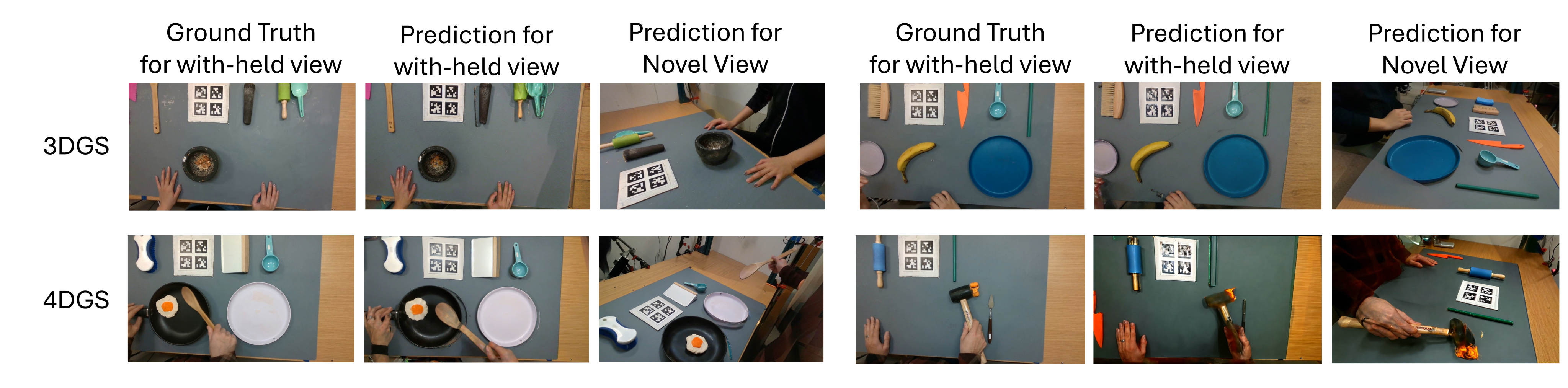
Static InstantSplat and independent per-timestep InstantSplat-4D fields are followed by rendered-view diffusion repair. Held-out cam 6 full-reference fidelity and eight-camera-run reference-free appearance are evaluated in separate reconstructions. The latter is image appeal, not geometric ground truth or temporal consistency.
Experiment setup.
Each scene has a seven-view training run with cam 6 withheld and a separate all-eight-view run. Main static/dynamic results use three scenes each, not the full dataset. Per-timestep independent fields should not be mistaken for a single temporally coupled4D dynamics model.
Original mathematical definition and evaluation protocol
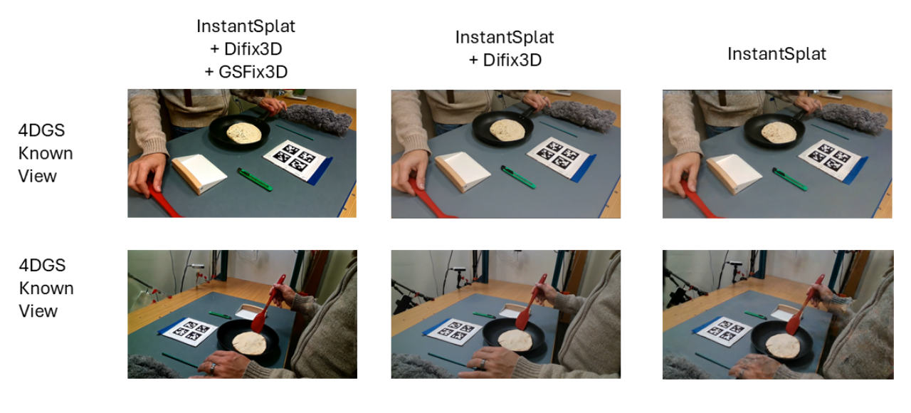
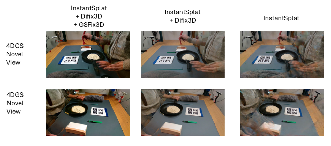
We benchmark sparse-view novel-view synthesis on 8-camera calibrated capture in two regimes: (i) static 3DGS using InstantSplat (Fan et al., 2024) (IS) as a backbone (ii) dynamic 4DGS training InstantSplat on -frame sequences applied per-timestep, denoted IS-4D. Each scene is reconstructed twice (once with 8 cameras and once with cam6 dropped for ground truth comparison). We add a second stage single-step diffusion to the pipeline utilizing GSFix3D (Yin et al., 2026) and Difix3D (Wu et al., 2025) to enhance reconstruction and decrease noise.
Method evaluation.
MASt3R seeds InstantSplat; stage 1 uses 1000 photometric iterations without depth/distortion/normal penalties. Difix3D repairs rendered views; GSFix3D is added for the dynamic variant. Image-space repair may improve visual plausibility without improving underlying3D geometry. Original formulas and all exact metric tables remain.
Reconstruction results.
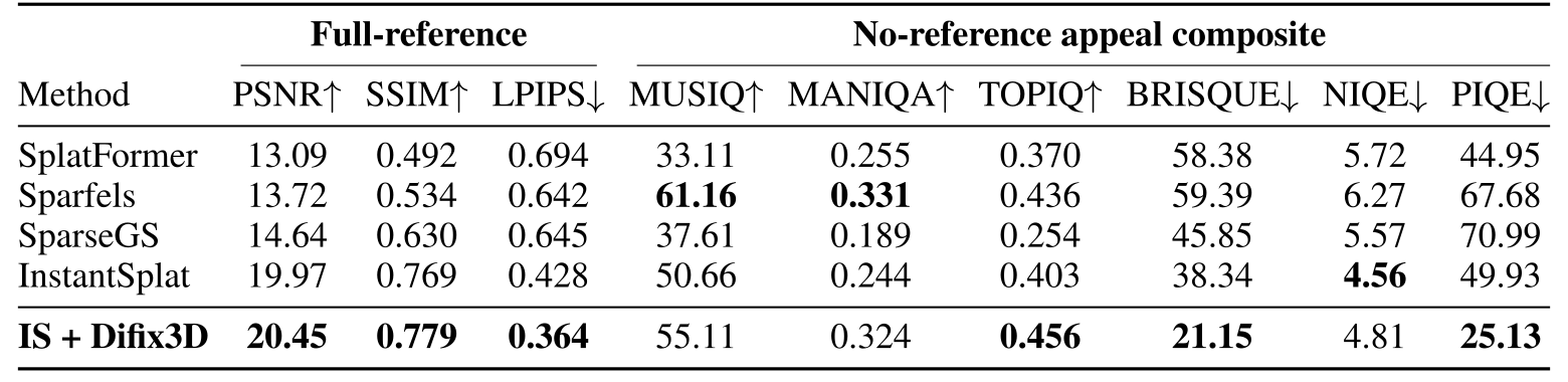
Static Difix raises held-out PSNR 19.97→20.45 and MUSIQ 50.66→55.11, while Sparfels still has higher MUSIQ 61.16. Dynamic full repair raises MUSIQ 51.00→69.92 but lowers held-out PSNR 19.60→15.97. The reference-free and full-reference columns come from different training-view protocols; the dissociation is not paired scoring of an identical trained model/render. A higher appearance score does not establish more faithful reconstruction.
Original mathematical definition and evaluation protocol
Table 2 summarizes both regimes. PSNR (in dB; higher = closer pixel-by-pixel to the held-out cam6 ground truth) measures photometric fidelity, while MUSIQ (on a 0–100 scale; higher = better learned-perceptual appeal) judges visual quality without any reference. Static: IS + Difix3D reaches 20.45 PSNR / 55.11 MUSIQ, beating InstantSplat alone by dB and SplatFormer (Chen et al., 2025) by dB. Dynamic: IS-4D + Difix3D + GSFix3D reaches 69.92 MUSIQ ( over IS-4D) while lowering PSNR by 3.6 dB – the photometric-vs-perceptual trade-off (Wu et al., 2025) is now measurable on held-out 4D. Both findings are made quantifiable only by our dataset’s calibrated 8-camera capture, which uniquely supports a held-out camera view test on tool-use scenes that competing tabletop datasets cannot reproduce. Without it, neither the static held-out gap nor the 4D photometric-vs-perceptual dissociation can be measured.

5.2 Benchmarking VLMs’ Physical Tool-use Capabilities
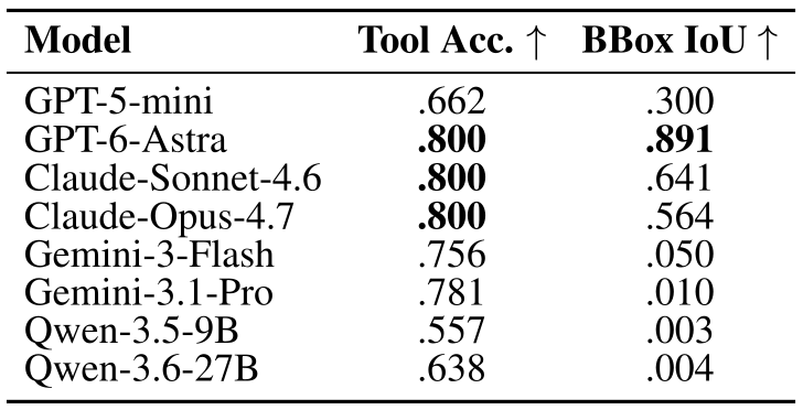
Tool selection credits a prediction list if any item matches the demonstrated tool; it does not measure precision of every suggested alternative. Grounding IoU is computed only for semantically matched tool predictions, so it is conditional rather than end-to-end accuracy. Main text cites 180 verified trajectories/32 variants, while the behavioral table reports 160; the exclusion relation is not explained. Trajectory evaluation-success means evaluable outputs, not a physical execution success rate.
Tool selection and spatial grounding results.
Three models tie at.800 demonstrated-tool hit rate. GPT-6-Astra has.891 conditional box IoU, while several models have high selection hits and nearly zero IoU. Because false positives in tool lists are not fully penalized and alternative tools lack complete human-validated acceptable sets, this cannot be read as an 80% precise assessment of all plausible tools.
Behavioral planning results.
GPT-6-Astra has 89.4% evaluable outputs on the 160-case table. Gemini Robotics ER has lower conditional trajectory errors but 77.5% evaluability; Qwen has 37.5%. Means over successful parsing/evaluation condition on different output subsets, so their ranking alone does not establish better overall physical planning. Pixel errors are substantial and no robotic execution tests these predicted2D paths.
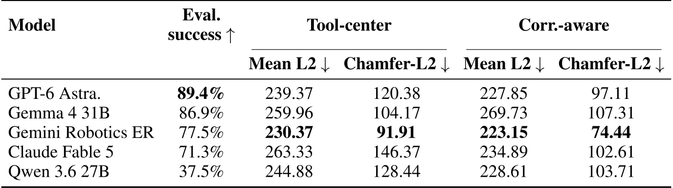
Accessible table, original values and citations
| Model |
|
Tool-center | Corr.-aware | ||||
| Mean L2 | Chamfer-L2 | Mean L2 | Chamfer-L2 | ||||
| GPT-6 Astra. | 89.4% | 239.37 | 120.38 | 227.85 | 97.11 | ||
| Gemma 4 31B | 86.9% | 259.96 | 104.17 | 269.73 | 107.31 | ||
| Gemini Robotics ER | 77.5% | 230.37 | 91.91 | 223.15 | 74.44 | ||
| Claude Fable 5 | 71.3% | 263.33 | 146.37 | 234.89 | 102.61 | ||
| Qwen 3.6 27B | 37.5% | 244.88 | 128.44 | 228.61 | 103.71 | ||
Qualitative results.
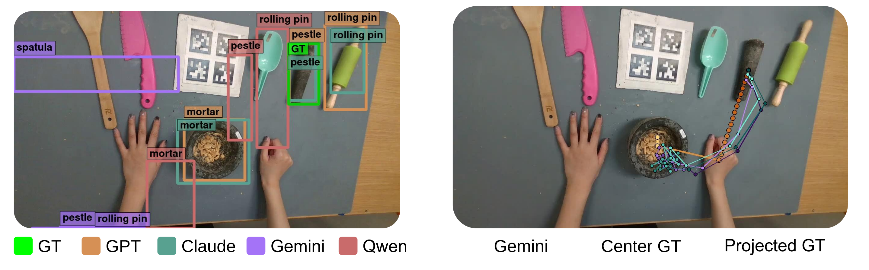
Selected boxes and trajectories illustrate alternate tools and incomplete long-horizon behavior. A grinding task can require repeated contact that a coarse path omits. These examples show plausible high-level geometry, not verified force control or successful material transformation.
5.3 Robot Physical Tool-Use from Human Demonstrations
The policy comparison transfers retargeted human references to dexterous robots in simulation. Kinematic replay and BC are compared with residual interaction-aware RL. Different robot embodiments/action spaces are used for ManipTrans and Dex-X, so their gap is not a fully controlled algorithm-only comparison.
Results.
The six-task means are 14.0% kinematic replay, 4.6% BC, 40.5% ManipTrans and 55.1% Dex-X. Scooper/nuts is a counterexample to uniform dominance: 45.3% ManipTrans versus 31.3% Dex-X. Appendix success is completion of the reference interaction without tracking/stability violations, not an independently measured creative task outcome. The source gives the retained per-task uncertainties but does not report a training-seed count.
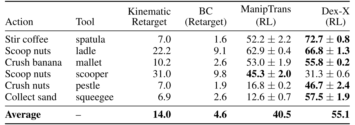
Accessible table, original values and citations
| Action | Tool | Kinematic Retarget | BC (Retarget) | ManipTrans (RL) | Dex-X (RL) |
| Stir coffee | spatula | 7.0 | 1.6 | 52.2 2.2 | 72.7 0.8 |
| Scoop nuts | ladle | 22.2 | 9.1 | 62.9 0.4 | 66.8 1.3 |
| Crush banana | mallet | 10.2 | 2.6 | 53.0 1.9 | 55.8 0.2 |
| Scoop nuts | scooper | 31.0 | 9.8 | 45.3 2.0 | 31.3 0.6 |
| Crush nuts | pestle | 7.0 | 1.9 | 16.8 0.2 | 46.7 2.4 |
| Collect sand | squeegee | 6.9 | 2.6 | 12.6 0.7 | 57.5 1.9 |
| Average | – | 14.0 | 4.6 | 40.5 | 55.1 |
Findings.
Contact, tool geometry and human/robot mismatch make transfer difficult. The table supports interaction-aware adaptation under the tested simulator/tracking protocol. The project separately shows a Sharpa/Franka squeegee deployment, without a hardware trial denominator for all six tasks; neither establishes arbitrary tool/target generalization.
6 Conclusion
ToolDex combines rich real human capture with diagnostic reconstruction/reasoning and simulated policy benchmarks. Consent and a research/non-commercial release are stated in the manuscript. The scope remains curated indoor tabletop activity; materials, sites, embodiments and acceptable-tool labels are incomplete.
AI use statement
The authors disclose AI assistance with literature, statistics, code, writing and experimental design, and state they verified results/artifacts and retain responsibility.
Original data, reconstruction and policy visualizations
All 39 unique original project clips remain byte-unchanged: annotations/multi-view capture, static/dynamic reconstructions and comparisons, two selected real-robot squeegee deployments, a simulation policy and all 17 published human/tool trajectory examples. Original trajectory posters and generated first-frame previews accompany them. The primary summary and sixty-row inventory support 10,853 trials but do not resolve every manuscript count/label. Interactive full-dataset browsing remains linked externally; selected clips add no independent quantitative trials.
Appendix A Appendix
The full appendix preserves reconstruction protocols/tables, all additional views, both exact VLM prompts, boxes/trajectories, retargeting images and policy evaluation/training details.
A.1 Novel-View Gaussian Splatting for Sparse-View Tooluse: Static and Dynamic
Additional reconstructions distinguish held-out cameras from training-view reconstruction. Three-scene static/dynamic tables and twenty-scene observed-view expansion are separate experiments; no single metric summarizes all of them.
Experiment Setup.
The seven-camera run reserves cam 6 for PSNR/SSIM/LPIPS; the all-eight-camera run supplies reference-free novel-view scores. Static comparison uses three named scenes. Initialization differs by baseline, so results compare whole pipelines rather than one isolated regularizer. Multi-view benchmark support follows calibration, but exclusivity over all earlier datasets is not established here.
Original mathematical definition and evaluation protocol
We benchmark sparse-view novel-view synthesis in two regimes that share a single calibrated capture: static 3DGS on a per-scene image, and dynamic 4DGS on a per-scene sequence. In both cases we use the same 8 calibrated RealSense cameras and the same held-out cam6 Protocol B – each scene is reconstructed twice: an 8-cam run that uses all eight cameras for training and a cam6-dropped run that uses cam for training and reserves cam6 for held-out evaluation. From the cam6-dropped run we score the predicted cam6 image (or render across time at cam6’s pose, in 4D) against the captured ground truth with full-reference PSNR, SSIM (Wang et al., 2004), and LPIPS (Zhang et al., 2018). From the 8-cam run we score the rendered novel-view tour without a reference using the appeal-composite metrics MUSIQ (Ke et al., 2021), MANIQA (Yang et al., 2022b), TOPIQ (Chen et al., 2024), BRISQUE (Mittal et al., 2012), NIQE (Mittal et al., 2013), and PIQE (N et al., 2015). Baselines use their native initialization: SparseGS reads the COLMAP (Schönberger et al., 2016, Schönberger & Frahm, 2016) sparse reconstruction, while Sparfels, SplatFormer (applied to our InstantSplat model), and InstantSplat are seeded from MASt3R (Leroy et al., 2024). We use InstantSplat (Fan et al., 2024) as our main backbone; in the dynamic regime we apply InstantSplat across the timesteps, which we refer to as InstantSplat-4D.
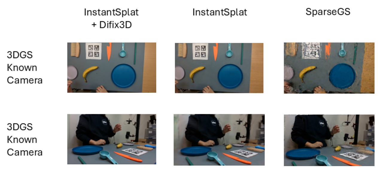
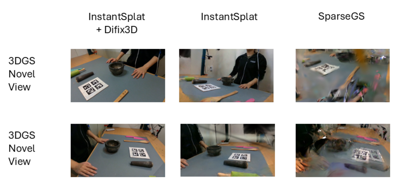
Method.
Each timestep gets its own Gaussian field and MASt3R initialization; rendered-view repair then modifies appearance. The text says repair is tuned to tool-use rendering without complete numerical tuning/training settings here. Omitting regularizers is a chosen setting; no retained ablation table quantifies every omitted penalty.
Original mathematical definition and evaluation protocol
We propose a two-stage sparse-view recipe specifically engineered for the failure modes of unposed tabletop tool-use reconstruction, taking the seven (or eight) training views of our calibrated capture as input – and, in the dynamic case, applied across timesteps. Stage 1 – reconstruction. We obtain a geometry-aware initialization from a MASt3R (Leroy et al., 2024) cross-view dense point prior and train the joint pose-and-Gaussian optimizer of InstantSplat (Fan et al., 2024) for 1k iterations under a clean photometric loss; we deliberately omit every reconstruction-time regularizer (depth, distortion, normals) that we found to leave held-out PSNR flat or harm SSIM/LPIPS in our setting. For 4DGS we instantiate an independent Gaussian field at each timestep using the same Stage-1 design, with the MASt3R prior recomputed per timestep. Stage 2 – rendered-view repair. Rather than expending optimizer budget on 3D losses that do not address the dominant sparse-cam failure mode, we move the heavy lifting to the rendered-view level where ghosting and missing high-frequency detail actually live. For 3DGS we apply a single-step diffusion utilizing Difix3D (Wu et al., 2025) repair tuned to the rendering distribution of tool-use scenes; for 4DGS we additionally chain GSFix3D (Yin et al., 2026) after Difix3D.
Accessible table, original values and citations
| Full-reference | No-reference appeal composite | ||||||||
| Method | PSNR | SSIM | LPIPS | MUSIQ | MANIQA | TOPIQ | BRISQUE | NIQE | PIQE |
| SplatFormer | 13.09 | 0.492 | 0.694 | 33.11 | 0.255 | 0.370 | 58.38 | 5.72 | 44.95 |
| Sparfels | 13.72 | 0.534 | 0.642 | 61.16 | 0.331 | 0.436 | 59.39 | 6.27 | 67.68 |
| SparseGS | 14.64 | 0.630 | 0.645 | 37.61 | 0.189 | 0.254 | 45.85 | 5.57 | 70.99 |
| InstantSplat | 19.97 | 0.769 | 0.428 | 50.66 | 0.244 | 0.403 | 38.34 | 4.56 | 49.93 |
| IS + Difix3D | 20.45 | 0.779 | 0.364 | 55.11 | 0.324 | 0.456 | 21.15 | 4.81 | 25.13 |
Findings (Static, 3DGS).
Difix improves static fidelity and several appearance metrics; Sparfels still wins MUSIQ and MANIQA, and raw InstantSplat has better NIQE than the repaired variant. Table 6 is retained exactly, including every metric direction. Perceptual appearance and pixel fidelity should not be equated with verified geometry.
Original mathematical definition and evaluation protocol
The defining property of our dataset is a calibrated 8-camera capture per scene, which uniquely supports a held-out-cam6 full-reference evaluation that competing tabletop tool-use datasets cannot reproduce – and Table 6 shows what this enables. Across three tool-use scenes our recipe reaches 20.45 PSNR / 0.779 SSIM / 0.364 LPIPS on cam6, beating InstantSplat by dB and Sparfels / SplatFormer / SparseGS by dB, while also winning BRISQUE, TOPIQ, and PIQE on the same predicted image. Sparfels takes the top MUSIQ (61.16) because its surfel rasterization produces smooth, locally pleasing texture, but its low full-reference numbers show that clean appearance need not imply faithful geometry. The headline result is that high-quality sparse-view 3DGS for tool-use scenes emerges only when both sides are in place: our calibrated capture (dataset) and our two-stage pipeline (method). Without the dataset, neither the held-out gap nor its closure would be measurable; without the method, the gap remains.
Findings (Dynamic, 4DGS).
Held-out dynamic Difix alone preserves PSNR 19.63 and improves SSIM/LPIPS. Adding GSFix increases MUSIQ/other appearance scores while reducing PSNR 15.97 and SSIM.631. The source’s claim that every reference-free metric improves is contradicted by PIQE 48.05→53.33, where lower is better; all original cells remain. Ten sampled timesteps in each of three scenes are repeated views, not independent scene trials.
Original mathematical definition and evaluation protocol
The same dataset property extends naturally to the dynamic regime, supporting a held-out-cam6 full-reference evaluation at every timestep that competing tabletop dynamic-tooluse datasets cannot reproduce. Table 7 shows across three tool-use scenes our final pipeline reaches 69.92 MUSIQ / 0.39 MANIQA / 0.54 TOPIQ on the 8-cam novel-view tour, and 4.35 NIQE on the same render – a MUSIQ jump over the raw InstantSplat-4D backbone. The full-reference columns reveal the photometric/perceptual dissociation we observed in the static case, now sharpened and localized to the second repair stage: the single-step Difix3D pass leaves held-out fidelity intact (19.6019.63 PSNR, with the best SSIM and LPIPS of any stage), whereas chaining GSFix3D lowers PSNR by dB and SSIM by relative to the raw backbone (19.6015.97 PSNR, 0.7150.631 SSIM) while raising every no-reference appeal metric by 19–36%. This is the well-known photometric-vs-perceptual trade-off (Wu et al., 2025) now measured directly on a held-out 4D novel-view, Our method utilizing Difix3D and GSFix3D rewire noisy per-pixel detail into smoother, plausible-looking content that does not pixel-match the GT but scores higher on learned-perceptual judges. The drop6 protocol is what makes this trade-off measurable in 4D at all; without our calibrated capture, neither the held-out 4D gap nor the photometric-vs-perceptual dissociation would be quantifiable. The headline result mirrors the static case: high-quality sparse-view dynamic novel-view synthesis emerges only when both sides are in place: the 4D-extended calibrated capture (dataset) and the two-stage pipeline (method).

Accessible table, original values and citations
| Full-reference (held-out cam6) | No-reference appeal composite (novel-view tour) | ||||||||
| Pipeline stage | PSNR | SSIM | LPIPS | MUSIQ | MANIQA | TOPIQ | BRISQUE | NIQE | PIQE |
| InstantSplat-4D | 19.60 | 0.715 | 0.372 | 51.00 | 0.22 | 0.37 | 39.22 | 4.87 | 48.05 |
| IS-4D + Difix3D | 19.63 | 0.728 | 0.313 | 62.34 | 0.32 | 0.44 | 30.39 | 4.84 | 48.13 |
| IS-4D + Difix3D + GSFix3D | 15.97 | 0.631 | 0.352 | 69.92 | 0.39 | 0.54 | 29.55 | 4.35 | 53.33 |
Expanded observed-view evaluation (Dynamic, 4DGS).
The twenty-scene expansion scores training views against their own frames, not withheld cameras. Full repair reduces observed-view PSNR 36.97→21.11 while improving the final reference-free metrics relative to raw fields. Intermediate Difix alone worsens NIQE/PIQE. These training-view numbers should not be presented as held-out novel-view fidelity.
Original mathematical definition and evaluation protocol
Complementing the three-scene held-out protocol above, we additionally ran the full 4D pipeline on 20 dynamic tool-use scenes with all 8 cameras used for training. In this setting the full-reference metrics score each of the 8 observed camera views against its own captured ground-truth frame, and the no-reference metrics again score the rendered novel-view tour (Table 8). The raw InstantSplat-4D backbone reconstructs the observed views at 36.97 PSNR / 0.975 SSIM / 0.044 LPIPS, and the Difix3DGSFix3D repair stack lifts every no-reference metric (MUSIQ 48.7964.69, MANIQA 0.2090.388, TOPIQ 0.3540.528, with the best BRISQUE, NIQE, and PIQE) while lowering observed-view fidelity (36.9721.11 PSNR) – the same photometric-vs-perceptual dissociation as above, now measured over 20 scenes.

Accessible table, original values and citations
| Full-reference (8 observed views) | No-reference appeal composite (novel-view tour) | ||||||||
| Pipeline stage | PSNR | SSIM | LPIPS | MUSIQ | MANIQA | TOPIQ | BRISQUE | NIQE | PIQE |
| InstantSplat-4D | 36.97 | 0.975 | 0.044 | 48.79 | 0.209 | 0.354 | 42.13 | 5.10 | 50.61 |
| + Difix3D | 31.87 | 0.931 | 0.095 | 61.93 | 0.311 | 0.444 | 39.25 | 5.23 | 55.66 |
| + Difix3D + GSFix3D | 21.11 | 0.758 | 0.186 | 64.69 | 0.388 | 0.528 | 37.78 | 4.71 | 49.88 |
A.2 VLM Benchmarking Details
Both complete prompts are retained from their exact downloadable plaintext payloads, including JSON schema and original punctuation. Proprietary API and open-weight serving conditions differ; Claude receives 4096 thinking tokens. Complete version/temperature/retry/parse settings for every model are not provided.
Prompt Used
Selection requests all visible plausible tools, optionally adds pixel boxes with exclusive bottom-right coordinates, and canonicalizes names. The exact source schema contains an extraneous curly apostrophe after the tools list, which remains uncorrected as source text. Planning uses normalized[y, x], unlike boxes[x 1, y 1, x 2, y 2]. Point 0 plus NUM_POINTS additional points/labels 0 throughNUM_POINTS is ambiguous against the later statement that 32 points are generated; no silent count correction is made.
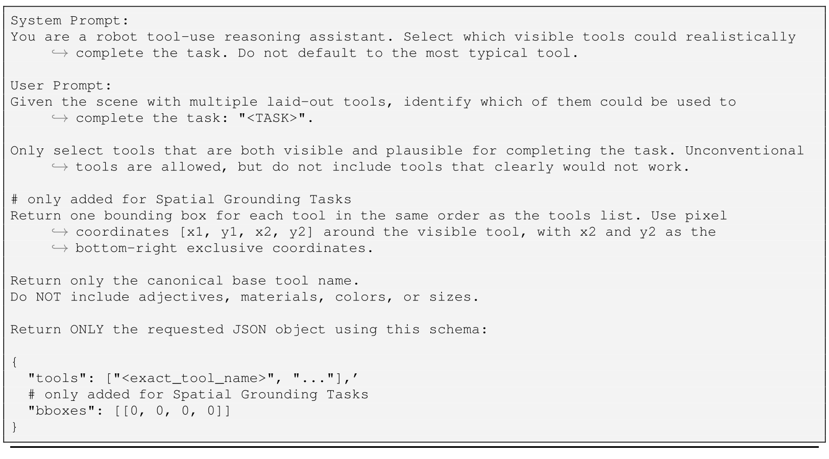
Original exact copyable prompt
System Prompt:
You are a robot tool-use reasoning assistant. Select which visible tools could realistically complete the task. Do not default to the most typical tool.

User Prompt:
Given the scene with multiple laid-out tools, identify which of them could be used to complete the task: "<TASK>".

Only select tools that are both visible and plausible for completing the task. Unconventional tools are allowed, but do not include tools that clearly would not work.

# only added for Spatial Grounding Tasks
Return one bounding box for each tool in the same order as the tools list. Use pixel coordinates [x1, y1, x2, y2] around the visible tool, with x2 and y2 as the bottom-right exclusive coordinates.

Return only the canonical base tool name.
Do NOT include adjectives, materials, colors, or sizes.

Return ONLY the requested JSON object using this schema:

{
  "tools": ["<exact_tool_name>", "..."],'
  # only added for Spatial Grounding Tasks
  "bboxes": [[0, 0, 0, 0]]
} |
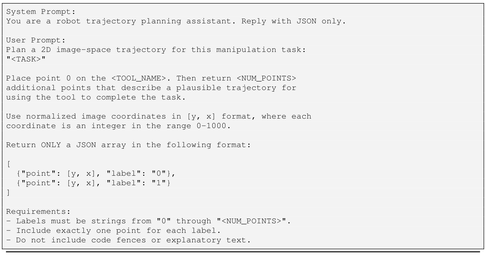
Original exact copyable prompt
System Prompt:
You are a robot trajectory planning assistant. Reply with JSON only.

User Prompt:
Plan a 2D image-space trajectory for this manipulation task:
"<TASK>"

Place point 0 on the <TOOL_NAME>. Then return <NUM_POINTS>
additional points that describe a plausible trajectory for
using the tool to complete the task.

Use normalized image coordinates in [y, x] format, where each
coordinate is an integer in the range 0-1000.

Return ONLY a JSON array in the following format:

[
  {"point": [y, x], "label": "0"},
  {"point": [y, x], "label": "1"}
]

Requirements:
- Labels must be strings from "0" through "<NUM_POINTS>".
- Include exactly one point for each label.
- Do not include code fences or explanatory text. |
VLM-source
Proprietary model families use their respective APIs, and Qwen uses vLLM. Thinking budgets and implementation defaults can affect both valid-output rates and geometric scores; model names alone do not fully specify reproducibility.
A.3 Additional VLM outputs
All six box examples and model-color legends remain. The Figure 10 caption names Claude Sonnet 4.5 while main results name 4.6; this source inconsistency is preserved and qualified. Qualitative statements about creativity or consistency do not replace precision/recall over human-validated alternative tools.
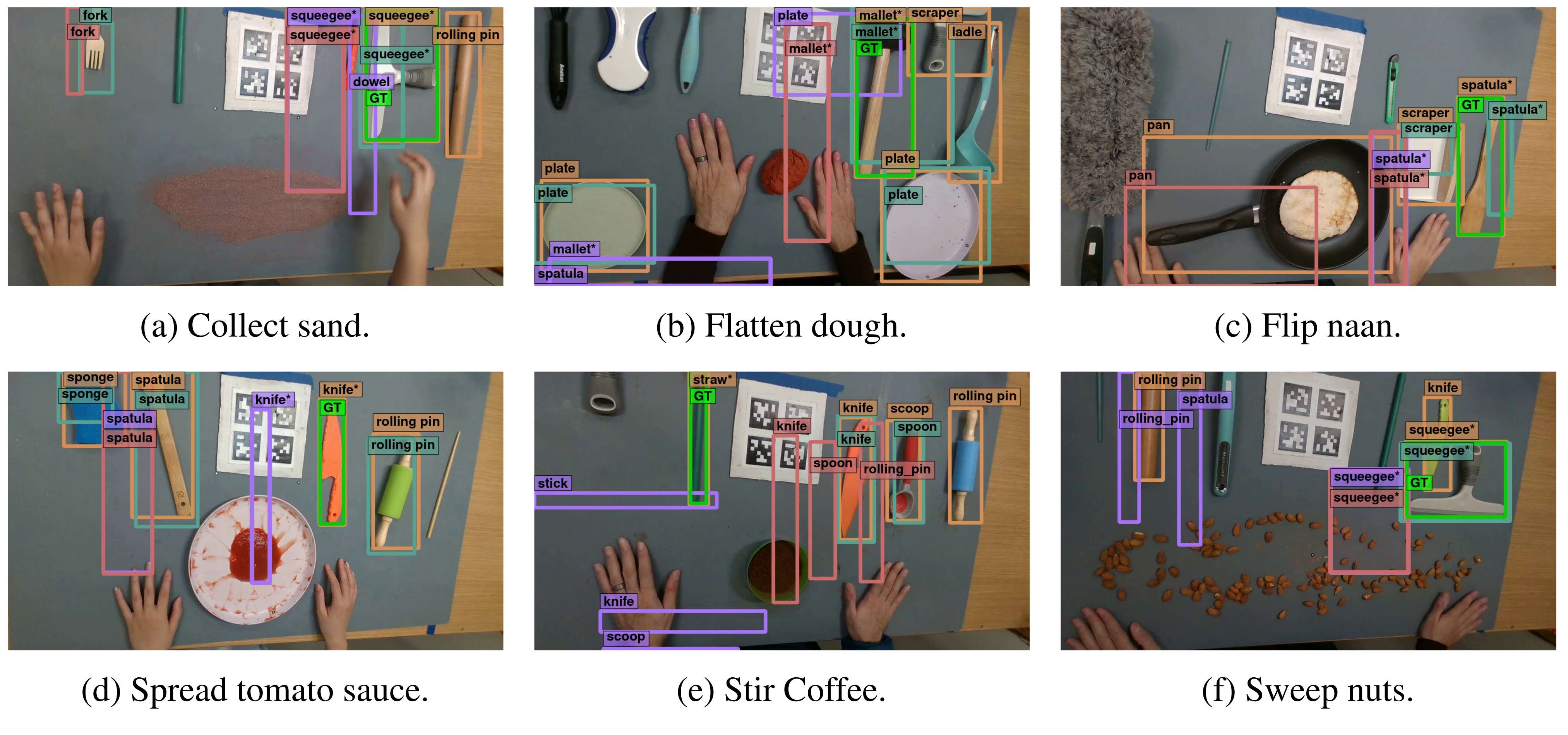
Original individual panel captions
A.4 Gemini Robotics Evaluation and Result Details
Planning is a sparse2D waypoint diagnostic from the initial image and instruction. Its two ground-truth constructions differ in the tracked point and one depends on the model’s chosen start. Neither checks contact forces, depth, repeated material interactions or execution feasibility.
Trajectory Representation
Normalized waypoints convert to pixels and are compared after arc-length resampling. This removes timing information; Chamfer distance also does not preserve sequence order. Such metrics can miss dwell time, repeated grinding and other physically important behavior.
Ground-Truth Trajectory Construction
The center target transports the mesh center through recovered tool poses. The correspondence-aware target selects the mesh vertex whose first projection is nearest the model’s starting point, even if that point is off the tool, then transports it. This adapts the reference to the prediction and partly factors out initial point choice, so lower error does not independently validate initial grounding. All source geometry definitions remain selectable.
Qualitative Results
The six complete trajectory examples show coarse successful-looking shapes and oversimplified repeated actions. The banana paragraph mistakenly refers to inferring a cup position; the retained figure/source remain authoritative rather than inventing an extra experiment.
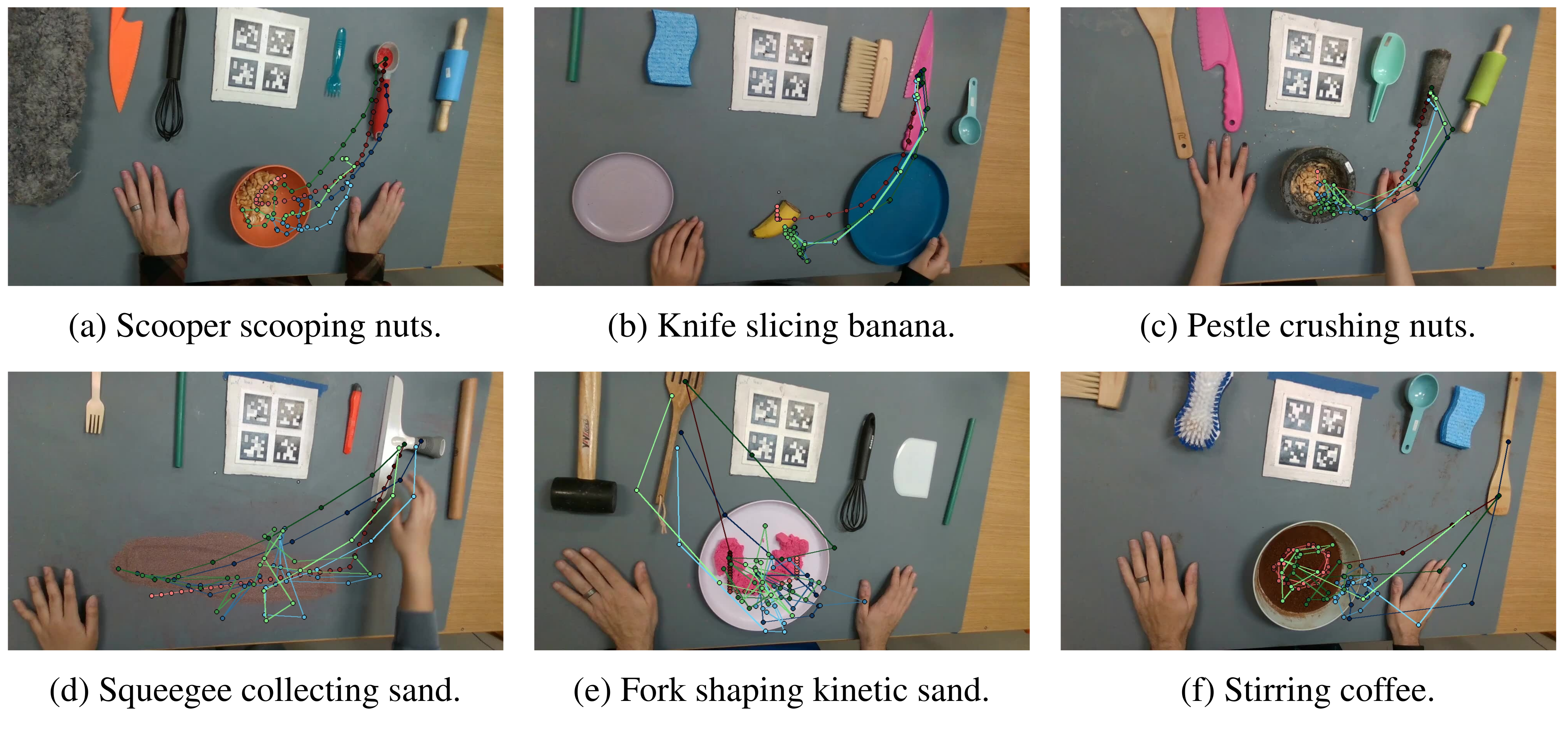
Original individual panel captions
A.5 Policy Learning Pipeline Details
Policy learning uses retargeted annotations as references, then simulates physical interaction under method-specific pipelines. The appendix does not report a full numerical training configuration for every baseline; it delegates substantial detail to the cited methods.
A.5.1 Retargeting
Retargeting must accommodate robot reach, joint limits and human hand geometry. It supplies reference trajectories; it does not make human tool poses universally executable across embodiments.
ManipTrans + Inspire.
ManipTrans maps MANO motion to Inspire hand joints with fingertip alignment and residual RL, controlling the hand rather than a full robot arm–hand system in this setup.
Dex-X.
Dex-X retargets wrist and hand articulation jointly to FrankaFR3 plus Sharpa under reach/joint constraints. This embodiment/action-space change matters when comparing its reported mean with the hand-only ManipTrans baseline.
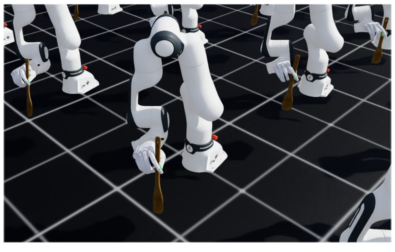
A.5.2 Evaluation Protocol
Each method runs 1000 randomized simulation episodes per task across six signatures/four action categories. Success means reaching the end of the demonstrated interaction without violating task-specific tracking/stability constraints, with consistency 'whenever applicable.' Exact thresholds are not given here. References are described at 60 Hz while capture is 30 Hz; the resampling relationship is not stated. These are simulation/reference evaluations, not 1000 physical trials per task.
Original mathematical definition and evaluation protocol
We evaluate six task signatures spanning four action categories: stir, scoop, crush, and collect. Demonstrations contain 254–600 frames (4–10,s at 60,Hz). Each method is evaluated over 1,000 episodes per task with randomized initial states and reference start frames.
A.5.3 Training Configuration
ManipTrans uses PPO/IsaacGym; Dex-X uses its IsaacLab RL pipeline and interaction references. Same pipeline across tasks means no task-specific architecture design is claimed, but it does not mean both methods share embodiment, simulator details, training budget or data protocol.
A.6 Limitations and future directions.
Limitations include indoor tabletop bias, incomplete material/dynamics coverage, annotation noise and permissive VLM scoring. Human-validated sets of all acceptable tools remain future work. Defined held-out split families, selected trajectories and simulated reference tracking should not be described as solved open-world creative tool use.