At a glance
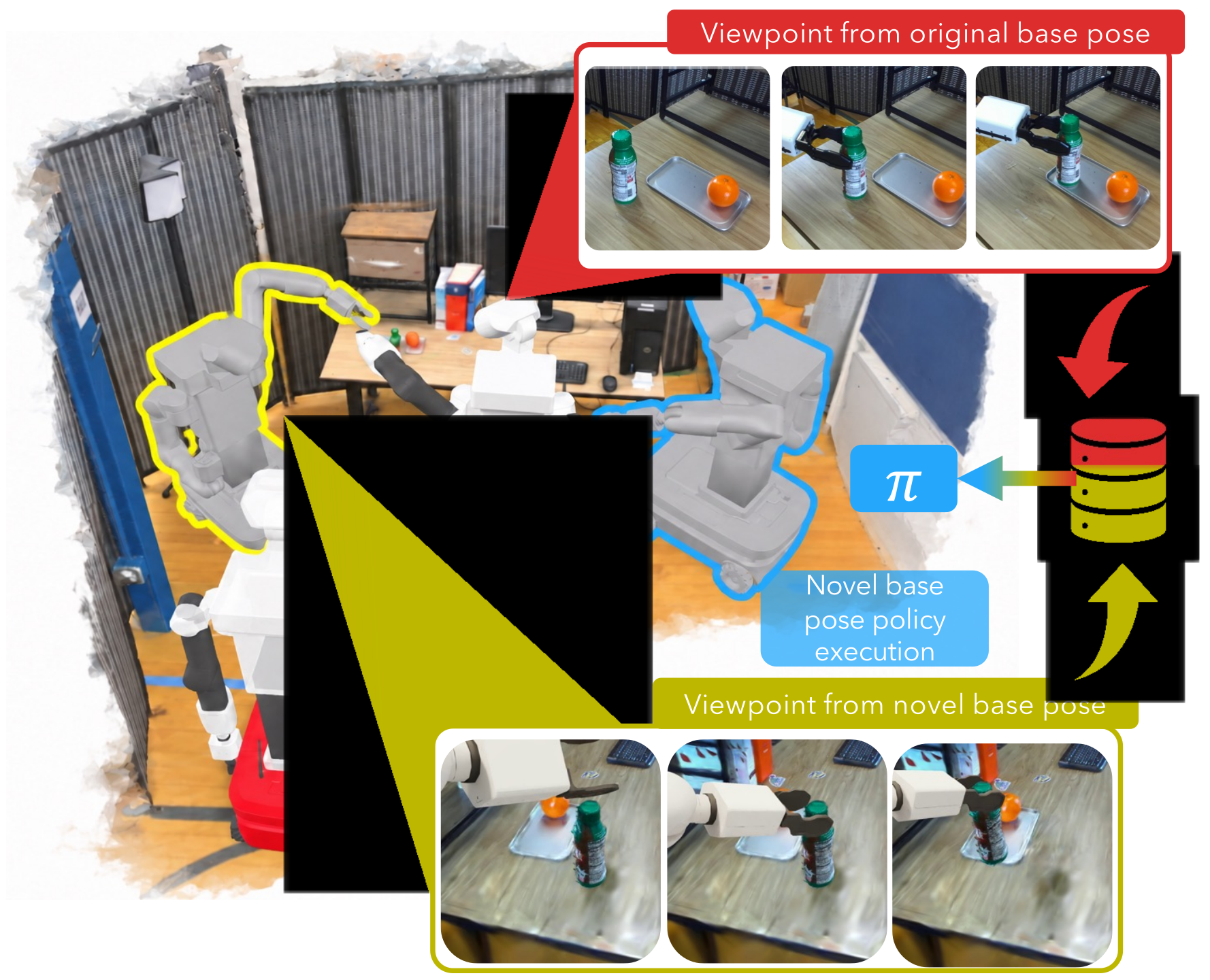
MoMaSplat augments mobile-manipulation demonstrations by reconstructing the stationary scene and moving object separately, then rendering both together with a retargeted robot at new base poses. Navigation supplies scene views and a common alignment reference; manipulation supplies object motion. Across five physical tasks, mean success at unseen base poses rises to 37%, compared with 17% for the strongest tested baseline. This is a substantial improvement from a low baseline, not reliable general-purpose mobile manipulation. The edition preserves all five numbered figures, both tables, the original displayed formulas and the full implementation appendix.
I INTRODUCTION
A mobile robot rarely stops at exactly its demonstration location. Even a modest displacement changes both camera appearance and the base-relative action frame, so fixed-view imitation can fail despite arm reachability. Existing novel-view augmentation often treats the manipulated object as static, leaving post-contact motion inconsistent. MoMaSplat uses ordinary navigation and manipulation recordings to reconstruct that motion, synthesize full visual trajectories and transform action/proprioception labels together. It broadens the training distribution around demonstrated poses rather than selecting a perfect deployment pose or collecting real demonstrations everywhere.
II Related Work
Simulation-based demonstration synthesis needs modeled environments/dynamics or verification rollouts; generative video augmentation can introduce geometry errors. Static novel-view methods cannot independently move the object after contact. The proposed contribution combines real-scene/object reconstruction with simulation only for the known robot appearance. Unlike Mobi-π, which seeks base poses compatible with a policy’s existing distribution, it trains a policy over a wider pose distribution. This comparison concerns the evaluated implementations: the One-Thousand Trajectories baseline omits that method’s additional trajectory augmentation, as detailed in Appendix A.
III MoMaSplat
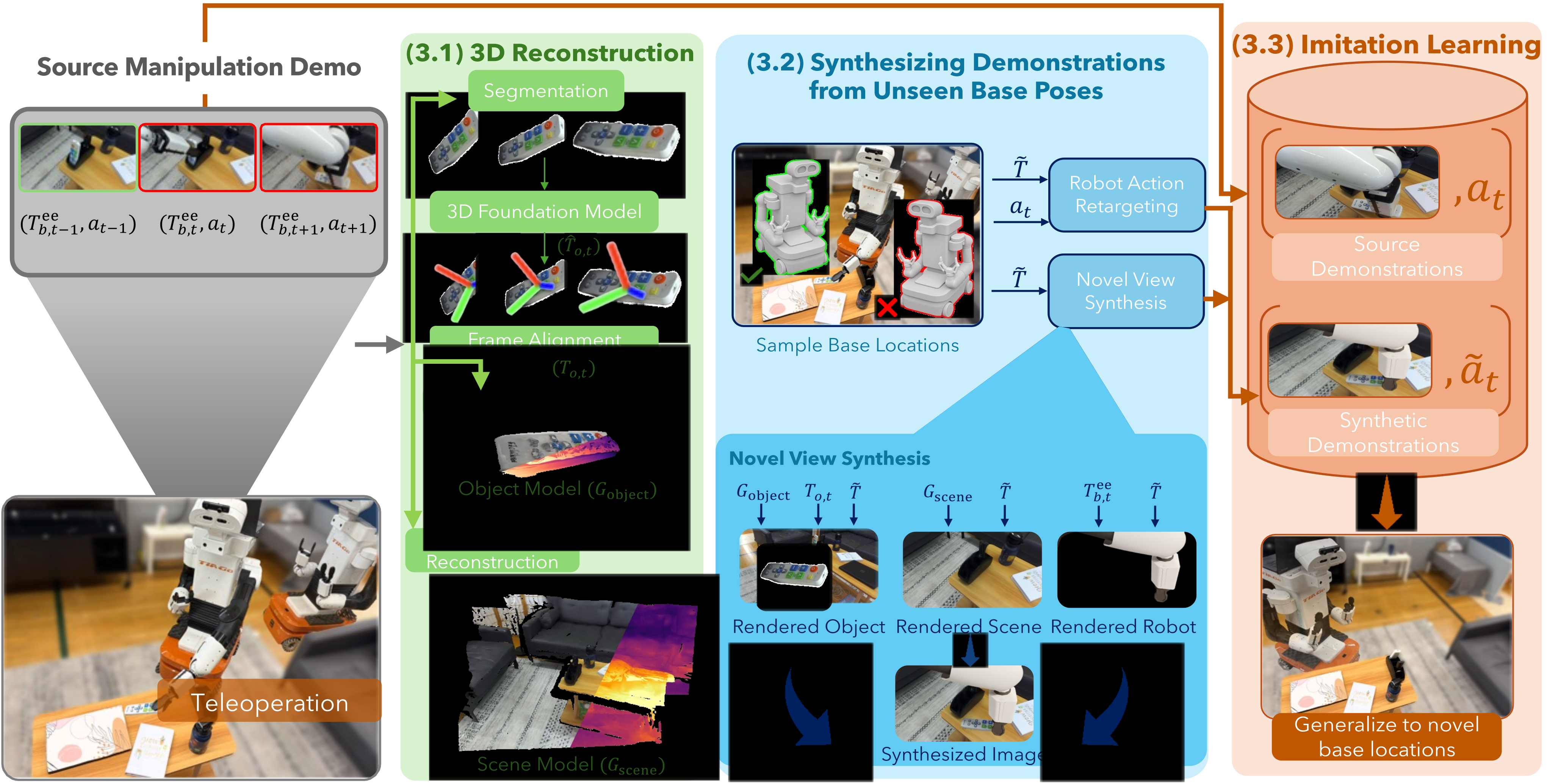
The robot navigates between planar base poses, then manipulates with its base fixed. Navigation RGB/state sequences observe an unmoving object; manipulation demonstrations contain RGB, robot state and seven-dimensional end-effector translation/rotation deltas plus a gripper command, expressed in the base frame. Three separately rendered components—scene, object and robot—share metric coordinates. A source demonstration is replayed from each feasible sampled base pose, preserving the demonstrated world-relative end-effector/object motion. The generated observations and transformed labels are added to the real data. The approach augments where execution begins, not the physical interaction strategy itself.
Equation
III-A 3D Reconstruction
COLMAP estimates navigation-camera poses and a sparse scene cloud, followed by uncertainty-aware WildGaussians reconstruction. Object and rendered-robot masks prevent those components from being baked into the stationary scene. Depth measurements recover metric scale through robust measured/rendered depth ratios. For the moving object, segmented RGB views feed FastVGGT, producing camera poses relative to the object without a pre-existing object model. Navigation frames provide the bridge: because the object is then stationary, their object-relative and scene-relative camera trajectories differ only by a similarity transform. Umeyama alignment maps the object reconstruction into the metric scene frame; Gaussian appearance and poses are then jointly refined. An articulated object is represented by its moving rigid link, while the stationary remainder belongs to the scene. The method does not estimate joint parameters or extrapolate articulation beyond the demonstrated motion.
III-B Synthesizing Demonstrations from Unseen Base Poses
Sample planar offsets around the original base, aim toward the object and add heading noise; reject poses failing visibility or inverse-kinematics checks at selected trajectory times. Transform end-effector poses by the original-to-sampled base transform to preserve their world pose. Render the scene splat, moving object splat and inverse-kinematically retargeted simulated robot separately, then composite their RGB/depth/opacity layers front-to-back per pixel. Both labels and proprioception must follow the new frame: translation deltas rotate by the base-frame rotation; rotation deltas are conjugated, equivalently rotating the axis while keeping the axis-angle magnitude. Absolute end-effector pose receives the full rigid transform; gripper state/command stay unchanged. Generate K variants per source trajectory. Probe-time IK establishes sampled reachability, not complete contact-dynamics or collision feasibility, and the object still follows its recorded trajectory.
III-C Imitation Learning
The same Diffusion Policy architecture is trained on real and generated demonstrations using the original noise-prediction objective. It conditions on egocentric RGB and end-effector proprioception and predicts a sequence of pose-delta actions. A weighted sampler selects real sequences with probability 0.25 and synthetic sequences with probability 0.75; this deliberate sampling balance differs from the raw one-to-ten dataset-size ratio.
Equation 1
| (1) |
IV Experimental Evaluation
Evaluation separates downstream policy robustness from image-generation fidelity. Real-robot tests measure success after unseen base placement, with additional source-data ablations. Simulation provides exactly corresponding trajectories, camera poses and object motion for assessing synthesized observations; a newly teleoperated real trajectory would not be identical ground truth. Image quality and task success therefore answer different questions.
IV-A Experimental Setup
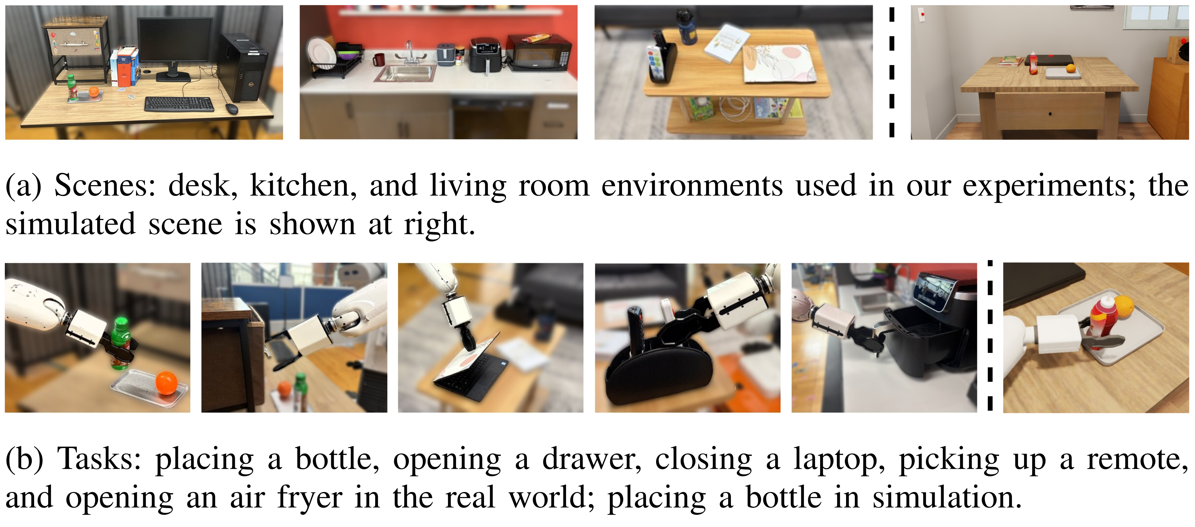
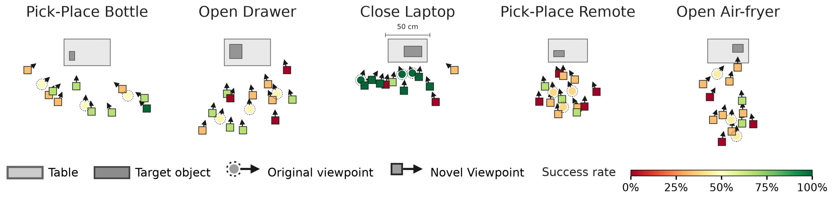
Five TIAGo tasks span three scenes: bottle placement and drawer opening at a desk, remote placement and laptop closing in a living room, and air-fryer opening in a kitchen. Collect 75 laptop demonstrations and 90 for each other task across three base poses, plus nine navigation trajectories. Each method receives the same real demonstrations; each task is evaluated at 12 unseen base poses with three trials per pose. MoMaSplat samples a 1.2 m square around each source pose and generates ten synthetic demonstrations per original. One-Thousand Trajectories receives the same action retargeting but only 400 synthetic bottle demonstrations because its static object reconstruction matches only 40 of the 90 originals; all 90 real demonstrations remain available. Other augmented datasets contain 750–900 sequences. A separate simulated bottle task follows the real task structure without matching its exact geometry.
IV-B Results
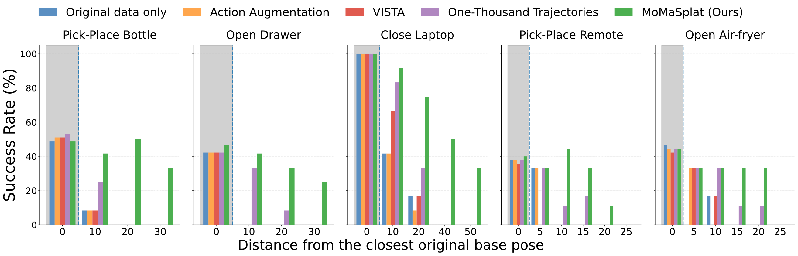
Across the five tasks, unseen-pose success is 37% for MoMaSplat, 17% for One-Thousand Trajectories, 8% for VISTA and 6% each for real-only training and action-noise augmentation. Original poses receive 15 trials each and are comparable across methods. At larger offsets, reported examples include 33% bottle success at 30 cm and 50% laptop success at 40 cm, where tested baselines reach zero. With 10, 50 and 90 source bottle demonstrations, success at four 10–20 cm test locations is 33%, 42% and 50%; 90 real-only demonstrations yield 8%. These are limited task/pose trial counts, not uncertainty-qualified evidence of deployment reliability.
Generation fidelity uses 75 simulated trajectories, sampling every tenth frame for 2,486 image comparisons; static-scene evaluation uses only one view per trajectory. Table I preserves PSNR, SSIM and LPIPS for the full image and segmented scene/object/robot. Mean PSNR is 21.27 dB overall, 26.40 for scene, 18.18 for object and 17.43 for robot. The evaluated view displacement is 0.4–27.3 cm from reconstruction views, a different distance definition from base-pose policy evaluation. Across 30 source trajectories, estimated object poses have 1.46 ± 0.71 cm translation and 4.01 ± 4.66° rotation error. Real held-out scene PSNR is 24.00 dB over 110 frames; object crops score 23.63 dB at registered poses and 22.59 at interpolated poses. Real full-image scores are omitted because simulated/real robot appearance differs. The paper’s comparison with another dataset’s 3DGS PSNR is contextual, not a controlled benchmark.
| Region | PSNR (dB) | SSIM | LPIPS |
|---|---|---|---|
| Full image | |||
| Scene | |||
| Object | |||
| Robot |
V Conclusion and Limitations
Separating stationary scene, moving rigid object and robot permits coherent post-contact viewpoint augmentation and improves the tested policies. Important gaps remain: predominantly static surroundings, reliable masks, adequate navigation coverage and visible rigid surfaces are required. Texture-poor, occluded or deformable objects are challenging. Surfaces hidden behind the initial object—such as a bottle’s support surface or an opened container’s interior—were never observed in masked scene reconstruction and remain unmodeled when revealed. Replaying object motion does not simulate contact forces or dynamics. Dynamic backgrounds, clutter, deformability and physical interaction remain future work; the source promises code release without making it part of this review.
Acknowledgment
The work was conducted in UT Austin’s RobIn Lab, with support acknowledged from NSF, NVIDIA, Amazon and DARPA TIAMAT. Additional author support includes NSF/NVIDIA grants and an Amazon AI PhD fellowship; the stated findings are the authors’ rather than the sponsors’ views.
-A Baseline Details
Real-only and action-noise baselines use the same policy and training schedule. Action augmentation changes proprioception/labels but leaves images unchanged. VISTA uses released ZeroNVS independently per frame at 256² resolution: planar offsets within ±10 cm, object-directed yaw clipped to ±0.5 rad, 50 DDIM steps with η=0, guidance 7.5 and 70° field of view. Larger perturbations produced artifacts; original actions remain unchanged, and independent synthesis is temporally inconsistent. One-Thousand Trajectories uses the same navigation-based static reconstruction pipeline without masking out the object, plus MoMaSplat’s action retargeting. Its separate trajectory-augmentation component is not used. For bottle manipulation, only the 40 originals matching its reconstructed initial object pose produce 400 synthetic sequences, while all 90 originals train the policy.
-B Method Details
Implementation details clarify how reconstruction achieves metric consistency despite sparse object keyframes, imperfect segmentation and pose-estimation noise. Both reconstruction streams require additional geometric refinement; the feed-forward object model alone is not the final trajectory estimator.
-B -1 3D Scene Model Reconstruction
Sequential COLMAP matching uses navigation images plus a few pre-manipulation context frames. WildGaussians trains for 30,000 iterations with appearance/exposure embeddings, DINOv2-based uncertainty and DSSIM weight 0.2; every eighth frame is held out. Metric scaling takes the median valid measured/rendered depth ratio per frame and then the median across frames, using measured depths in (0,9] m and at least 1,000 valid pixels per frame. Unregistered navigation poses use the object pipeline’s interpolation and outlier filtering. These details explain the depth-sensor requirement even though policy inputs are RGB and proprioception.
-B -2 3D Object Model Reconstruction
GroundingDINO localizes text-named objects; SAM2 propagates masks forward and backward from a seed frame. Overlapping object masks lose contested pixels, and scene training excludes both object and simulated-robot masks. Roughly 10–20 motion-diverse frames per demonstration survive small-mask filtering and a bounding-box IoU<0.8 or >20-frame-gap rule; endpoints remain. Add 50 navigation frames and cap the feed-forward input at 400 frames per object. FastVGGT supplies poses, intrinsics and depth; dense tracks and bundle adjustment enforce multiview consistency, requiring points in at least two views and adaptive reprojection filtering.
Camera-center alignment uses Umeyama within RANSAC: five-camera subsets, plausible-scale rejection, 0.2 m inlier tolerance, highest-consensus refitting and Huber refinement; Table II specifies 8,000 trials. gsplat then optimizes object appearance for 60,000 steps using masked RGB/opacity supervision, L1 plus SSIM weight 0.2 and pose learning rate 10⁻⁵. To recover every demonstration timestep, interpolate rotations with SLERP and translations linearly after suppressing small jitter and spurious A→B→A excursions. An ease-in timing map concentrates motion toward interval ends. These heuristics can shape reconstructed motion and are not a learned dynamics model.
-C Base Pose Sampling Strategy
Sample around each source demonstration’s reconstructed world-frame base pose, normally uniformly over a square; an annular bounded-Gaussian option is also described. Aim the fixed head camera toward the object centroid while accounting for the camera/base offset, then add up to ±20° heading noise. Reject near-edge or invisible objects before the costlier IK test. cuRobo checks multiple demonstration timesteps inside OmniGibson; every probe must be reachable, with rejected poses resampled up to a fixed draw budget until K accepted poses are collected. No continuous-trajectory contact or dynamics validation is claimed.
| Stage | Parameter | Value |
|---|---|---|
| Scene SfM | matcher | sequential (COLMAP) |
| Scene 3DGS | method / iterations | WildGaussians / |
| Scene 3DGS | DSSIM weight | |
| Metric scale | valid-depth range | m, px/frame |
| Segmentation | detector / tracker | GroundingDINO / SAM2 |
| Frame selection | IoU thresh. / max gap | / frames |
| Frame selection | VGGT input budget | frames per object |
| Object BA | visibility per 3D point | views |
| RANSAC | subset / trials / inlier | / / m |
| Object 3DGS | steps / SSIM weight | / |
| Object 3DGS | pose-opt learning rate | |
| Base sampling | region / yaw noise | cm / |
| Generation | synthetic per source demonstration | |
| Policy | obs / action horizon | / |
| Policy | DDIM train timesteps | |
| Policy | optimizer / learning rate | AdamW / |
| Policy | batch size / training steps | / |
| Policy | source : generated ratio |
-D Imitation Learning
A conditional one-dimensional U-Net uses a from-scratch ResNet-18 image encoder and spatial softmax with 32 keypoints, concatenated with end-effector state. It stacks two observations at 224² pixels and predicts eight normalized seven-dimensional actions. Training applies crop, translation and color jitter. DDIM uses 50 training and inference denoising steps, a cosine noise schedule and noise-prediction loss. AdamW trains for 100,000 steps, batch 32, learning rate 3×10⁻⁴, weight decay 10⁻⁴, cosine decay and 1,000 warmup steps. Real/synthetic sampling is 0.25/0.75. The TIAGo’s head RGB-D camera has 70° field of view; the policy uses RGB, while depth calibrates reconstruction scale. Table II retains the full pipeline settings.