Overview
This edition covers all 22 pages, including Appendices A–J, the complete notation table, five figures, nine numbered tables and original project clips. The method communicates environmental preferences for two sequential robots with separate policies/tasks; the shared state representation, follower initial state and model access are substantive assumptions.
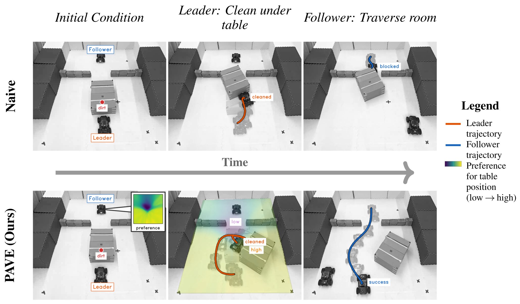
At a glance
Policy Adaptation via Value Exchange lets a leader use a fixed follower’s learned value function to plan a better workspace handoff. A nearest-neighbor support filter reduces reliance on unfamiliar states, and CEM adapts the leader online from its own policy prior. Follower gains average 27.9 percentage points over five simulation scenarios, reaching 48.5 points; separate hardware gains are 40 points over twenty matched configurations per method. These results support useful ad hoc coordination, without a formal guarantee of preserved individual success or calibrated value uncertainty.
Original mathematical definition and qualification
We consider the problem of sequential task continuation, where one robot acts in a workspace that has been affected by a previous robot.
Current approaches in multi-robot cooperation rely heavily on co-training or co-optimization, assuming that the robots have access to collective interaction data during the policy training or planning process. However, as increasingly varied robotic embodiments and policies are deployed and operate in the same real-world environment, learning policies for cooperation becomes infeasible due to the combinatorial explosion of possible robot combinations that need to be accounted for. To address this challenge, this paper considers the problem of ad hoc sequential cooperation between robots that have never before operated together in a shared environment. We demonstrate that robots can explicitly communicate their environmental preferences through sharing their value functions, enabling coordination without the need for prior joint training. To ground this exchange and prevent overconfidence in out-of-distribution states, we further introduce a -nearest neighbors (KNN)-based uncertainty filter. Our method yields an increase of up to 48.5 pp compared with naive or even selfish agents, in task success rates across simulated and real-world experiments, demonstrating that value function transmission between agents is useful not merely as an internal learning tool, but as an effective basis for ad hoc coordination.
Website: https://proroklab.github.io/PAVE/
1 Introduction
Independently trained robots can interfere by rearranging a workspace before another robot arrives. Sharing a follower’s environmental value gives the leader an explicit handoff preference without co-training every pairing. The setting concerns distinct tasks in a known sequential order, with direct communication and a common world representation. Avoiding pair-specific training still requires independently capable policies, critics, normalization data and follower-distribution support information.
Original mathematical definition and qualification
An uncertainty-based grounding using a -nearest-neighbors distribution filter to prevent the receiving agent from acting on unreliable value estimates.
Related Work
Ad hoc/zero-shot teams, consecutive-policy training and environment co-design provide related coordination mechanisms. PAVE adapts online through a learned value interface and physical environmental changes, with a fixed follower and separate embodiments/action spaces. Finetuning is inspired by prior consecutive-policy work rather than being its exact reproduction.
2 Problem Statement
The leader controls the distribution of terminal shared states handed to a fixed follower. The objective sums leader return and alpha-weighted follower return under that handoff distribution. Private states, rewards and policies remain agent-specific, while both robots share w. This weighted objective permits tradeoffs; it contains no explicit constraint that either agent must retain its baseline success. Formal expected-return definitions and all initial distributions remain selectable.
Original mathematical definition and qualification
Setting. More generally, we consider cooperation problems in which agents act sequentially in the same environment. We call the first agent the leader and the second agent the follower . Both share a common representation of their environment as well as individual private states and . They act according to policies and with reward functions . Their expected returns are , where and are the initial distributions of the leader’s and follower’s private states, respectively, is the initial distribution of the environment state, and is the discount factor. The follower’s expectation conditions on , i.e. the handoff state passed in from the leader.
Original mathematical definition and qualification
Sequential Subtask Execution. The leader acts in the environment for steps leaving behind a terminal environment state distributed according to the handoff distribution , which depends only on the leader policy and world dynamics.
Original mathematical definition and qualification
Cooperative Leader. To achieve meaningful cooperation, the leader cannot strictly maximize its own return, . It must concurrently optimize for the follower’s expected return given the inherited environment state. Because the leader’s influence on the follower is solely dictated by the handoff distribution, , the joint cooperative objective becomes
Equation 1
| (1) |
Original mathematical definition and qualification
with weight . The follower policy is assumed to be fixed, reacting only to the handoff state that the leader leaves behind.
Original mathematical definition and qualification
Modular Composition As this work focuses on ad hoc coordination, we assume that collective interaction data is not accessible prior to deployment. This requires the leader to solve (1) online during deployment. Further, the leader needs to evaluate the follower’s performance under arbitrary environment states , requiring detailed knowledge about the follower’s behavior, its interaction dynamics with the environment, and its reward function to simulate its response to the leader’s behavior when planning. We address this problem in the following section by introducing a simplified preference interface that abstracts this complexity and is easy to obtain.
3 Method
An exact environmental value equals the fixed follower’s expected return from a handoff state. In practice the paper uses a PPO critic at a known follower initial private state; marginalizing a distribution is described but not evaluated. A learned critic approximates that equality. Sharing it avoids explicitly simulating the follower’s policy, but does not itself prove privacy or prevent information leakage through value queries.
Original mathematical definition and qualification
Modularity stems from abstraction through common interfaces. We propose using the value function as an abstraction for coordination. The value function of a policy maps states to expected returns under that policy. Because agents in a shared environment operate on a common environment state , the environmental value function naturally serves as a preference function, communicating how desirable a given environment state is to the follower. By construction, , meaning it equals the follower’s expected return from the handoff state . Substituting into (1), the cooperative objective becomes
Equation 2
| (2) |
Original mathematical definition and qualification
By revealing its value function, the follower enables the leader to optimize (2) on its behalf without requiring any further input. In practice, we obtain the environmental value function by aggregating the critic of an agent trained with PPO [28]. The critic depends on the full follower state , comprising the follower’s private state and the environmental state . Since the leader optimizes only over , we aggregate the critic to produce the environmental value function — either by fixing the initial private state to a known value (), or by taking the expectation over the follower’s initial private state distribution . In this work, we only consider the case of a known initial state for the follower. Because PAVE shares only , the leader cannot recover without an additional model of the follower’s private state and dynamics. Specifically, does not expose the follower’s individual state or action distribution.
Cooperative Objective
Prior-policy rollout ranges normalize the two returns before a weighted sum; deployment uses alpha four. This establishes a domain-specific tradeoff rather than a universal preference scale. The reported normalization maps prior observations to a reference range; novel critic predictions need not remain bounded within it. Constants and all original formulas are retained.
Original mathematical definition and qualification
Combining two qualitatively different objectives is nontrivial and domain-dependent. The proposed approach allows for the selection of arbitrary aggregation functions. In this work, we combine the two objectives by first normalizing them and then summing them using a weighting factor, .
Equation 3
| (3) |
Original mathematical definition and qualification
where are determined from rollouts of the leaders’ and followers’ prior policies.
Uncertainty-Aware Value Interface
The OOD score clips normalized mean distance to five neighboring follower-training states. Thresholds use the 95th and 99.9th percentiles over a thousand sampled training-distribution states. It measures representation density, not a calibrated probability of value error or a safety certificate. Deployment needs a shareable support/uncertainty computation in addition to the value interface. State scaling, neighbor self-exclusion and a degenerate equal-percentile fallback are not fully specified in the manuscript.
Equation 4
| (4) |
Original mathematical definition and qualification
is close to zero when environment states are near the training samples on which the follower was trained, and becomes large when they are far away. This can be leveraged to adjust the value function in regions of the state space where the agent, and therefore its value function, has not been trained. We choose . The parameters and are chosen to be, respectively, the 95th and 99.9th percentiles of the empirical distribution of the mean distance to the nearest neighbors of each state, computed over a sample of 1000 states drawn from the environmental state distribution on which the follower was trained.
Cooperative Online Planning
CEM samples leader action sequences, warm-started by its own frozen policy, and replans over a finite horizon. Follower value and support are evaluated at the horizon endpoint, a proxy for the eventual handoff. Leader rewards bootstrap from its own critic, whose selfish-prior continuation can differ from the adapted continuation. The sign of this learned-tail error is not guaranteed without an optimal/exact selfish value. Equation 6’s reward indexing and boundary bootstrap need a consistent implementation convention; the exact published expression remains intact. The multi-agent-chain remark is conditional on baseline-preservation guarantees that this weighted approximate planner does not establish or test.
Original mathematical definition and qualification
To enable ad hoc cooperation, the planning procedure must be computationally feasible online. Because trajectory optimization benefits significantly from a strong prior, we use the leader’s independently trained policy to warm start the search. At each step, the planner seeks to maximize the normalized, uncertainty-aware cooperative objective:
Equation 5
| (5) |
Original mathematical definition and qualification
We execute the planner in a receding-horizon fashion at a given time , planning over a horizon of time steps and predicting future states and rewards using a zero-order model of the system dynamics and reward, as our method does not rely on gradient-based optimization. Because the time horizon is limited, we must estimate the leader’s full return, , by approximating the tail rewards.
Equation 6
| (6) |
Original mathematical definition and qualification
This limited horizon requires two practical approximations. First, because the true terminal handoff state is unavailable at time , we use the environment state at the end of the horizon, , as a proxy to evaluate both the follower’s value function and the uncertainty penalty . Second, using as an infinite-horizon value approximation introduces a non-cooperative baseline bias: assumes the leader will act purely selfishly beyond the horizon, yielding an overestimate of the true return, since the online policy may actually continue sacrificing some reward to aid the follower. Empirically, however, neither the state proxy nor the terminal value approximation adversely impacts the performance of either agent. To solve the optimization problem (5) online, PAVE employs the Cross Entropy Method (CEM) [27] over the receding horizon. A detailed listing of parameter values is provided in Appendix F.
Original mathematical definition and qualification
Remark: This methodology extends to arbitrary sequences of agents through recursive pairwise application. For an ordered sequence of agents , each agent treats agent as its immediate follower, adapting its policy to the successor’s value function . Provided that the two-agent formulation guarantees the leader preserves the follower’s baseline performance, this framework can be applied transitively to guarantee cooperative behavior across the entire -agent chain.
4 Experimental Analysis and Real-world Deployment
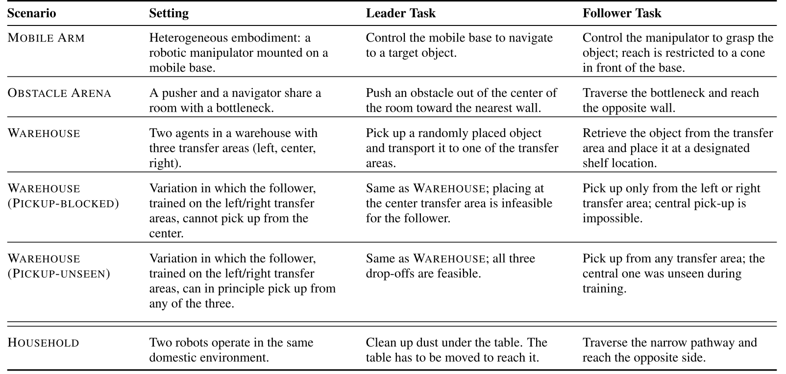
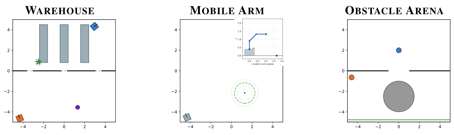
Five custom simulation variants arise from three underlying layouts; Household is hardware-only. Leader-only planning, removal of the OOD filter or prior, and a privileged finetuning comparison isolate selected components. Naive is a reference policy, not a mathematical lower bound for every approximate planner. Finetuning uses extra joint rollout data and 1.5M updates, with its separately selected alpha one rather than PAVE’s four.
Accessible table, original values and mathematical notation
| Scenario | Setting | Leader Task | Follower Task |
| Mobile Arm | Heterogeneous embodiment: a robotic manipulator mounted on a mobile base. | Control the mobile base to navigate to a target object. | Control the manipulator to grasp the object; reach is restricted to a cone in front of the base. |
| Obstacle Arena | A pusher and a navigator share a room with a bottleneck. | Push an obstacle out of the center of the room toward the nearest wall. | Traverse the bottleneck and reach the opposite wall. |
| Warehouse | Two agents in a warehouse with three transfer areas (left, center, right). | Pick up a randomly placed object and transport it to one of the transfer areas. | Retrieve the object from the transfer area and place it at a designated shelf location. |
| Warehouse (Pickup-blocked) | Variation in which the follower, trained on the left/right transfer areas, cannot pick up from the center. | Same as Warehouse; placing at the center transfer area is infeasible for the follower. | Pick up only from the left or right transfer area; central pick-up is impossible. |
| Warehouse (Pickup-unseen) | Variation in which the follower, trained on the left/right transfer areas, can in principle pick up from any of the three. | Same as Warehouse; all three drop-offs are feasible. | Pick up from any transfer area; the central one was unseen during training. |
| Household | Two robots operate in the same domestic environment. | Clean up dust under the table. The table has to be moved to reach it. | Traverse the narrow pathway and reach the opposite side. |
Original mathematical definition and qualification
PAVE (w/o ). The proposed planner with an uninformed prior policy. This serves as an ablation to assess the effectiveness of using the leader’s prior policy to guide the planning process.
5 Results
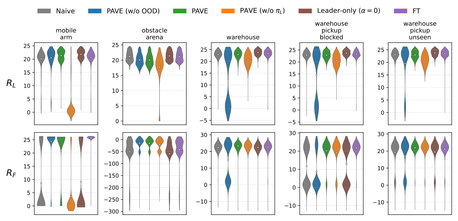
Across five simulation settings, follower gains over Naive are 48.50, 37.83, .45, 40.16 and 12.78 points, averaging 27.94. The 27.9-point headline therefore matches simulation only; including hardware’s separate 40-point gain would give a different mean. Leader success is preserved or improved over Naive in these reported means, while leader-only planning can be slightly higher. Removing OOD badly harms the warehouse family, but improves Mobile Arm (93.83 versus 81.17%) and slightly Obstacle Arena, showing conservatism can discard useful extrapolation. PAVE trails privileged finetuning in two scenarios. Six-seed standard deviations describe retained competent training/evaluation runs, not an unconditional guarantee. Hardware raises follower/joint success from 6/20 to 14/20 on matched starts, with leader 20/20 for both; paired outcome counts are not reported, so no paired significance claim is added.
Original mathematical definition and qualification
Using the leader’s prior as a planning initialization never hurts and helps substantially on constrained tasks. PAVE generally outperforms PAVE (w/o ). Mobile Arm and Obstacle Arena benefit the most from the initial guess. Empirically, we conclude that using the leader’s prior policy as an initial guess for the optimization often improves overall performance and never impairs it.
Original mathematical definition and qualification
Follower gains stem from value exchange and not from online planning alone. Leader-only improves leader success by up to pp but yields no consistent follower gain, recovering at most of PAVE’s follower improvements on the four scenarios where PAVE has headroom. Therefore, PAVE’s follower gains stem primarily from value exchange, not online planning.
Original mathematical definition and qualification
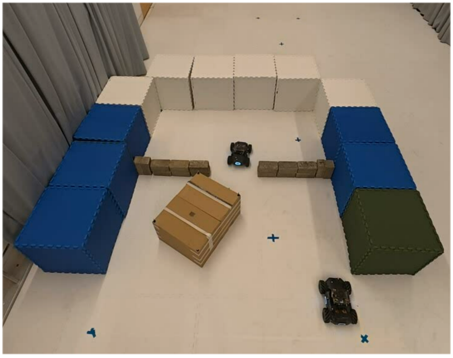
PAVE transfers from simulation to a physical household setup. In deployments with randomized initial conditions, we compare the performance of the NAIVE baseline with our PAVE method, running online in the Household scenario (Figure 1). With both NAIVE and PAVE, the leader succeeds in every instance; however, PAVE increases the follower’s success rate by pp. The real collision dynamics differ substantially from those in simulation (which assume no friction and simple velocity matching), highlighting the strength of online replanning in compensating for prediction error.
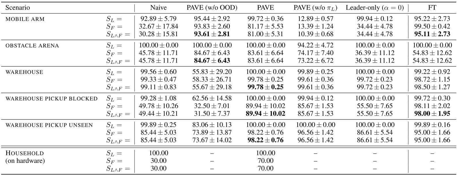
Accessible table, original values and mathematical notation
| Scenario | Naive | PAVE (w/o OOD) | PAVE | PAVE (w/o ) | Leader-only () | FT | |
| mobile arm | 92.89 5.79 | 95.44 2.92 | 99.72 0.36 | 12.89 0.57 | 99.94 0.12 | 95.22 2.73 | |
| 32.67 17.84 | 93.83 2.60 | 81.17 5.53 | 13.39 1.24 | 34.44 4.78 | 99.50 0.42 | ||
| 30.28 15.81 | 93.61 2.81 | 81.00 5.31 | 10.39 0.68 | 34.44 4.78 | 95.11 2.73 | ||
| obstacle arena | 100.00 0.00 | 100.00 0.00 | 100.00 0.00 | 94.22 4.72 | 100.00 0.00 | 100.00 0.00 | |
| 45.78 11.71 | 84.67 6.43 | 83.61 6.64 | 74.17 7.40 | 36.39 11.12 | 54.83 12.62 | ||
| 45.78 11.71 | 84.67 6.43 | 83.61 6.64 | 73.22 6.72 | 36.39 11.12 | 54.83 12.62 | ||
| warehouse | 99.56 0.60 | 55.83 29.20 | 100.00 0.00 | 99.89 0.25 | 100.00 0.00 | 99.22 0.92 | |
| 99.33 0.47 | 58.33 26.71 | 99.78 0.25 | 99.61 0.36 | 99.72 0.23 | 98.72 1.15 | ||
| 99.11 0.83 | 55.67 29.18 | 99.78 0.25 | 99.61 0.36 | 99.72 0.23 | 98.50 1.27 | ||
| warehouse pickup blocked | 99.28 1.08 | 62.56 14.58 | 100.00 0.00 | 99.94 0.12 | 100.00 0.00 | 99.72 0.30 | |
| 49.78 10.26 | 32.50 7.01 | 89.94 10.02 | 85.67 1.53 | 55.50 7.65 | 98.11 2.02 | ||
| 49.44 10.21 | 31.50 7.37 | 89.94 10.02 | 85.67 1.53 | 55.50 7.65 | 98.00 1.95 | ||
| warehouse pickup unseen | 99.89 0.25 | 83.06 10.13 | 100.00 0.00 | 100.00 0.00 | 100.00 0.00 | 99.89 0.16 | |
| 85.44 5.03 | 73.89 13.87 | 98.22 0.76 | 96.56 1.42 | 86.61 5.54 | 95.00 1.66 | ||
| 85.44 5.03 | 73.67 14.02 | 98.22 0.76 | 96.56 1.42 | 86.61 5.54 | 95.00 1.66 | ||
| Household | 100.00 | – | 100.00 | – | – | – | |
| (on hardware) | 30.00 | – | 70.00 | – | – | – | |
| 30.00 | – | 70.00 | – | – | – |
6 Conclusion
Value exchange can guide a leader toward useful handoffs without pairwise joint training, but the tested setting is two robots in predetermined order. Shared world coordinates, truthful messages, a capable follower/critic and a useful short-horizon model are prerequisites. No policy-invariance, hard safety or arbitrary-chain guarantee follows from the empirical results. Longer horizons, unknown followers and incompatible representations remain open.
Original mathematical definition and qualification
Limitations and Future Work This work focuses on two agents acting sequentially in a pre-defined order. One axis of future research lies in the number of possible followers. If the sequence of agents acting in the environment is either unknown or not predetermined, one leader could adapt to the needs of multiple followers; a possible solution is optimizing a weighted combination of their value functions or lexicographically optimizing in an order of priority. A critical direction for future work is to tackle nested optimization as a second axis of scaling. By extending our planning horizon beyond the immediate follower, future models can optimize for complex, multi-step sequences involving multiple downstream agents. Due to runtime constraints of online adaptation, the planning horizon is limited. As a result, the handoff state has to be approximated with the state prediction at the end of the planning horizon. This issue is partly alleviated by the uncertainty filter, since mid-leader-episode handoff states are often not observed by the follower, reducing the influence of intermediate approximations until the end of the episode approaches. Nonetheless, this remains a critical challenge when considering environment modifications that require a longer acting horizon. This work assumes that both agents “share a common representation of the environment ”. Because robots often serve different purposes, their world representations may also be task-specific. Future work on either transformations between different representations or a general shared world representation could help extend this framework. Furthermore, we assume that the follower shares a truthful value function and uncertainty estimate with the leader. A malicious follower could mislead the leader to produce unfavorable or even dangerous environmental states, making further research into approaches to increase safety necessary.
Acknowledgments
The work acknowledges ERC Project 949940 (gAIa).
Original physical and simulation demonstrations
The primary project supplies seven original movies: two physical Household clips, two Warehouse clips, two Mobile Arm clips and one Obstacle Arena comparison. They remain byte-unchanged with generated first-frame previews. The project abstract’s older 47.7% headline differs from the reviewed PDF’s 48.5-point maximum; notes use the PDF table. Selected demonstrations do not add independent trials or establish playback as real-time control.
Appendix A Symbols
The full symbol table retains policies, rewards, shared/private states, handoff distribution, initial distributions, normalized returns, support parameters and planning notation. K denotes neighbor count here, while the earlier follower-return horizon also uses K; context distinguishes these quantities.
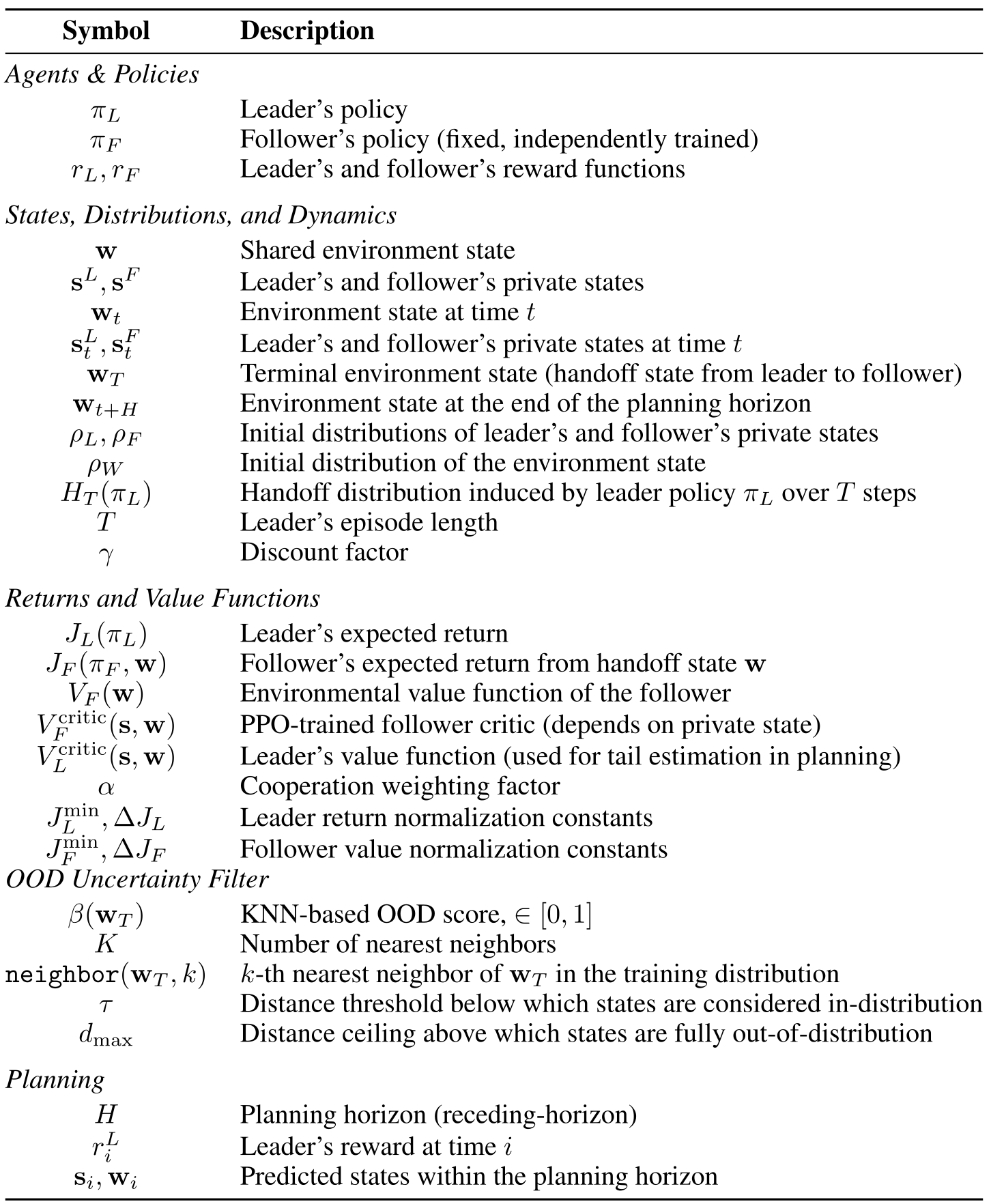
Accessible table, original values and mathematical notation
| Symbol | Description |
| Agents & Policies | |
| Leader’s policy | |
| Follower’s policy (fixed, independently trained) | |
| Leader’s and follower’s reward functions | |
| States, Distributions, and Dynamics | |
| Shared environment state | |
| Leader’s and follower’s private states | |
| Environment state at time | |
| Leader’s and follower’s private states at time | |
| Terminal environment state (handoff state from leader to follower) | |
| Environment state at the end of the planning horizon | |
| Initial distributions of leader’s and follower’s private states | |
| Initial distribution of the environment state | |
| Handoff distribution induced by leader policy over steps | |
| Leader’s episode length | |
| Discount factor | |
| Returns and Value Functions | |
| Leader’s expected return | |
| Follower’s expected return from handoff state | |
| Environmental value function of the follower | |
| PPO-trained follower critic (depends on private state) | |
| Leader’s value function (used for tail estimation in planning) | |
| Cooperation weighting factor | |
| Leader return normalization constants | |
| Follower value normalization constants | |
| OOD Uncertainty Filter | |
| KNN-based OOD score, | |
| Number of nearest neighbors | |
| -th nearest neighbor of in the training distribution | |
| Distance threshold below which states are considered in-distribution | |
| Distance ceiling above which states are fully out-of-distribution | |
| Planning | |
| Planning horizon (receding-horizon) | |
| Leader’s reward at time | |
| Predicted states within the planning horizon | |
Appendix B Extended Related Work
The extended comparison positions direct one-shot preference exchange between jointly learned communication, fixed robust strategies and environment co-design. Its claims describe the cited formulations, without establishing that all methods in those broader research areas are incompatible with sequential tasks.
Ad Hoc Teamwork
PLASTIC and TEAMSTER infer teammate/environment behavior from experience; this interface explicitly transmits preferences and permits distinct tasks. The contrast depends on these particular assumptions, rather than proving a universal separation of ad hoc teamwork and communication.
Zero Shot Coordination
Other-Play learns fixed robust strategies; PAVE instead adapts online to a communicated value interface. Thus its lack of joint training should not be conflated with an absence of test-time adaptation.
Multi-Agent Reinforcement Learning and Shared Critics
Centralized/decentralized training and execution address simultaneous interactions and shared critics in different ways. PAVE studies whole-episode handoffs between separately trained embodiments and keeps the follower fixed. Consecutive-policy work informs the finetuning control, but its original setting and training procedure differ.
Stigmergy
Stigmergy coordinates through environmental traces; PAVE communicates value explicitly, then modifies the physical environment. The source’s broad claim that animal paths provably converge to optimal solutions is stronger than needed here; no such universal convergence claim is adopted for PAVE.
Environmental Co-Optimization
Environment co-design directly optimizes layout and policies. Here the environment changes only through the leader’s feasible actions and the follower does not relearn. That action-mediated restriction is central to the handoff problem.
Sampling-Based Model Predictive Control with Learned Cost Functions
The online search is sampling-based MPC with CEM and learned-value bootstrapping; those components are established. The specific contribution is using a separate follower’s environmental value/support as a coordination interface. KNN attenuation is heuristic coverage filtering, without a bound on extrapolation error.
Original mathematical definition and qualification
PAVE uses a sampling-based MPC formulation [34] with the Cross-Entropy Method [27] as the inner optimizer, similar to its use in model-based RL planners such as PETS [3]; recent CEM variants such as iCEM [23] are complementary and could be incorporated. For tail estimation, PAVE bootstraps the leader’s return using its own value function , following standard practice in value-augmented MPC [21, 13]. The general principle of pairing a search procedure with a learned value estimate was demonstrated at scale by AlphaGo Zero [30], which used a learned value function to evaluate leaf nodes within Monte Carlo Tree Search. The role of the follower’s value function differs as it serves as the coordination interface through which the two independently trained agents communicate their preferences. PAVE additionally employs a -nearest-neighbor distance-based Out-Of-Distribution detector [32, 35] to down-weight the value-function term in environment state regions in which the follower critic has not been trained to prevent inaccurate value approximations.
Learned Communication
One-shot exchange has a predefined semantic meaning instead of a channel learned between jointly trained partners. The transmitted object is a callable value/support representation, not one scalar handoff score. Compatible coordinates and access to an uncertainty computation still constrain arbitrary pairing; message size/communication cost are not measured.
Appendix C Simulation Environments
All simulation environments are custom NumPy implementations. The preserved tables report every reward/penalty. These simplified dynamics and proximity-based pickup/placement conditions differ substantially from contact-rich manipulation.
C.1 Mobile Arm
A base-navigation leader terminates near an object, then a four-degree-of-freedom arm picks/places it automatically when the end effector comes sufficiently close. The follower’s reachable cone depends on base orientation. Zero collision penalty is preserved in the reported follower reward table; success here is not a detailed grasp-physics evaluation.
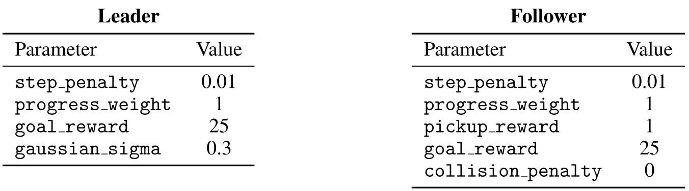
Accessible table, original values and mathematical notation
Leader
| Parameter | Value |
| step_penalty | 0.01 |
| progress_weight | 1 |
| goal_reward | 25 |
| gaussian_sigma | 0.3 |
Follower
| Parameter | Value |
| step_penalty | 0.01 |
| progress_weight | 1 |
| pickup_reward | 1 |
| goal_reward | 25 |
| collision_penalty | 0 |
C.2 Obstacle Arena
The leader clears the lower arena by pushing an obstacle to a wall; the follower traverses a bottleneck. A selfish push can block the only passage. All reward weights remain, including the follower’s large collision penalty300 and shaping terms.
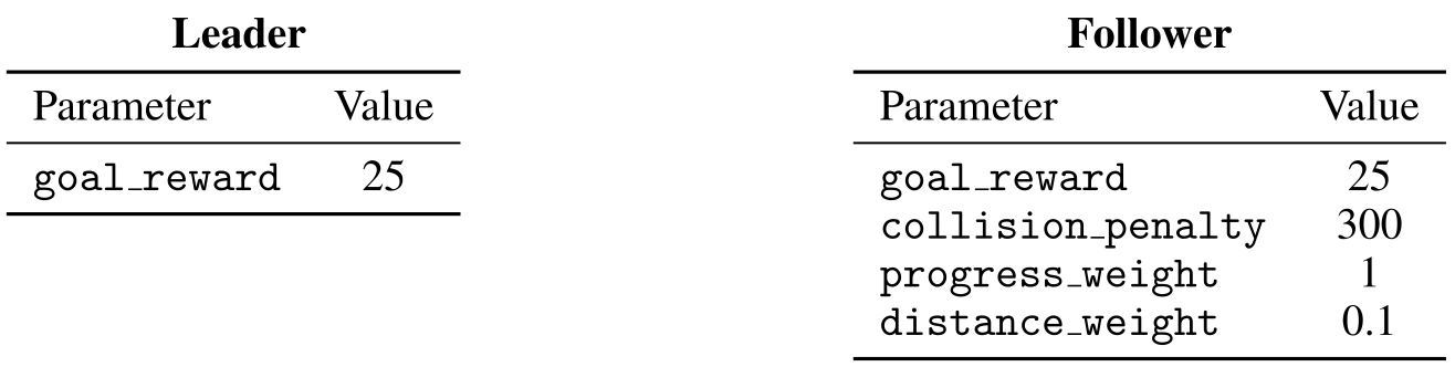
Accessible table, original values and mathematical notation
Leader
| Parameter | Value |
| goal_reward | 25 |
Follower
| Parameter | Value |
| goal_reward | 25 |
| collision_penalty | 300 |
| progress_weight | 1 |
| distance_weight | 0.1 |
C.3 WAREHOUSE Family
The warehouse leader selects among three transfer areas; the follower retrieves and shelves the object. Pickup/placement occur by proximity and orientation. Blocked removes center pickup capability; Unseen permits it physically but omits center training experience. Capability limits and training-support limits are different, even though a critic can overestimate both.
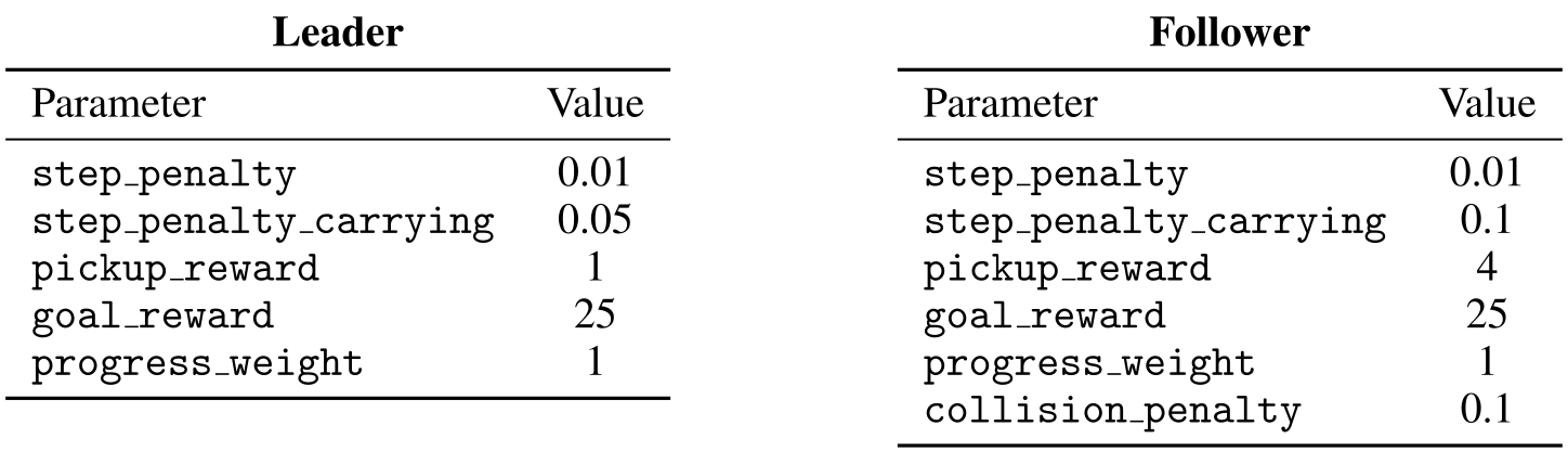
Accessible table, original values and mathematical notation
Leader
| Parameter | Value |
| step_penalty | 0.01 |
| step_penalty_carrying | 0.05 |
| pickup_reward | 1 |
| goal_reward | 25 |
| progress_weight | 1 |
Follower
| Parameter | Value |
| step_penalty | 0.01 |
| step_penalty_carrying | 0.1 |
| pickup_reward | 4 |
| goal_reward | 25 |
| progress_weight | 1 |
| collision_penalty | 0.1 |
C.4 HOUSEHOLD
Household changes the leader objective to reaching virtual dirt beneath a box representing a table, rather than pushing the obstacle to a wall. The exact simulation reward table remains. The physical demonstration does not clean real dust or manipulate a full household table.
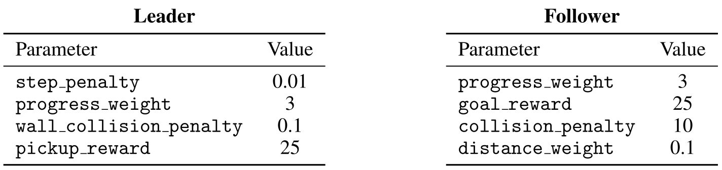
Accessible table, original values and mathematical notation
Leader
| Parameter | Value |
| step_penalty | 0.01 |
| progress_weight | 3 |
| wall_collision_penalty | 0.1 |
| pickup_reward | 25 |
Follower
| Parameter | Value |
| progress_weight | 3 |
| goal_reward | 25 |
| collision_penalty | 10 |
| distance_weight | 0.1 |
Appendix D Training and Model Selection
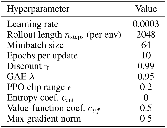
Independent Gaussian MLP policies use two 64-unit hidden layers and the retained PPO hyperparameters/budgets. Runs with below 70% individual success are discarded uniformly before comparing methods, so the six-seed results condition on competent policies. This is not selection on PAVE’s final score, but excludes weak agents. Finetuning receives 1.5M additional steps and alpha one because it outperformed alpha four; PAVE uses four. Exact budgets and selection details remain available.
Original mathematical definition and qualification
Table 2 was generated by evaluating our method and the baseline over six independent training and evaluation seeds. PAVE assumes capable actors, so we discard policies with under individual success. Applied uniformly across all baselines, this ensures a fair cross-method comparison. This removes noise from followers that fail regardless of interaction method while preserving variance among competent policies. No further selection of seeds was performed based on the performance of our method or baselines.
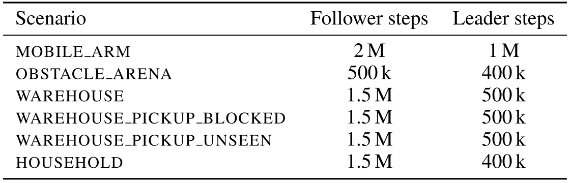
Accessible table, original values and mathematical notation
| Scenario | Follower steps | Leader steps |
| mobile_arm | 2 M | 1 M |
| obstacle_arena | 500 k | 400 k |
| warehouse | 1.5 M | 500 k |
| warehouse_pickup_blocked | 1.5 M | 500 k |
| warehouse_pickup_unseen | 1.5 M | 500 k |
| household | 1.5 M | 400 k |
Original mathematical definition and qualification
All Finetuning experiments were run for an additional 1.5M steps. The return signal is computed as the sum of the normalized leader return and the normalized follower return, with the latter scaled by . This differs from the used in PAVE. We made this choice because Finetuning with yielded higher success rates than with , so we report only the best-performing version of the Finetuning baseline.
Appendix E Hardware Setup
Two RoboMasters and the box are tracked by OptiTrack, with velocity control and pose feedback at 50 Hz. Policies transfer from simulation; PAVE plans with the same nominal model. This is controlled motion-capture deployment with virtual dirt, rather than onboard visual scene inference. Fifty hertz is low-level feedback/control; the paper does not report CEM wall-clock planning latency or certify it meets every update deadline.
Trials
Both Naive and PAVE run each of twenty randomized initial configurations, allowing paired comparison. Box orientation and robot starts vary within the designated halves. The reported 30/70% follower rates correspond to 6/14 successes; no unreported number of independent setups or training seeds is inferred.
Sim-To-Real Transfer and Failure Modes
Simple velocity matching omits much physical friction/contact behavior. Replanning can compensate empirically, but real leaders often require repeated pushes after slips or under-rotation. Selected successful videos illustrate that mechanism without proving a bound on model mismatch or all-trial robustness.
Appendix F Planner Details
CEM initializes action means from a policy rollout and fits Gaussian elites with a variance floor. Alpha 4, gamma .99 and return ranges from 200 prior episodes are shared. Horizons/samples/iterations vary by scenario: Mobile 30/200/4, Obstacle 40/300/10, warehouse variants 40/500/10, Household 20/100/5; replanning is every 3 or 5 steps. Sigma-noise is called covariance in prose while the table also gives minimum standard deviation; the exact source naming is retained rather than silently resolving its units. No timing table establishes planner compute cost.
Original mathematical definition and qualification
The CEM planner uses a Gaussian action distribution with elite selection. We warm-start the action distributions by setting the mean to the actions obtained from rolling out the naive leader policy through the dynamics, and we initialize the covariance to . At each iteration, we draw samples from the action distribution and evaluate them with respect to the objective defined in Equation (5). We then select the best samples and update the action distribution by fitting a Gaussian to them. To prevent covariance collapse, we impose a lower bound on the covariance.
Original mathematical definition and qualification
We instantiate the cost using the same parameters and procedures across all scenarios. Specifically, we use a follower value weighting term of , a discount factor of , and normalize the leader and follower returns to using the returns from 200 rollout episodes of the prior policies.

Accessible table, original values and mathematical notation
| Scenario | Horizon | Samples | Iters | Elite frac. | Min. std | Replan | Dist. | |
| mobile_arm | 30 | 200 | 4 | 0.2 | 0.5 | 0.1 | 5 | gaussian |
| obstacle_arena | 40 | 300 | 10 | 0.3 | 0.5 | 0.208 | 3 | gaussian |
| warehouse | 40 | 500 | 10 | 0.2 | 1.5 | 0.1 | 5 | gaussian |
| warehouse_pickup_blocked | 40 | 500 | 10 | 0.2 | 1.5 | 0.1 | 5 | gaussian |
| warehouse_pickup_unseen | 40 | 500 | 10 | 0.2 | 1.5 | 0.1 | 5 | gaussian |
| household | 20 | 100 | 5 | 0.3 | 0.5 | 0.2 | 5 | gaussian |
Appendix G Case Study: Value Function and Uncertainty Estimate
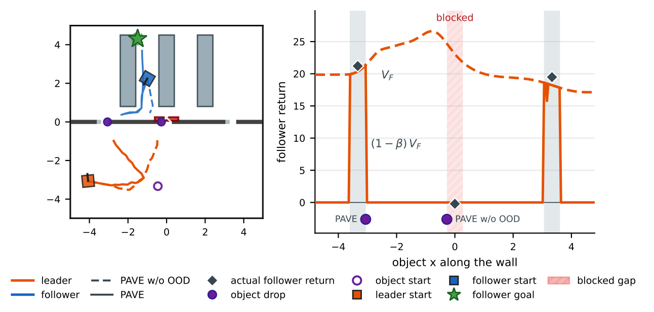
The complete case study shows overoptimistic center/drop-off values and the attenuated curve, all paths/legends and actual follower returns. It illustrates one blocked warehouse example. Density filtering helps there, while the main ablation shows it can reduce performance elsewhere.
Appendix H Decomposition of the Leader Objective
The full mathematical argument is retained. Relative to a globally selfish-optimal policy, cooperative gain equals alpha times follower improvement minus leader loss; improvement requires the former to exceed the latter. If the selfish policy also maximizes follower return over all feasible leaders, it is already cooperative-optimal. This is an exact algebraic statement about ideal policies/returns, not a convergence theorem for CEM, a guarantee that a learned Naive policy is optimal, or a constraint preventing leader sacrifice. It does not by itself establish recursive multi-agent baseline preservation.
Original mathematical definition and qualification
In this section, we call a leader policy selfish if it optimizes only the leader’s individual objective, without regard to the follower. Formally, given a feasible leader policy class , a selfish leader policy is any
Equation
Original mathematical definition and qualification
For a cooperation weight , we define the cooperative objective
Equation
Original mathematical definition and qualification
We call a leader policy -optimal if it maximizes over . For any alternative leader policy , the improvement over the selfish leader decomposes as
Equation
Original mathematical definition and qualification
Consequently, for , adapting the leader can improve the cooperative objective exactly when the induced follower gain exceeds the leader loss scaled by :
Equation
Original mathematical definition and qualification
For , the cooperative objective reduces to the selfish leader objective, so any selfish leader’s policy is already optimal.
Equation
Original mathematical definition and qualification
then no feasible deviation can improve the follower term, while every deviation does not increase the leader term. In that case, the selfish leader is already -optimal for every .
Appendix I Generative AI Usage Disclosure
The authors disclose AI assistance with editing, exploration, figure boilerplate and code generation, with author review and responsibility.
Appendix J Reproducibility Statement
The source links the public code and supplies architecture, training, OOD and planner settings. Manuscript-level gaps remain in some distance/normalization/index conventions and measured compute timing; no uninspected implementation behavior is asserted.