Overview
A data-collection loop that proposes auxiliary robot tasks with a vision-language model, then allocates demonstrations using training-data attribution. All original figures, tables, equations, pseudocode, three complete prompts and the asset/task inventories are retained.
At a glance
GUILD targets a deployment task with few available demonstrations by collecting useful data in other environments. A vision-language model expands the candidate task set; differentiable attribution estimates which existing task data improve a target-data loss and guides the next collection batch. Tests use three simulated and four physical manipulation tasks. Gains support adaptive collection in these settings, while dependence on a small target proxy, proposer feasibility and repeated training limits broader claims.
1 Introduction
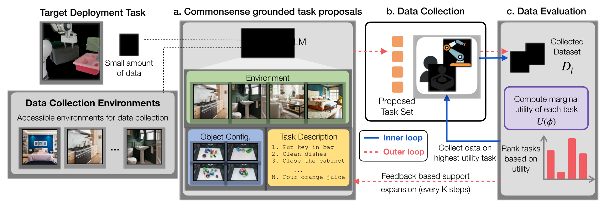
When deployment environments are difficult to access, auxiliary demonstrations can be plentiful yet irrelevant. GUILD treats task choice and demonstration allocation as decisions to update during collection. It starts with a target description/video, accessible scenes/assets and a small target dataset, then alternates broad task proposals with measured training influence. Target demonstrations both define the attribution proxy and participate in policy training; the method is not target-data-free.
2 Related Work
The work combines task-conditioned generation, data selection and predictive attribution. STRAP retrieves visually similar robot sub-trajectories; factored scaling curves predict returns to additional task data. GUILD instead uses MAGIC metagradients to estimate the local effect of reweighting training trajectories, then feeds task rankings back to the proposer. This connects collection to the current learner, rather than assuming visual or semantic similarity alone predicts transfer.
3 Preliminaries
A task parameter ϕ specifies an accessible scene, objects and manipulation objective, and a generator or teleoperator produces trajectories for that parameter. The objective is to choose a collection distribution that maximizes a trained policy’s deployment performance under a demonstration budget. Because physical success is expensive to measure repeatedly, the algorithm substitutes a differentiable loss on the small target dataset. That proxy introduces both approximation error and dependence on target-data coverage.
Equations 1
| (1) |
4 GUILD: Guided Iterative Imitation Learning Data Collection
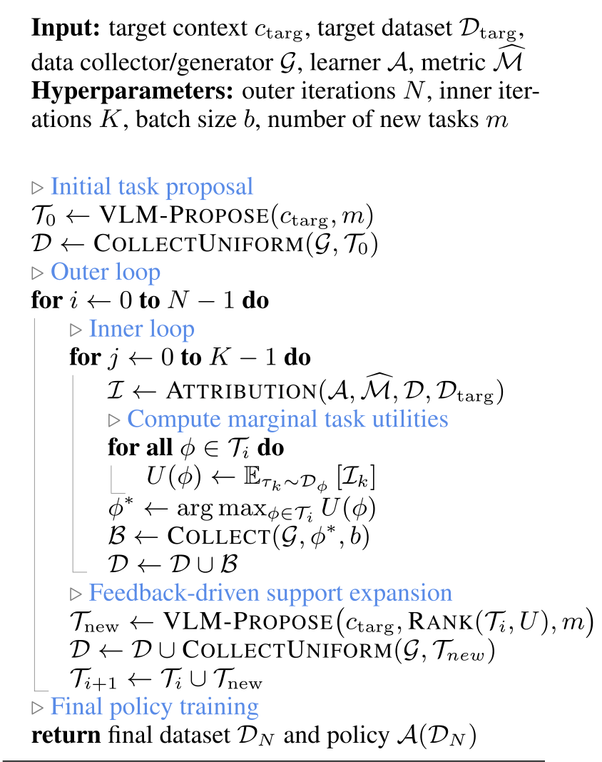
GUILD has an outer loop that expands the discrete task support and an inner loop that chooses where to collect the next batch. Every newly proposed task receives seed demonstrations before attribution can assess it. The final policy trains on accumulated auxiliary data together with the available target demonstrations.
4.1 Task-Parameter-Space Exploration via Commonsense-Grounded Proposals
A vision-language model receives deployment video frames and a language goal plus accessible scenes, objects and placement constraints. It proposes feasible tasks with potentially transferable skills. Later expansions include a ranking of prior tasks by utility and prohibit duplicates. This uses a model prior to search a large space; it does not prove that proposed tasks are executable or informative.
Initialization.
Initial tasks come from the deployment/environment context alone and receive uniform seed data. During later expansion, feedback-based proposals exploit successful task patterns, while context-only proposals preserve exploration. Newly added tasks again receive uniform seeds, so expanding the support has an explicit data cost.
4.2 Data Evaluation via Predictive Attribution
Linearize target performance with respect to trajectory weights around the current dataset. MAGIC differentiates through the policy-training computation to obtain trajectory metagradients; mean attribution within each task estimates its marginal utility. Collect a small batch for the best task, retrain/recompute, and repeat as returns change. The main text substitutes validation loss into a maximization formulation, while Appendix C.3 treats positive loss utility as undesirable; the ranking must therefore use a consistent loss-reduction direction. The originals retain this unresolved sign convention. Local reweighting sensitivity is an approximation to the benefit of new demonstrations, not a guaranteed causal effect.
Equations 2–4
| (2) |
| (3) |
| (4) |
5 Experiments
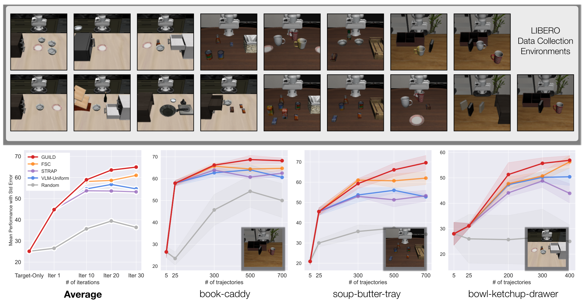
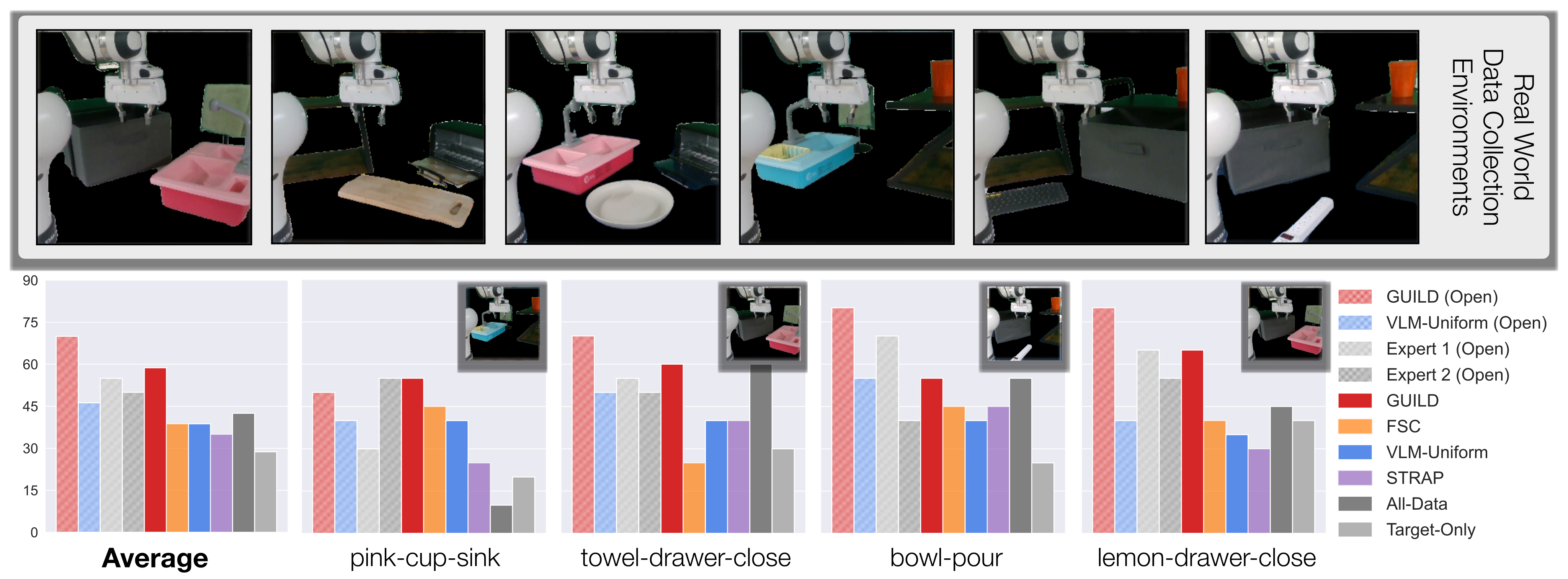
The study compares task selection under matched collection budgets in LIBERO simulation and physical manipulation. Baselines include uniform collection over model-proposed tasks, random simulation tasks, STRAP and adapted factored scaling curves. Physical experiments distinguish a fixed offline task pool from open-world proposals followed by new teleoperation. The full-pool All-Data baseline additionally includes the target scene, so it is not an equal-access, equal-budget control.
5.1 Results
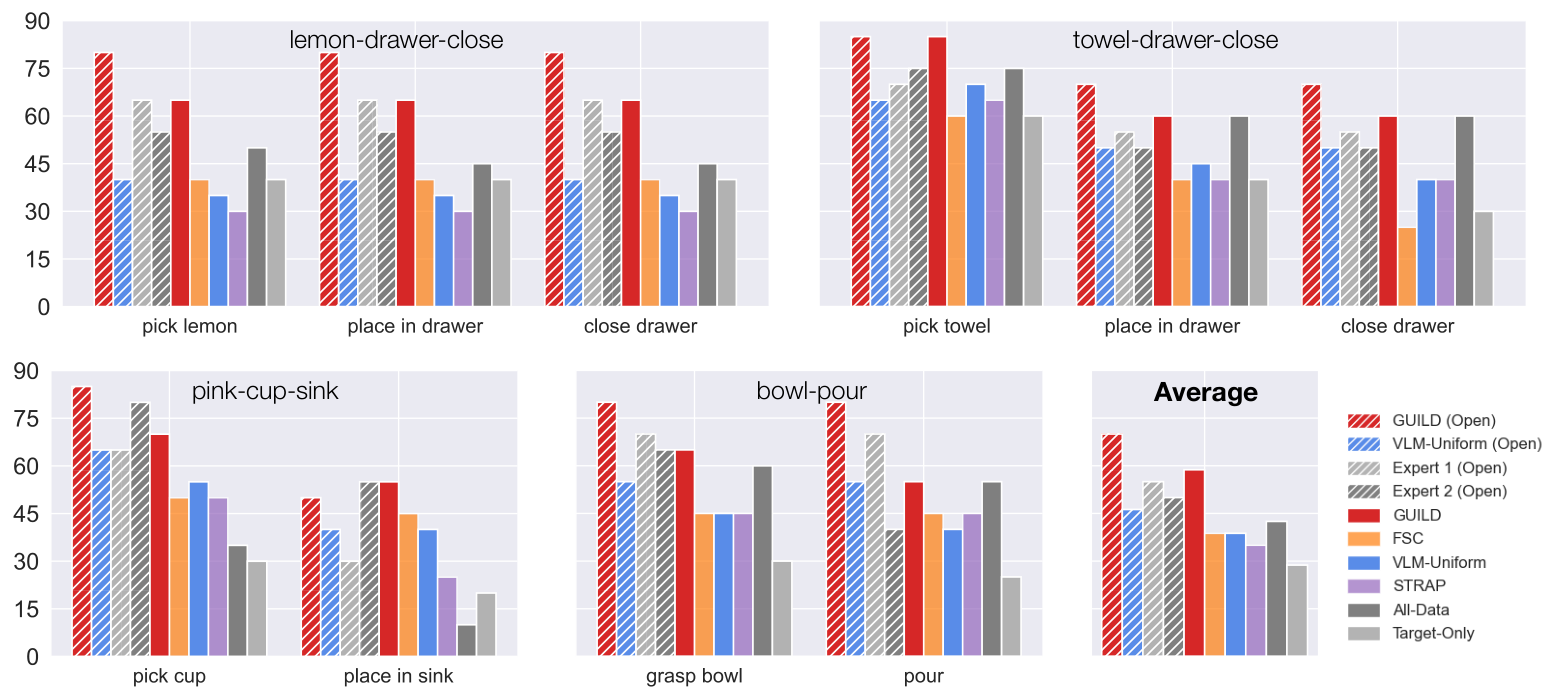
On the three simulated targets, final GUILD success averages 64.9%, with 68.2% book-caddy, 69.6% soup-butter-tray and 56.9% bowl-ketchup-drawer. Figure 2 shows the collection curves and variation across three collection seeds. In the four physical tasks, GUILD leads the plotted budget-matched baselines; open-world comparisons include uniform model proposals and two experts, whereas STRAP/scaling-curve results are restricted to the closed pool. Physical results use 20 common initial configurations per task and do not report multi-seed collection uncertainty. Human comparisons also differ in feedback access: people do not receive GUILD’s iterative attribution outcomes.




5.2 Qualitative Analysis: What Data Does GUILD Collect?
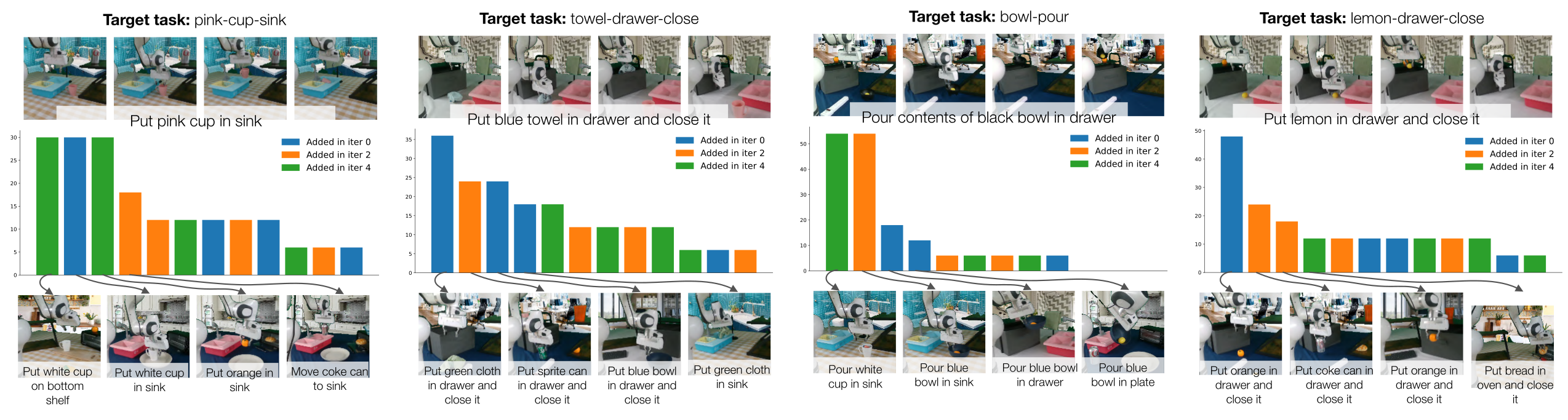
Final allocation is task-specific rather than uniformly spread. The qualitative panels show both when candidate tasks were introduced and how many demonstrations they ultimately received; these distributions illustrate the selection mechanism without independently establishing each task’s causal contribution.
Useful tasks are discovered throughout the collection process.
Some high-allocation auxiliary tasks appear only after later support expansions, indicating that an initial proposal set can miss useful data sources. Attribution feedback can redirect subsequent proposals, although a later task’s allocation alone is not proof that its addition caused the final improvement.
Nature of the final data composition.
Bowl pouring and lemon drawer manipulation concentrate data on a few related tasks, while cup placement and towel manipulation spread it more broadly. Scene, object and motion similarity matter differently for each target. The loop adapts allocation instead of imposing the same diversity level on every task.
6 Conclusion and Limitations
The results favor coupling model-guided exploration with learner-dependent allocation in the tested settings. Limitations include infeasible or repetitive proposals needing human oversight, the cost of repeated training/attribution, and a discrete task representation. Continuous parameter optimization and broader environments remain future work. A small, repeatedly used target dataset may also give an incomplete proxy for deployment success.
Acknowledgments
The authors acknowledge research support, compute resources and colleagues’ assistance. These acknowledgments do not add experimental evidence or alter the evaluation protocol.
Appendix A Method Details
The method appendix gives the support-expansion schedule, differentiable attribution computation and an empirical check of utility as a predictor. These details distinguish the algorithm’s local training surrogate from its final rollout evaluation.
A.1 VLM Task Proposer
GPT-5.2 proposes tasks. Simulation expands after inner iterations 2, 4, 8 and 16, adding five tasks per expansion; expansion i uses i feedback-guided proposals and the rest context-only. Physical experiments expand after iterations 3 and 9, with four new tasks except three for bowl pouring, and use i+1 feedback-guided proposals. All new tasks receive five seed demonstrations in simulation or six physically. This mixture explicitly preserves exploration rather than feeding back rankings for every proposal.
A.2 Data Attribution – Computing Metagradients
MAGIC computes derivatives of target loss through an unrolled training computation. REPLAY checkpoints and re-executes intermediate states to reduce memory use, avoiding storage of the entire trajectory. Metagradients are exact for the chosen differentiable computation, but the finite/truncated training horizon and first-order approximation to new data remain limitations. Task utility averages the trajectory-level scores; recomputing after each batch responds to changing data returns.
Equation
A.2.1 Relationship between Utility and Downstream Performance
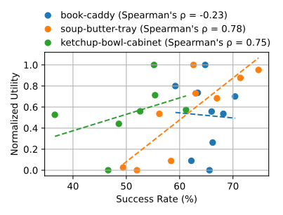
Across datasets produced by the compared strategies, mean utility correlates with final performance at about 0.75 for bowl/ketchup and 0.78 for soup/butter, but −0.23 for book/caddy. The authors suggest that book performance occupies a narrow range. Thus the check is mixed evidence for the proxy, not a universal positive association or an independent guarantee of improvement.
Appendix B Training and Evaluation Details
Training mixes target and auxiliary data equally. Evaluation is separated from the attribution loss by executing trained policies, but the target demonstration set used for attribution is also part of training. Hyperparameter and task-space tables preserve all settings.
| No. of | No. of | No. of Data | Outer-loop | No. of tasks | Batch size | No. of Initial | |
| Training Envs | Target Demos | Collection Iter. | Schedule | Every Iter. () | () | Task Demos | |
| LIBERO | |||||||
| Book-Caddy | 16 | 3 | 30 | [2,4,8,16] | 5 | 20 | 5 |
| Soup-butter-tray | 16 | 5 | 30 | [2,4,8,16] | 5 | 20 | 5 |
| Bowl-ketchup-drawer | 16 | 5 | 30 | [2,4,8,16] | 5 | 10 | 5 |
| Real World | |||||||
| pink-cup-sink | 5 | 15 | 20 | [3, 9] | 4 | 6 | 6 |
| towel-drawer-close | 5 | 30 | 20 | [3, 9] | 4 | 6 | 6 |
| bowl-pour | 5 | 20 | 20 | [3, 9] | 3 | 6 | 6 |
| lemon-drawer-close | 5 | 50 | 20 | [3, 9] | 4 | 6 | 6 |
B.1 LIBERO
LIBERO supplies 17 scenes: hold out the target scene and collect in the other 16. Task parameters choose scene, pick object and placement region, with a null region for pick-only tasks. Scripted collection supplies demonstrations; targets have three book-caddy demonstrations and five each for the other two tasks. Fine-tune Octo-Small for 10,000 steps with a 50/50 target–auxiliary mixture. Each data point averages five trained policies evaluated over 100 rollouts each; the plotted mean and standard error use three independent collection seeds. Collection lasts 30 inner iterations, with batches of 20 for book/soup and 10 for bowl, in addition to task-introduction seeds.
Equation

B.2 Real World
Six constructed physical scenes vary fixtures, tablecloths and replaced green-screen backgrounds, with pose variation and one to three distractors. The target scene is excluded from auxiliary collection; open-world proposals also exclude the target object from the movable-asset list. The four targets use 15 cup, 30 towel, 20 pouring and 50 lemon demonstrations. Fine-tune Octo for 25,000 steps with equal target/auxiliary sampling; evaluate on the same 20 initial configurations across methods. There are 20 collection iterations of six demonstrations plus seed collection. Closed-world selection uses an existing task pool; open-world collection executes newly proposed configurations by teleoperation. The prose says 49 pool tasks, while the original Appendix G table contains 51 task rows; both are preserved.
Equation
B.3 Human Experiment Details
Eight simulation participants have one to more than five years of robotics experience; two physical experts have four to five years. They see the target context, available environments and collection budget, then specify task allocations. They do not receive attribution scores or iterative policy-outcome feedback. The comparison measures these defined workflows, not an equal-feedback test of unrestricted human versus model expertise.
Appendix C Additional Results
Additional analyses retain task allocations, participant-level comparisons, sampling/feedback/model ablations and stage-wise physical failures. Each supports a narrower claim than the overall aggregate success rate.
C.1 Real-World Qualitative Results
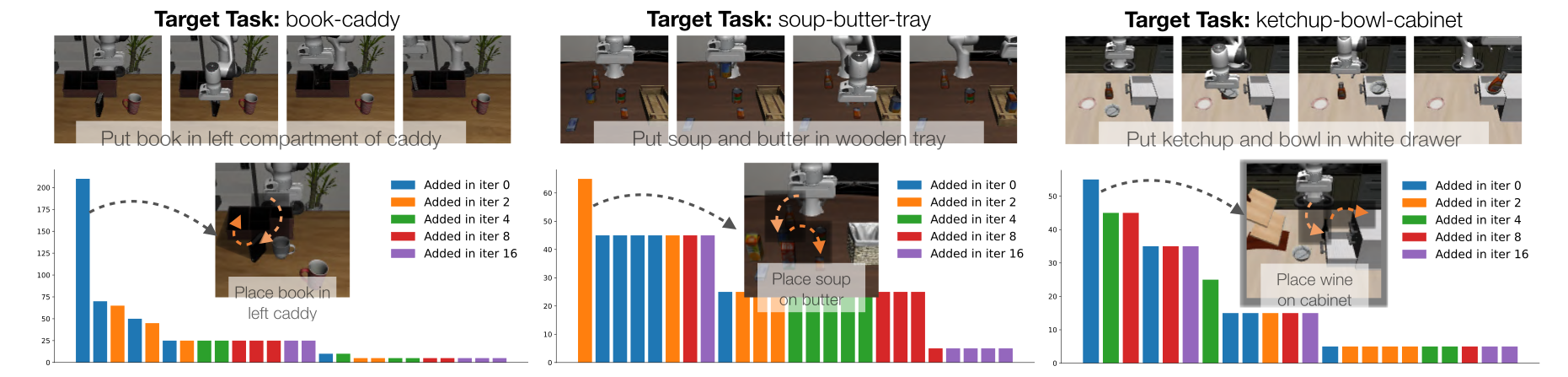
Despite the subsection’s “Real-World” title, Figure 7 shows the three LIBERO targets. Book-caddy data concentrate on a nearly matching left-caddy placement; soup/butter and bowl/ketchup draw on more varied tasks. The caption’s original target naming is retained, including its cabinet/drawer wording variation.
C.2 Human-Guided Data Collection Results
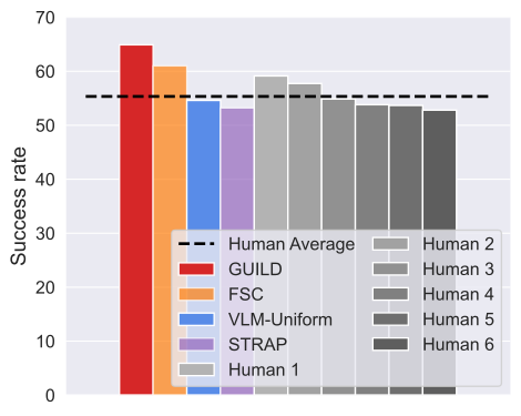
The per-task human comparison shows substantial participant variation, and individual humans can outperform GUILD on a particular task. Averaging the three simulation tasks favors GUILD; uniform model proposals are closer to the average human result. These outcomes retain the feedback-access qualification described in Appendix B.3.
C.3 Hard vs. Soft Sampling
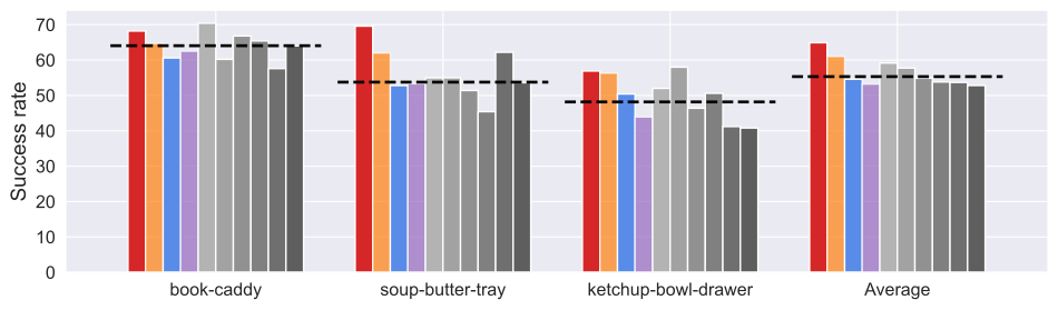
Soft sampling normalizes useful task scores into probabilities rather than assigning the whole batch to the top task. The implementation discussion excludes positive loss-utility values, reinforcing that lower target loss is the desired direction. Hard allocation averages 64.9% versus 61.3% for soft sampling across three simulated targets; task-wise errors overlap in places. Frequent recomputation and continued support expansion partly counter the risk of overconcentrating data.
Equations
| Tasks | book-caddy | soup-butter-tray | bowl-ketchup-drawer | Average |
|---|---|---|---|---|
| GUILD | ||||
| GUILD (soft-sampling) | ||||
| GUILD (no-feedback) | ||||
| GUILD (gemini) |
C.4 Feedback based Support Expansion
Removing ranking feedback lowers the average from 64.9% to 59.2%, driven especially by soup/butter (69.6%→55.3%, a 14.3 percentage-point difference); bowl performance is unchanged. Using feedback for every expansion proposal also reduces bowl success from 56.9±1.8% to 50.7±2.1%, with little reported difference on the other two tasks. Feedback and context-only exploration therefore play complementary roles in these ablations.
C.5 Impact of the VLM Used
Replacing the proposer with Gemini yields 61.1% average versus 64.9% for the default model. Effects vary: soup/butter drops from 69.6% to 52.2%, while bowl rises from 56.9% to 63.8%. This suggests sensitivity to proposal quality and task context, rather than a universal ordering of model families.
C.6 Stage-wise results for Real world tasks
Stage-wise rates are absolute fractions of 20 trials: earlier failures count against every later stage. Grasping is a major bottleneck for bowl and lemon tasks. Cup failures include rim contact, dropping and rack interference; towel failures include deformable placement and recovery. These observations help localize remaining errors but do not supply a separate causal ablation for every failure type.
Appendix D Baseline Implementation
Random/Uniform simulation collection selects feasible tasks and balances demonstration counts. STRAP uses the same model proposal process, DINOv2 visual embeddings and dynamic time warping over trajectory segments; similarity-based weights guide collection and feed outer-loop rankings. The factored-scaling-curve baseline fits four subset sizes per task and uses an offline embedding-similarity adaptation, rather than its full online rollout protocol. With M tasks and four subset sizes it trains 4M policies per step, while GUILD performs one attribution training computation plus replay/metagradients. All-Data uses the full physical pool, including target-scene data, and therefore differs in both volume and access.
Appendix E Metagradient Hyperparameters and Training Cost
The attribution learner uses batch 512, Adam and cosine learning-rate decay. Its nominal training budget C is 500 steps in simulation or 300 physically. The metagradient horizon starts at 50, 75 or 100 steps according to epoch length E, is enlarged to cover at least one epoch, and warmup is min(C−Nₘ,10E). These are the attribution computation’s settings, not differentiation through the full 10,000/25,000-step deployment-policy training.
| Hyperparameter | LIBERO | Real-World |
|---|---|---|
| Policy architecture | Octo-Small | Octo-Small |
| Warmup steps | Adaptive | Adaptive |
| Metagradient steps | Adaptive | Adaptive |
| Max step bound | 500 | 300 |
| Batch size | 512 | 512 |
| Optimizer | Adam | Adam |
| Learning-rate scheduler | Cosine | Cosine |
Equations
Training Cost.
Attribution takes approximately 10–15 minutes on four NVIDIA A5000 GPUs. A data batch takes a few minutes in simulation or 15–30 minutes physically. The reported full process lasts about 7–8 hours for 30 simulated iterations and 10–15 hours for 20 physical iterations. Adaptive collection therefore trades additional compute and scheduling complexity for useful demonstration allocation; the paper does not establish that it minimizes total wall-clock or labor cost.
Appendix F Prompts used for VLM task-proposer
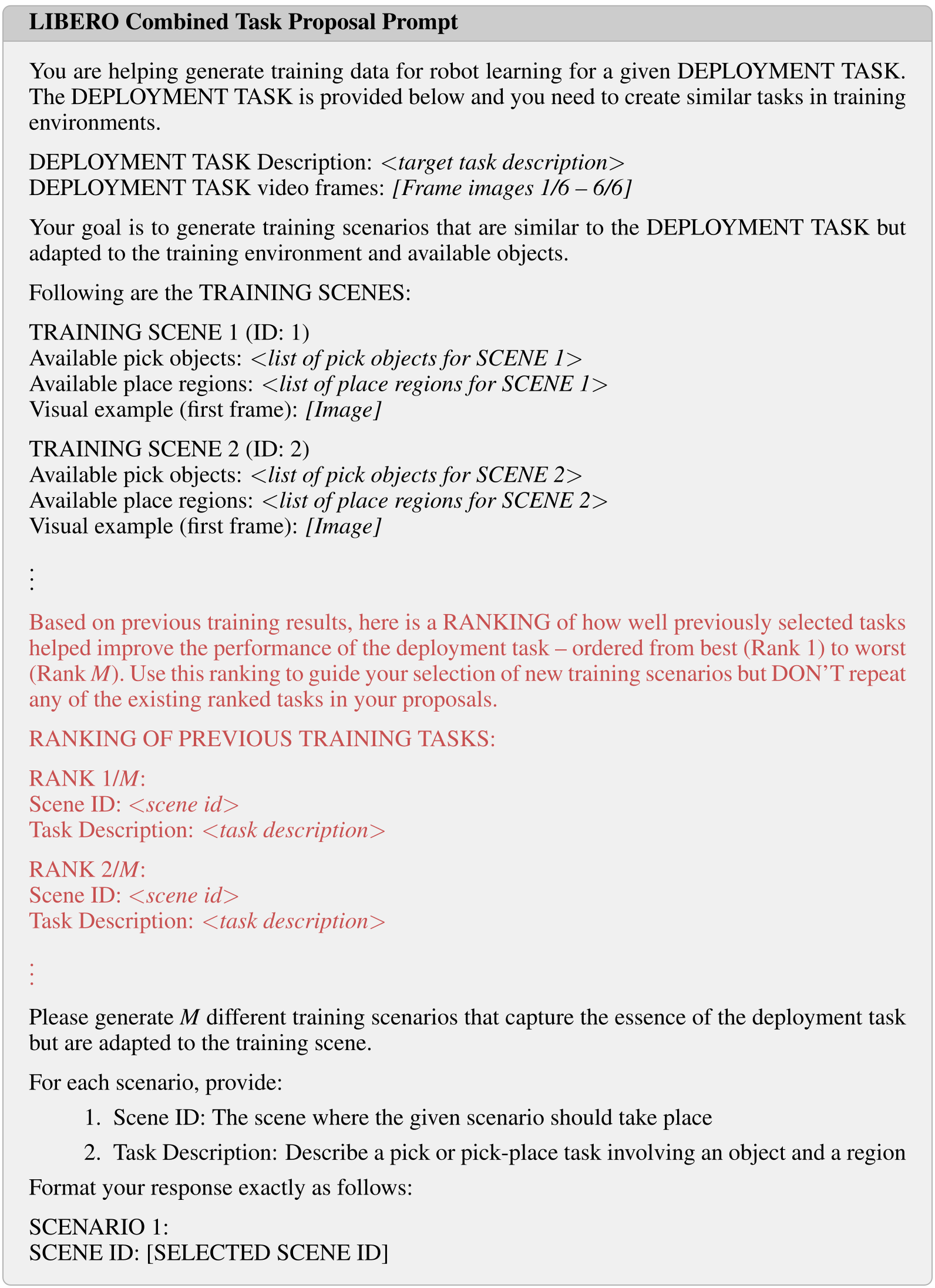
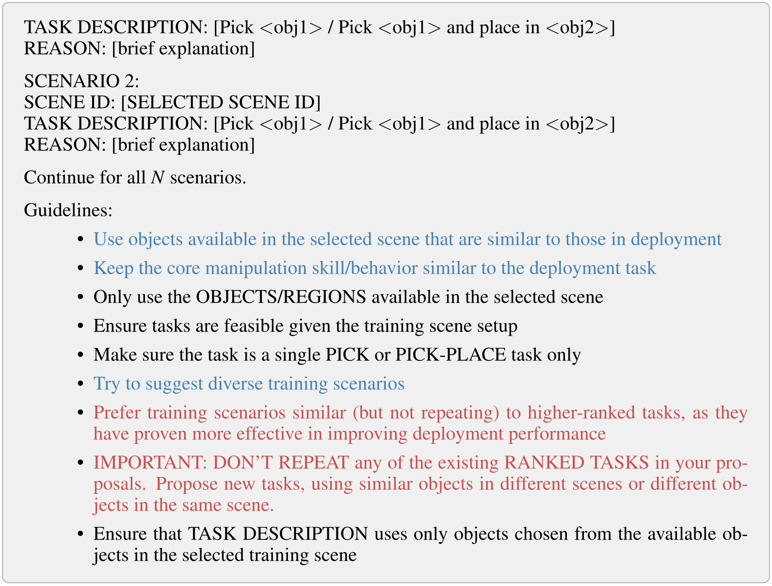
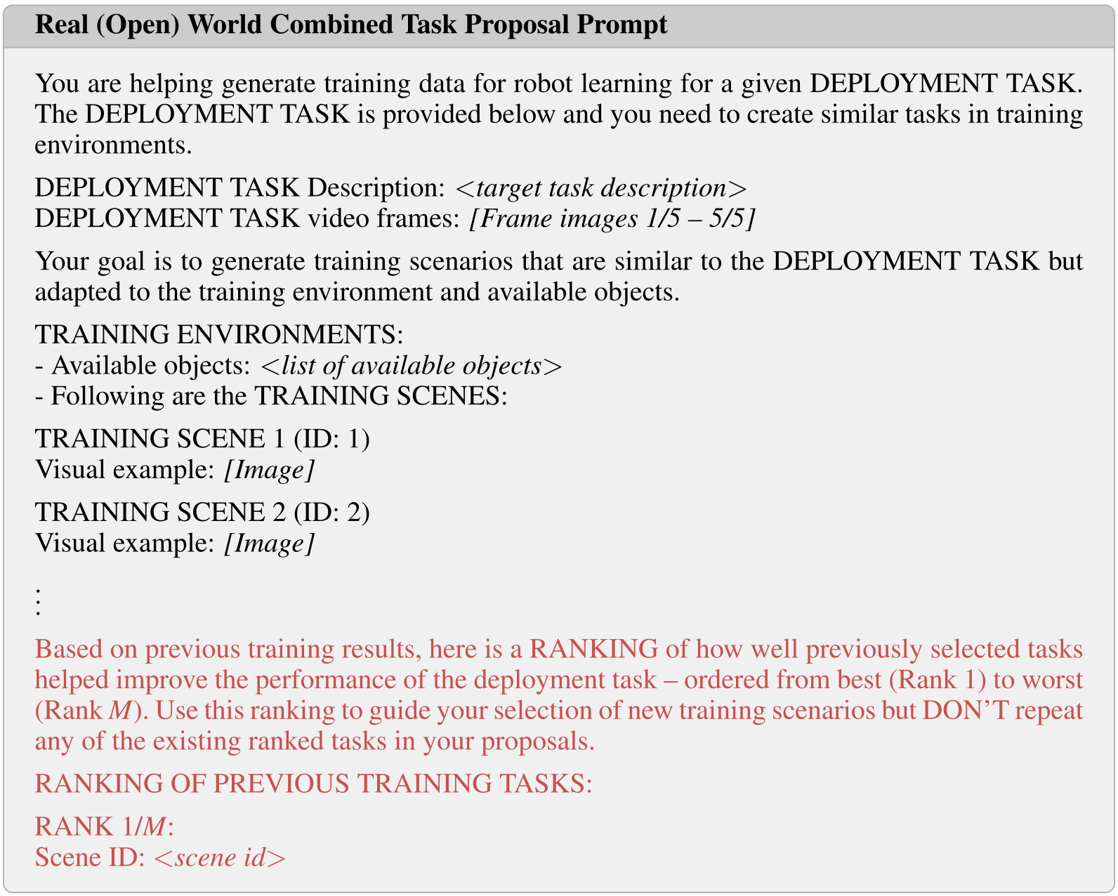
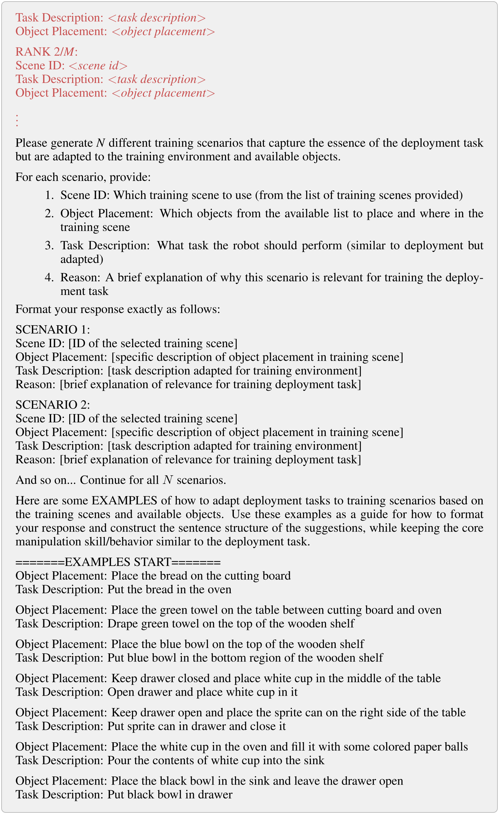
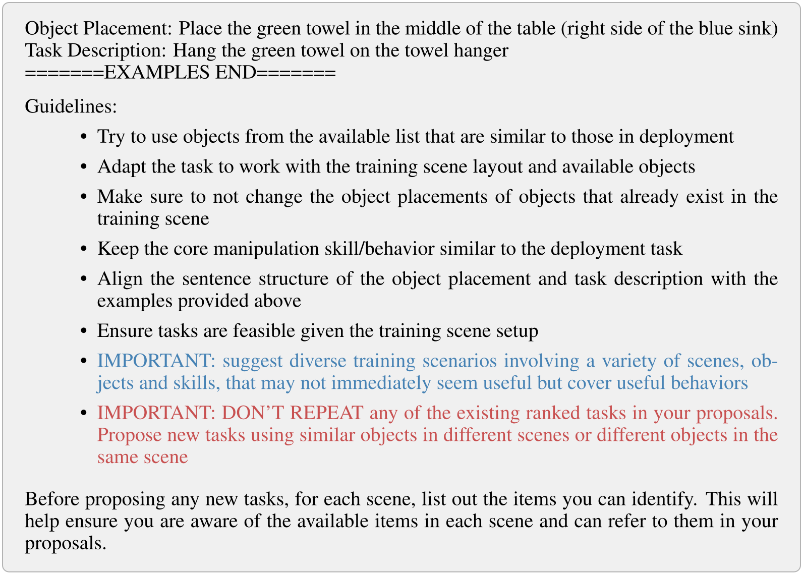
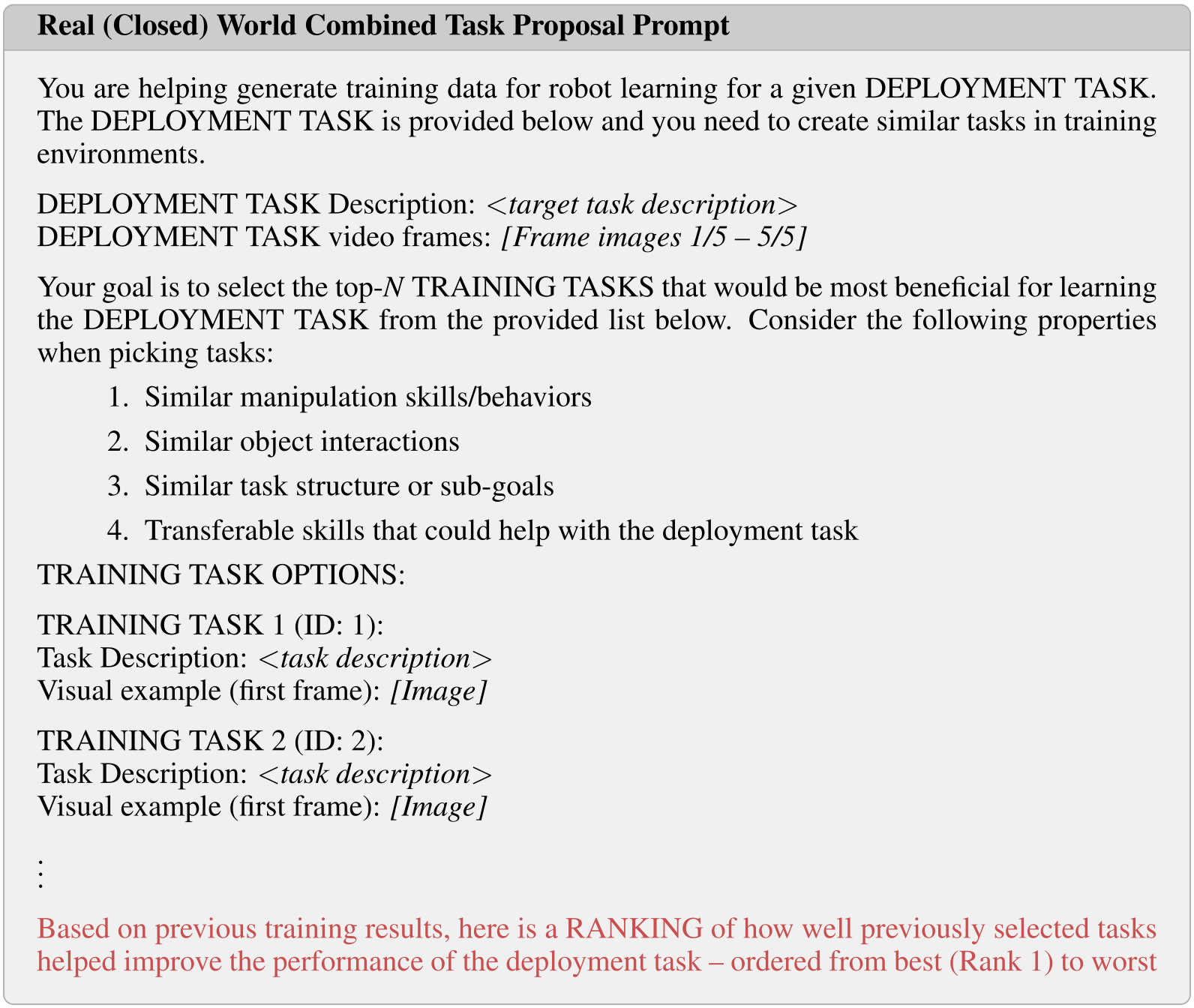
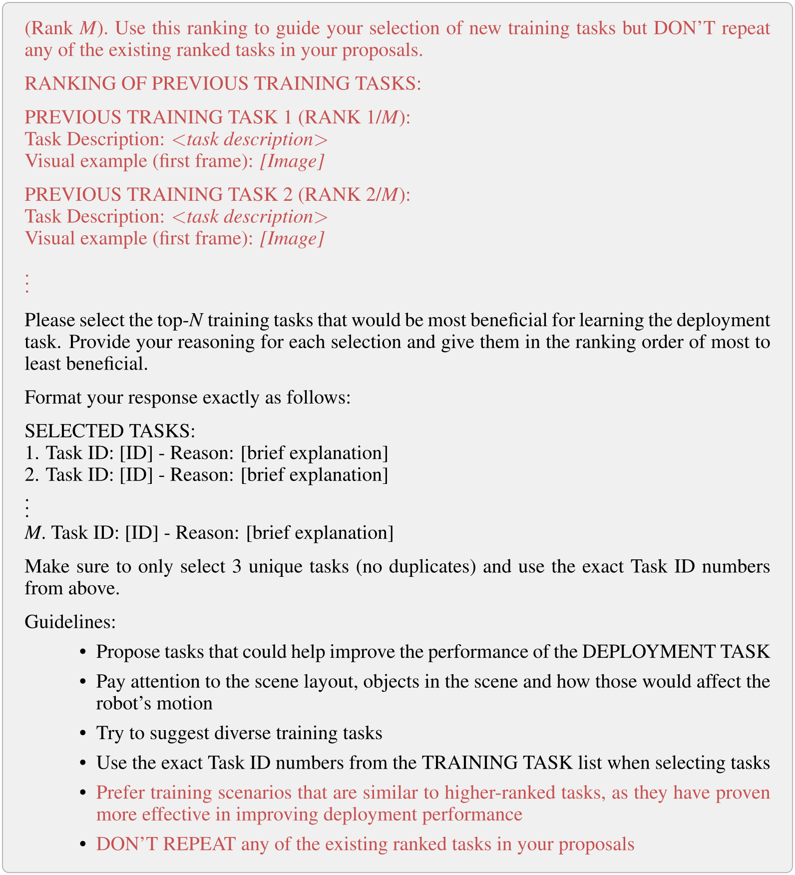
All three original prompts are retained in native PDF form, including colored instructions and every example. Black text is shared, blue applies to initial/context-only proposals, and red introduces ranking feedback. Their placeholders and occasional template inconsistencies remain visible rather than being silently repaired.
F.1 LIBERO
The LIBERO prompt supplies six deployment frames and per-scene pick objects/placement regions. It requests a scene, a feasible single pick or pick-and-place task, and a reason. Feedback ranks earlier tasks and prohibits repetition; context-only instructions emphasize diversity. The original template mixes M and N placeholders, which are preserved.
F.2 Real (Open-World)
The open-world prompt supplies five deployment frames, movable objects and scene images. It requests scene, object placement, task description and justification, with eight complete adaptation examples. Existing fixtures must remain in place, and the model first inventories visible scene items. Initial instructions encourage diverse potentially transferable behaviors; feedback instructions favor related but nonduplicate tasks. All continuation pages are retained.
F.3 Real (Closed-World)
The closed-world prompt ranks existing task IDs rather than generating new configurations. It includes deployment frames, task descriptions/examples and prior utility rankings. Although it uses top-N/M placeholders, one instruction hardcodes three unique tasks; the reported physical schedule uses four for most targets and three for bowl pouring. This template inconsistency is explicitly preserved, and the paper does not explain the exact runtime substitution.
Appendix G Training Environment Assets
The original inventories define which environments, objects and task choices were available to the proposer. Retaining these tables is necessary to assess feasibility and the scope of the collection experiments.
G.1 LIBERO
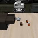
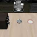
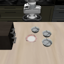
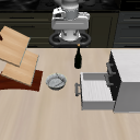
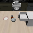
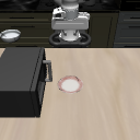
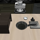
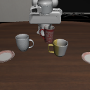
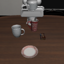
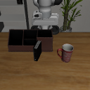
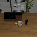
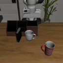
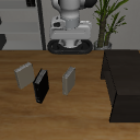
The LIBERO gallery lists all 17 scenes with their pickable objects and valid placement regions. A target uses the other 16 scenes for auxiliary collection. All 17 original 128×128 scene images are retained at native resolution, together with every object and region label.
| Scene Image | Pick Objects | Place Objects |
|---|---|---|
|
akita_black_bowl_1, butter_1, butter_2, chocolate_pudding_1 | wooden_cabinet_1_top_side, wooden_cabinet_1_top_region, akita_black_bowl_1, butter_1, butter_2, chocolate_pudding_1 |
|
akita_black_bowl_1, plate_1 | wooden_cabinet_1_top_side, wooden_cabinet_1_top_region, akita_black_bowl_1, plate_1 |
|
akita_black_bowl_1, akita_black_bowl_2, akita_black_bowl_3, plate_1 | wooden_cabinet_1_top_side, wooden_cabinet_1_top_region, akita_black_bowl_1, akita_black_bowl_2, akita_black_bowl_3, plate_1 |
|
akita_black_bowl_1, wine_bottle_1 | white_cabinet_1_top_side, white_cabinet_1_top_region, white_cabinet_1_bottom_region, wine_rack_1_top_region, akita_black_bowl_1, wine_bottle_1 |
|
akita_black_bowl_1, plate_1, ketchup_1 | white_cabinet_1_top_side, white_cabinet_1_top_region, white_cabinet_1_bottom_region, akita_black_bowl_1, plate_1, ketchup_1 |
|
white_bowl_1, plate_1 | microwave_1_top_side, plate_1 |
|
white_bowl_1 | flat_stove_1_cook_region, wooden_two_layer_shelf_1_top_side, chefmate_8_frypan_1 |
|
alphabet_soup_1, cream_cheese_1, tomato_sauce_1, ketchup_1 | basket_1_contain_region, alphabet_soup_1, cream_cheese_1, tomato_sauce_1, ketchup_1 |
|
alphabet_soup_1, cream_cheese_1, tomato_sauce_1, ketchup_1, orange_juice_1, milk_1, butter_1 | basket_1_contain_region, alphabet_soup_1, cream_cheese_1, tomato_sauce_1, ketchup_1, orange_juice_1, milk_1, butter_1 |
|
alphabet_soup_1, cream_cheese_1, tomato_sauce_1, ketchup_1, butter_1 | wooden_tray_1_contain_region, alphabet_soup_1, cream_cheese_1, tomato_sauce_1, ketchup_1, butter_1 |
|
akita_black_bowl_1, akita_black_bowl_2, chocolate_pudding_1 | wooden_tray_1_contain_region, akita_black_bowl_1, akita_black_bowl_2, new_salad_dressing_1, chocolate_pudding_1 |
|
porcelain_mug_1, red_coffee_mug_1, white_yellow_mug_1, plate_1, plate_2 | living_room_table_plate_left_region, living_room_table_plate_right_region, porcelain_mug_1, red_coffee_mug_1, white_yellow_mug_1, plate_1, plate_2 |
|
porcelain_mug_1, red_coffee_mug_1, plate_1, chocolate_pudding_1 | living_room_table_plate_left_region, living_room_table_plate_right_region, porcelain_mug_1, red_coffee_mug_1, plate_1, chocolate_pudding_1 |
|
black_book_1, red_coffee_mug_1 | desk_caddy_1_right_contain_region, desk_caddy_1_left_contain_region, black_book_1, red_coffee_mug_1 |
|
black_book_1, white_yellow_mug_1 | study_table_desk_caddy_right_region, desk_caddy_1_right_contain_region, desk_caddy_1_left_contain_region, black_book_1, white_yellow_mug_1 |
|
black_book_1, red_coffee_mug_1, porcelain_mug_1 | study_table_desk_caddy_right_region, desk_caddy_1_right_contain_region, desk_caddy_1_left_contain_region, black_book_1, red_coffee_mug_1, porcelain_mug_1 |
|
black_book_1, yellow_book_1, yellow_book_2 | wooden_two_layer_shelf_1_top_side, black_book_1, yellow_book_1, yellow_book_2 |
G.2 Real (Open-World)
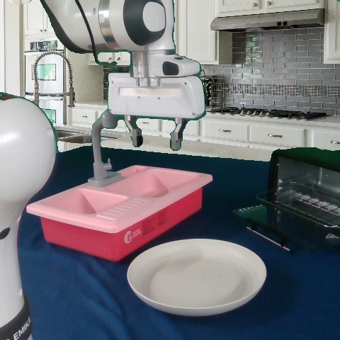
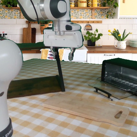
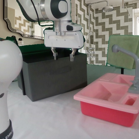
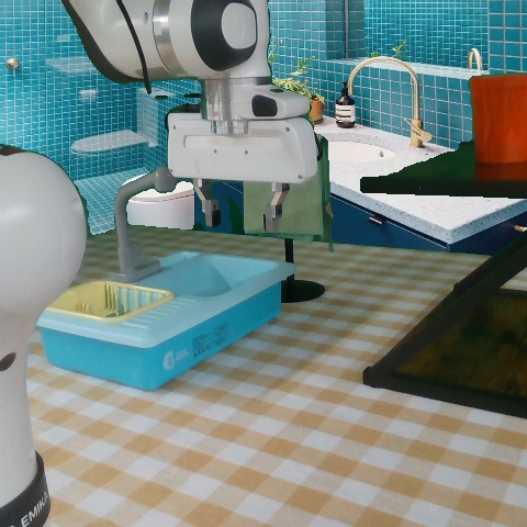
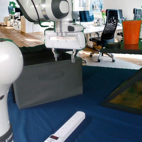
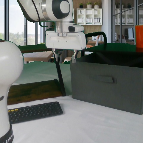
The physical inventory lists available movable objects and six scene photographs, including kitchen, bathroom and office-style configurations. All six original 480×480 photographs and their scene labels are retained. Open-world task proposals must operate within these assets and preserve existing scene fixtures.
| Kitchen 1 (k1) | Kitchen 2 (k2) | Bathroom 1 (b1) | Bathroom 2 (b2) | Office 1 (o1) | Office 2 (o2) |
|---|---|---|---|---|---|
 |
 |
 |
 |
 |
 |
G.3 Real (Closed-World)
The full closed-world task inventory is retained with scene and task text for all 51 body rows. The source prose describes a 49-task pool; the table itself contains 51 listed tasks. This discrepancy is unresolved, so the edition neither drops rows to match the prose nor invents an explanation.
| Scene ID | Initial Object Placement | Task |
|---|---|---|
| k1 | White cup was placed on the plate | Put white cup in the sink |
| k1 | Bread was placed on the plate | Put bread in the oven |
| k1 | Black bowl was placed in the oven | Put black bowl in the sink |
| k1 | Orange was placed on the plate | Put orange in the oven |
| k1 | Coke can was placed in the drying rack | Put coke can on the plate |
| k1 | White cup was placed in the oven and filled with some colored paper balls | Pour the contents of white cup into the sink |
| k1 | Black bowl was placed on the plate and blue bowl was placed in the drying rack | Stack the black bowl on blue bowl |
| k1 | Blue towel was placed in the sink | Put the blue towel next to plate |
| k1 | Orange was placed in the oven | Put orange on plate |
| k2 | Bread was placed on the cutting board | Put the bread in the oven |
| k2 | Lemon was placed on the cutting board | Put the lemon in the oven |
| k2 | Blue bowl was placed in the oven | Put blue bowl in the bottom region of the shelf |
| k2 | Coke can was placed on the cutting board | Put coke can in the bottom region of the shelf |
| k2 | Sprite can was placed in the bottom region of the shelf | Put sprite can on the cutting board |
| k2 | Green towel was placed on the table between cutting board and oven | Drape green towel on the top shelf |
| k2 | Bread was placed on cutting board and blue bowl was placed in the middle of the table | Put the bread in blue bowl |
| k2 | Pink cup was placed on the cutting board | Put pink cup on the bottom shelf |
| k2 | Lemon was placed in the oven | Put lemon on cutting board |
| b1 | Drawer was left slightly open | Open the drawer |
| b1 | Drawer was left open (not fully) | Close the drawer |
| b1 | Blue towel was placed in the middle of the table (left side of the sink) | Hang the blue towel on the towel hanger |
| b1 | Pink cup was placed in the middle of the table | Put pink cup in the sink |
| b1 | Black bowl was placed in the sink and drawer was left open | Put black bowl in drawer |
| b1 | Black bowl was placed in the middle of the table and filled with colored paper balls | Pour the contents of black bowl in the sink |
| b1 | Drawer was left open (not fully) and pink cup was placed in the middle of the table | Put pink cup in drawer and close it |
| b1 | Lemon was placed on top of the drawer and drawer was left slightly open | Slide the lemon into the drawer |
| b2 | Green towel was placed in the middle of the table (right side of the blue sink) | Hang the green towel on the towel hanger |
| b2 | Green towel was placed in the middle of the table (right side of the blue sink) | Put green towel on top of the shelf |
| b2 | Coke can was placed on the right side of the table (before the shelf) | Put coke can on top of the shelf |
| b2 | Pink cup was placed in the middle of the table | Put pink cup in the sink |
| b2 | Black bowl was placed in the middle of the table and filled with colored paper balls | Pour the contents of black bowl in sink |
| b2 | Black bowl was placed in the middle of the table and blue bowl was placed in the drying rack | Stack the black bowl on blue bowl |
| b2 | Blue bowl was placed on the right side of the table and orange was placed on top of the shelf | Put orange in blue bowl |
| b2 | Green towel was hung on the towel hanger | Slide the green towel in sink |
| o1 | Drawer was left slightly open | Open the drawer |
| o1 | Drawer was left open (not fully) | Close the drawer |
| o1 | Sprite can was placed on the right side of the table (before the shelf) | Put sprite can on top of the shelf |
| o1 | Blue towel was placed on the right side of the table (before the shelf) | Put blue towel in the drawer |
| o1 | White cup was placed in the middle of the table and drawer was left open | Put white cup in the drawer and close it |
| o1 | Orange was kept on top of the shelf and drawer was left open | Put orange in drawer and close |
| o1 | Drawer was left slightly open and white cup was placed in the middle of the table | Open drawer and place white cup in it |
| o1 | Both bowls were placed next to each other in the middle of the table | Stack black bowl on blue bowl |
| o1 | Black bowl was placed in the middle of the table and drawer was left open | Put black bowl in drawer and close it |
| o2 | Drawer was left slightly open | Open the drawer |
| o2 | Drawer was left open (not fully) | Close the drawer |
| o2 | Coke can was placed on the right side of the table (before the drawer) | Put the coke can in the bottom region of the shelf |
| o2 | Pink cup was placed in the middle of the table and drawer was left open | Put pink cup in drawer and close it |
| o2 | Green towel was placed on the top shelf | Put green towel in the drawer |
| o2 | Lemon was kept on the bottom shelf and drawer was left open | Put lemon in drawer and close it |
| o2 | Drawer was left slightly open and pink cup was placed in the middle of the table | Open drawer and place pink cup in it |
| o2 | Black bowl was kept on the bottom shelf and drawer was left open | Black bowl in drawer and close it |