At a glance
The Platonic Representation Hypothesis proposes that independently trained models can converge toward a shared representation of the world. This paper gives sufficient conditions for JEPAs to agree up to a rotation, then tests whether learning from different observations of the same scene improves image–text alignment.
Good-view text JEPAs outperform matched next-token models on the tested alignment metrics. A 109M-parameter model also exceeds the evaluated language models up to 72B parameters on selected benchmarks. Applications include captioning through a map fitted on image–caption pairs and a separate method that estimates the map from unpaired data.
The proof concerns idealized population optima, not arbitrary trained networks. Experiments use grouped captions, often generated by a vision–language model; the strongest captioner fits its map on 30,000 pairs. Alignment scores do not establish general language ability.
1 Introduction
The PRH describes increasing agreement between representations learned independently from different modalities [22]. The proposed mechanism is shared positive relationships: if two training objectives treat the same underlying world states as similar, their optimal geometries can coincide.
This suggests a practical distinction. Different captions or frames of one scene can remove observation-specific details; repeatedly corrupting one caption or image can preserve them. The paper combines a finite-world analysis, controlled Flickr and video experiments, web-scale text training, and applications of the resulting alignment. Its guarantees and experimental evidence have different scopes.
2 Shared Positives Provably Make Representations Platonic
The theory studies identity-predictor JEPAs with rotation-invariant objectives. It separates three questions: when independently learned spaces coincide, how differing positive pairs change them, and when nuisance information prevents agreement.
2.1 The Platonic Representation Theorem
Under shared positive pairs, each modality's population objective can be rewritten as the same optimization over world-state embeddings. If that objective has a unique family of minimizers up to rotation, every optimal modality encoder belongs to that family.
World, modalities, and positive pairs.
The world has finitely many states with positive probabilities. Each modality renders every state injectively; its symmetric positive-pair distribution has the world distribution as both marginals. The loss and distributional regularizer are rotation invariant, and optimization ranges over unrestricted encoders.
Theorem 1 requires shared world-level positives and uniqueness of the optimum up to rotation. Proposition 1 establishes that uniqueness for whitened MSE when the selected nonconstant eigenspace of the normalized positive-pair kernel has a spectral gap. Its solution consists of the leading eigenfunctions [17].
SIGReg is rotation invariant in expectation, but uniqueness for its full-distribution constraint is assumed rather than proved. A finite world cannot exactly realize a continuous Gaussian distribution. Learned or action-conditioned JEPA predictors are outside this identity-predictor result.
Equation 1
| (1) |
Theorem 1: Platonic Representation Theorem
Let modalities share one positive-pair distribution, , and let the minimizers of be unique up to rotation. Then there is one embedding of the world such that every minimizer of , for every modality , satisfies
Equation
so any two modalities agree up to the single rotation . (Proof in Appendix A.)
Proposition 1: Spectral JEPAs Are Unique Up to Rotation
Let , let whiten the embeddings (, ), and let . Then , and if (with ) the minimizers are exactly , , with the spectral embedding . (Proof in Appendix A.)
2.2 When Positives Differ
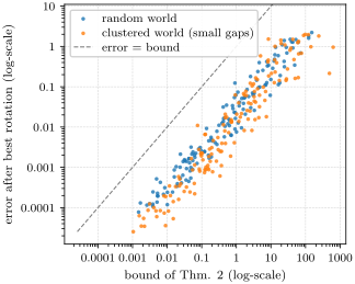
For whitened MSE, Theorem 2 bounds the best rotational mismatch by the difference between the two normalized positive-pair kernels, divided by a spectral gap. The modalities must share the same world-state marginal. Thus approximately shared positives give approximately shared representations when the relevant eigenspace is stable; a small gap weakens the guarantee.
Theorem 2: Kernel Mismatch Bounds Misalignment
Let share the marginal , let be their spectral embeddings (any orthonormal top- eigenvectors if has ties), and let be the eigengap of . Then
Equation
(Proof in Appendix A, empirical validation in Figure 2.)
What pairs are for.
Whitened unpaired clouds have identical first and second moments, so those moments cannot identify their relative rotation. Enough paired states spanning the embedding space determine it by orthogonal Procrustes [55]. Higher-order geometry can also identify a map without pairs, but this needs additional structure.
The experiments often map unequal-dimensional spaces with a row-orthonormal matrix. Such rectangular maps are useful operationally but are not the equal-dimensional rotations covered by the exact theorem.
Proposition 2: Pairs Identify the Rotation
In the setting of Sections 2.1 and 2.1, (i) every rotation of a whitened embedding is whitened, so no statistic of the first two moments of unpaired samples from two modalities identifies the rotation between them; (ii) if the embeddings of world states span , the rotation with is the unique minimizer over of (orthogonal Procrustes). (Proof in Appendix A.)
2.3 Good-View and Bad-View JEPAs
Let an observation contain a shared world state and independent modality-specific nuisance. Theorem 3 lower-bounds rotational mismatch using how much embedding variation is explained by the world state. Retaining nuisance therefore obstructs exact alignment.
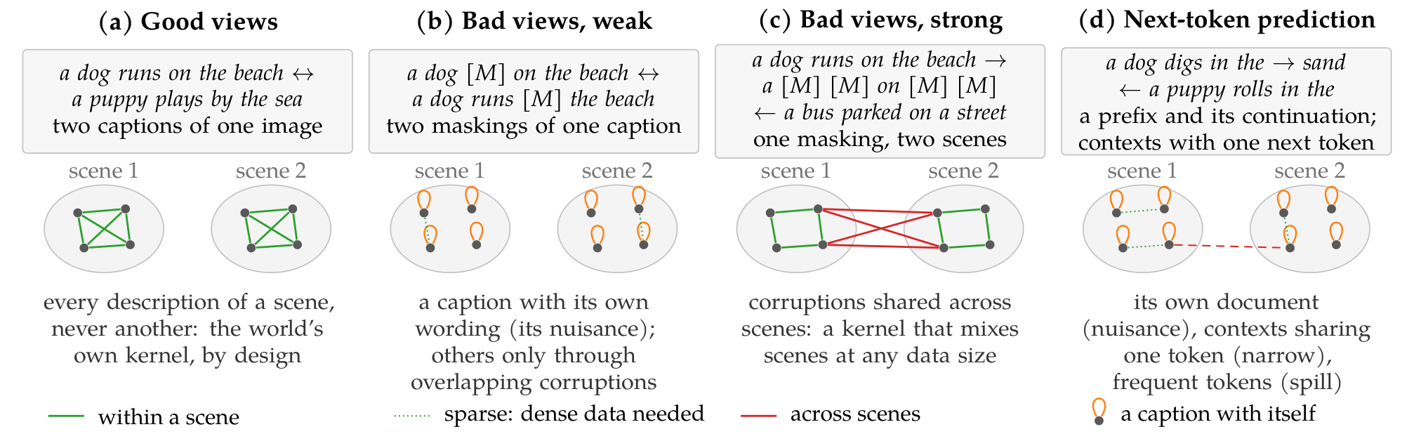
Good views independently resample nuisance while preserving the state. Under the stated spectral condition, their leading eigenfunctions ignore nuisance. For the analyzed bad-view product kernel, persistent nuisance enters the representation when its eigenvalues outrank state directions; each selected nuisance direction contributes to an irreducible mismatch. Bad views do not necessarily fail: the relative correlations determine the outcome.
Theorem 3: Nuisance Costs Alignment
Let and be centered, whitened encoders of two modalities into . Over paired observations of one world state with independent nuisances,
Equation
and if and only if is a function of the world state alone. (Proof in Appendix A.)
Proposition 3: Good Views Ignore Nuisance, Bad Views Capture It
Take the objective of Section 2.1. (i) If , a good-view JEPA learns a function of the world state alone (): good-view JEPAs of any number of modalities with the same world kernel agree up to one rotation each on every observation, although every state has many. (ii) Let a bad-view JEPA corrupt state and nuisance independently, let be the correlation that two corruptions of one observation keep along the -th direction of the state, and the largest they keep along a direction of the nuisance. If its kernel has a gap after its -th eigenvalue, it spends of its directions on nuisance, so that its alignment error with any centered, whitened encoder of another modality is at least , and if and only if . (Formal statement and proof in Appendix A.)
Views and data together.
Theorem 4 extends the analysis to general observations by separating state and nuisance components of the positive-pair operator. Agreement is controlled by differences between the induced world kernels, state–nuisance mixing, and spectral separation from nuisance directions. The bound is informative only when the required gaps dominate these perturbations.
Theorem 4: Views and Data Set the World Kernel
Take the objective of Section 2.1 on the observations of each modality , and let the -th eigenvalue of exceed both the next one and the share of nuisance its positives keep. (i) Every spectral solution is within of a rotation of the spectral embedding of , where grows with how much positive pairs mix world state with nuisance and vanishes when they do not. (ii) Over paired observations of two modalities,
Equation
with the misalignment of the spectral embeddings of and , which Section 2.2 bounds. (Formal statement and proof in Appendix A.)
How much data, and which.
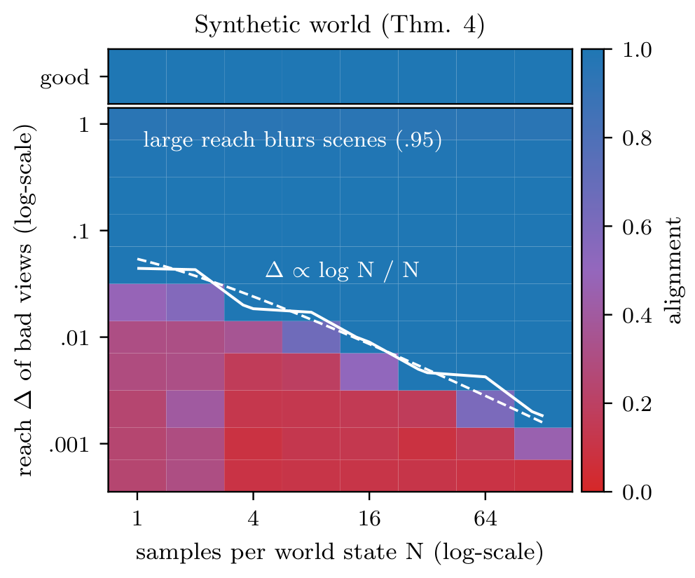
Views and dataset coverage jointly determine which observations become connected. Weak augmentations may need dense data to link observations of one state; augmentations that connect different states can impose a ceiling even with more data. Synthetic experiments illustrate both effects, including a reduced bad-view ceiling when qualitatively different data are mixed.
2.4 Next-Token Prediction is a Bad-View JEPA
Next-token cross-entropy can be written exactly as a generalized two-encoder JEPA objective: a context–target similarity term plus a log-sum-exp regularizer. At population optimum with sufficient rank and full support, logits recover conditional token probabilities up to a context-dependent offset.
This factorization is identifiable up to an invertible change of coordinates, not merely a rotation. The argument that a prefix and continuation retain shared linguistic nuisance is a proposed explanation of the experiments. It is not a corollary of the one-space, whitened spectral theorem, nor a result about all predictive world models.
Proposition 4: Next-Token Prediction Has the Form of a JEPA
Let a context be embedded by and tokens by a table . The next-token loss with a linear softmax head is
Equation
(i) This has the structure of a JEPA, generalizing (1) to two encoders and an anti-collapse term that depends on the target encoder: context encoder , target encoder , inner-product prediction, positives drawn from within one sequence. (ii) does not depend on the target token , and as , so the temperature-scaled loss approaches the margin , which vanishes iff the target attains the maximal logit. (iii) With full-support conditionals and large enough, minimizers satisfy , a set invariant under (, ), so is identified at best up to an invertible linear map, not a rotation. (Proof in Appendix A.)
3 Good Views Improve Alignment
The controlled experiments train image and text encoders separately, varying whether positive views come from one observation or several observations of the same scene.
Setup.
Flickr training uses 29,000 images with five captions each. Image encoders receive crops; text JEPAs receive either masked spans of one caption or different captions describing one image. A 33M-parameter BERT-S backbone also trains with causal next-token prediction, including a control that sees two captions per image.
JEPA models share LeJEPA/SIGReg training components [5]. Default runs use 200 epochs and three seeds. Epoch and image exposure are matched, but JEPA and next-token training process different numbers of text tokens per step.
Metrics.
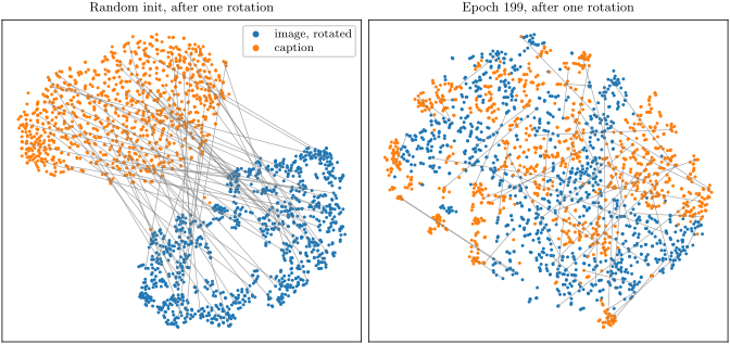
Mutual 10-NN measures agreement between neighborhood structures without fitting a cross-modal map. Retrieval instead fits an orthogonal map on 1,014 validation pairs and evaluates 1,000 held-out pairs. Chance is 0.01 for the neighborhood score and 0.001 for R@1.
| Text encoder | mutual 10-NN | R@1 | R@5 |
|---|---|---|---|
| Good-view JEPA | .062.003 | .044.002 | .133.004 |
| Bad-view JEPA | .047.001 | .027.002 | .095.003 |
| Next-token | .042.001 | .021.002 | .077.005 |
| Next-token, pairs | .043.001 | .023.003 | .083.008 |
| Random init | .010 | .001 | .011 |
| Chance | .010 | .001 | .005 |
3.1 Good Views Align Across Modalities
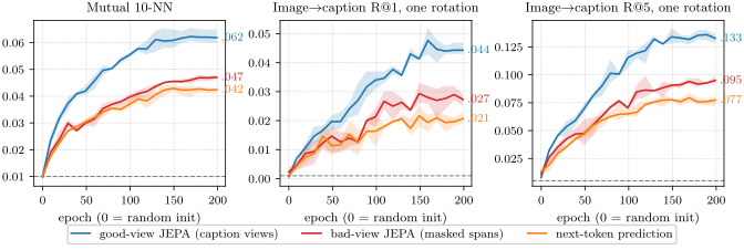
Good-view training reaches mutual 10-NN 0.062 and R@1 0.044, compared with 0.047/0.027 for bad-view training and 0.042/0.021 for next-token prediction. Giving next-token prediction a second caption scarcely changes these results.
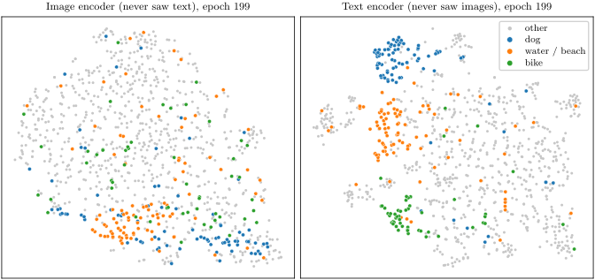
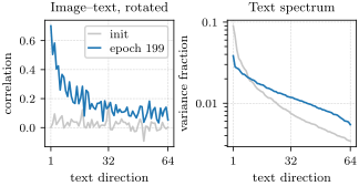
Agreement concentrates in leading principal directions. Estimated state-explained variation is higher for good views, and measured rotation errors exceed the nuisance-based lower bounds. These finite-sample diagnostics are consistent with the proposed mechanism; they do not verify all population assumptions.
3.2 Trimming Makes Good Views, the Rest Barely Matters
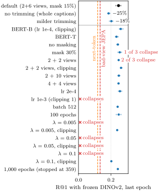
With a frozen DINOv2 image encoder, trimming captions is the largest tested recipe effect: removing it reduces R@1 from 0.246 to 0.185. Other individual changes have smaller mean effects in the reported sweep.
Training stability still matters. Some runs collapse, including three of 36 default runs without gradient clipping. Clipping helps but does not eliminate collapse under every learning-rate and regularization setting. Hyperparameters were tuned for good-view JEPA rather than equally optimized for all objectives.
3.3 Good Views Help on Both Sides
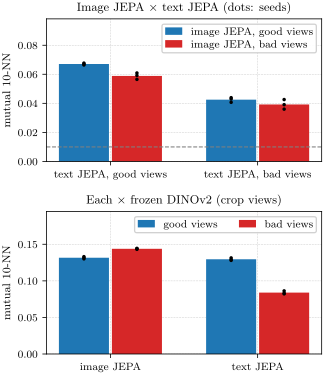
On MSR-VTT, good image views use different frames and good text views use different captions of one clip. Mutual 10-NN rises from 0.039 with both sides bad to 0.067 with both good; improving only text gives 0.059 and only images 0.043.
Agreement with an independently pretrained image encoder can favor a different recipe: crop-trained images align better with DINOv2 than frame-trained images. Positive-view compatibility matters in addition to within-dataset retrieval.
3.4 Good-View JEPAs Beat a Pretrained Language Model and Approach Pair-Trained Encoders
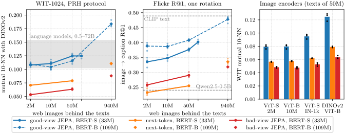
Against frozen DINOv2, good-view Flickr text training reaches R@1 0.246, versus 0.133 for bad views, 0.118 for next-token prediction, and 0.135 for pretrained Qwen2.5-0.5B. These compare in-domain training with an out-of-domain pretrained model.
CLIP and supervised MPNet remain stronger on this retrieval setting at 0.320 and 0.300, although their mutual-neighborhood scores are lower. More fitting pairs, training text, or model capacity can improve retrieval; neither metric alone establishes a universal encoder ranking.
| Text encoder, vs. frozen | mutual | R@1, rotation fit on | |
|---|---|---|---|
| DINOv2 ViT-B/14 | 10-NN | 1k pairs | 30k pairs |
| Qwen2.5-0.5B | .098 | .135 | .240 |
| BERT-base | .093 | .149 | .273 |
| bad-view JEPA | .132.001 | .133.007 | .207.008 |
| next-token | .122.001 | .118.002 | .213.004 |
| early-stopped | .124.002 | .134.008 | – |
| next-token, pairs | .132.002 | .137.004 | .247.016 |
| good-view JEPA | .232.006 | .246.015 | .346.007 |
| good-view JEPA, BERT-B | .245 | .273 | .363 |
| good, BERT-T, +COCO | .228 | .238 | .335 |
| good, +COCO | .228 | .256 | .367 |
| good, BERT-B, +COCO | .233 | .285 | .400 |
| good, BERT-L, +COCO | .227 | .269 | .376 |
| good-view JEPAs on Recap texts, no Flickr or COCO caption | |||
| texts of 2.16M images | .204.004 | .236.019 | .335.016 |
| BERT-B | .214.003 | .272.010 | .388.014 |
| texts of 10M images | .205.004 | .243.004 | .348.010 |
| BERT-B | .219.003 | .280.003 | .387.007 |
| texts of 50M images | .219.002 | .283.002 | .376.006 |
| BERT-B | .236.002 | .300.011 | .408.003 |
| texts of 100M images | .229.001 | .309.007 | .402.007 |
| texts of 940M, BERT-B | .257 | .349 | .464 |
| all-mpnet-base-v2 | .189 | .300 | .481 |
| CLIP B/32 text | .167 | .320 | .489 |
4 Next-Token Prediction Scales Poorly Compared to Good-View JEPAs
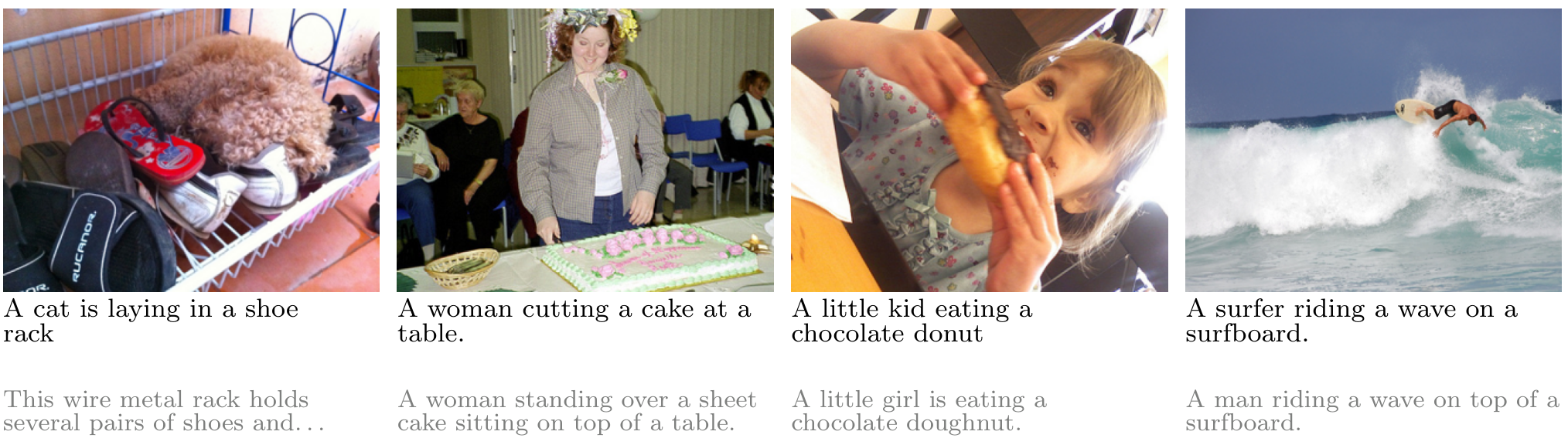
Scaling experiments train text encoders on grouped alt-text and synthetic captions associated with web images. The JEPA never receives pixels, but the grouping and recaptioning carry visual supervision.
4.1 Good Views Scale on Web Text
Recap-DataComp supplies an alt-text and two LLaVA captions per image [34]. A 33M good-view JEPA improves WIT alignment from 0.034 after Flickr training to 0.108 using texts from 2.16M images and about 0.125 at 50–100M images.
Matched-data comparisons favor good views: at 2.16M images, good-view, bad-view, and next-token scores are 0.108, 0.053, and 0.071. Better captions also help independently of the view objective; model width does not improve every alignment metric consistently.
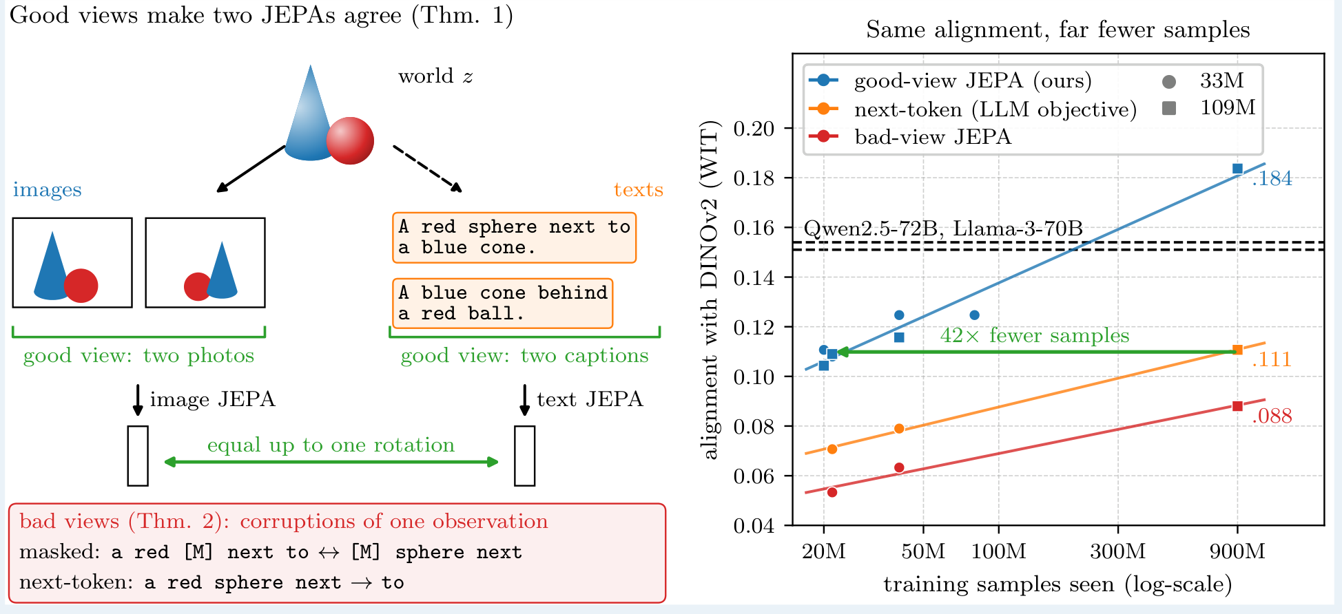
4.2 Good Views Need 42 Times Fewer Samples
The reported 42× comparison matches approximately 0.11 WIT alignment using 21.6M training items for good-view JEPA versus 900M for next-token prediction. These counts include repeated exposure; they are not unique images or tokens. Because JEPA reads three texts per item, the corresponding token ratio is about 14×, while the unique-image ratio is about 435×.
The runs use different learning rates and batch sizes, and no earlier checkpoint of the 900M-item next-token run was evaluated. This is an observed comparison between two training recipes, not a measured minimum sample requirement.
4.3 A 109M Text JEPA Beats Language Models up to 72B Parameters
A 109M good-view JEPA trained for 900M items from the 940M-image text corpus reaches mean WIT alignment 0.184 across three reported seeds, versus 0.111 for matched-scale next-token prediction, 0.088 for bad-view JEPA, and 0.154 for Qwen2.5-72B. Other tested image encoders and alignment metrics support the good-view advantage.
The three-seed mean excludes a fourth run whose effective SIGReg weight was doubled and whose WIT score was 0.121; the four-run mean is 0.168. The regularization choice followed inspection of WIT results. LLaVA recaptioning inherits CLIP-based vision supervision, so these are not encoders trained without any image–text-derived information.
| WIT, DINOv2-B | WIT | COCO | Flickr | ||
| Text encoder | 10-NN | CKA | CLIP-H | 10-NN | R@1 |
| good-view JEPA | .184 | .507 | .230 | .161 | .478 |
| next-token | .111 | – | .146 | – | .335 |
| bad-view JEPA | .088 | – | .116 | – | .318 |
| Qwen2.5-72B | .154 | .418 | .210 | .108 | – |
| Llama-3-70B | .151 | .380 | .206 | .113 | – |
| CLIP B/32 text | .124 | .339 | .159 | .132 | .489 |
| all-mpnet-base-v2 | .118 | .390 | .159 | .156 | .481 |
4.4 A Scaling Law for the PRH
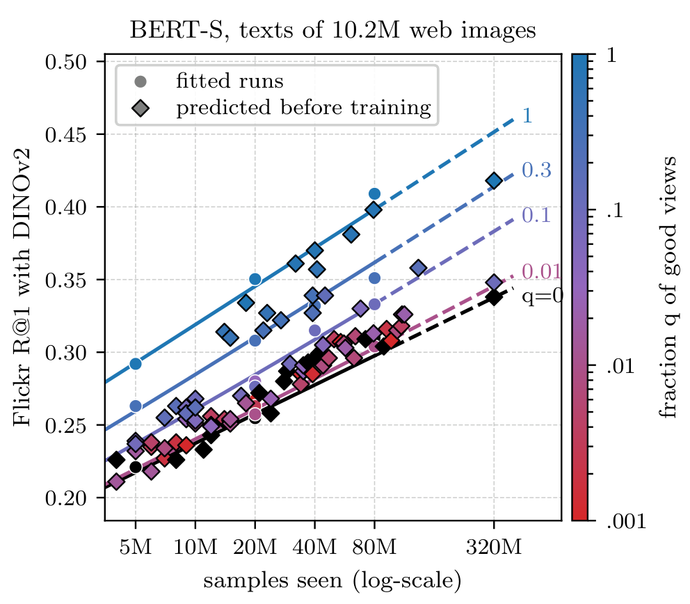
An empirical law relates retrieval to training items, unique images, and the fraction of good views. Fitted on 45 configurations, it predicts 85 subsequent runs with RMSE 0.0093, close to the 0.0096 variation between seed reruns.
Its exponents are weakly identified, and extrapolation to 320M items with repeated data overpredicts good-view retrieval. The formula omits a repeated-data penalty and applies to one studied recipe; it is not derived from the representation theorem.
Equation 7
| (7) |
5 Platonic Representations as a Tool
Shared geometry supports two distinct applications: captioning with a map fitted on paired examples, and estimating the map from unpaired embedding clouds.
5.1 Captioning Without Training a Network on Image–Caption Pairs
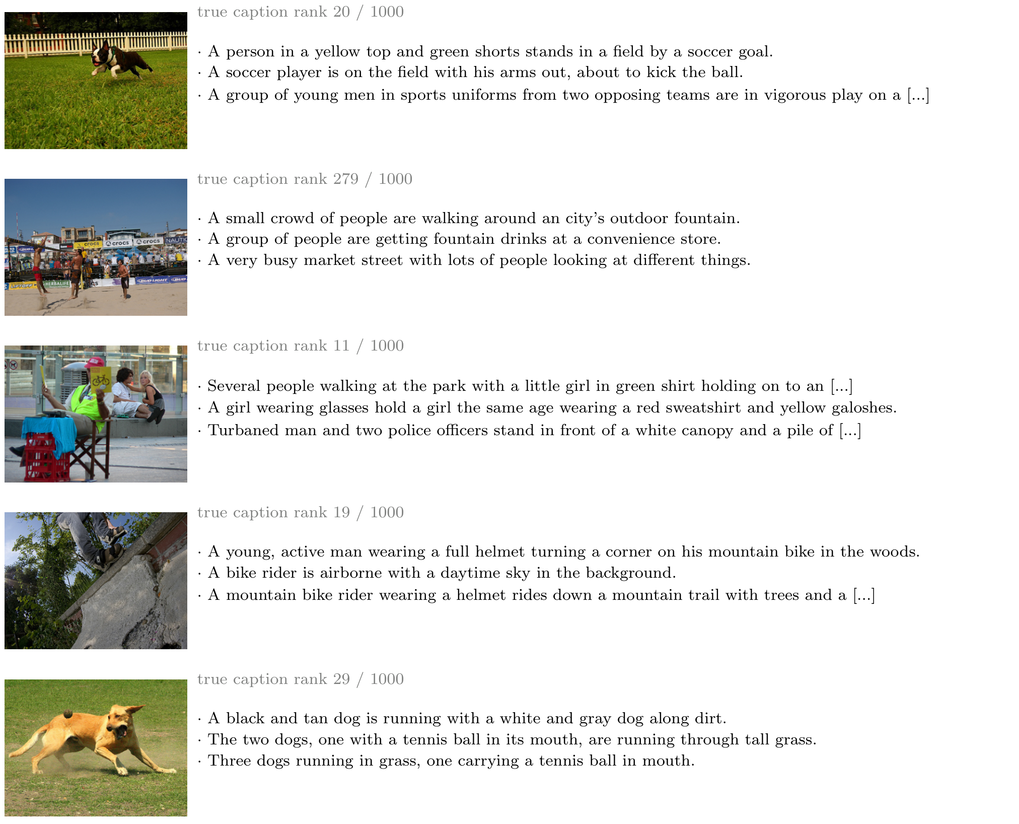
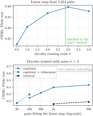
A text-only decoder reconstructs captions from noisy, frozen JEPA embeddings. At inference, a frozen image encoder and fitted orthogonal map supply its input. Noise compensates for residual image–text mismatch, following an approach related to noise-injected caption decoding [43].
The base captioner obtains Flickr CIDEr 0.396 using 1,014 map-fitting pairs and 0.431 using 30,000. With Flickr pairs only for the map and Flickr plus COCO captions for decoder training, it transfers to COCO at 0.668. CIDEr uses a 0–1 scale throughout this paper.
The strongest configuration combines a pretrained language decoder, a web-trained text JEPA, frozen image encoders, and consensus decoding. It reaches COCO CIDEr 0.838 with its map still fitted on 30,000 Flickr pairs. A rectangular row-orthonormal map performs better on COCO transfer than unconstrained linear or nonlinear maps in the tested comparison. This supports a useful constraint, without proving the exact equal-dimensional theorem applies.
Averaging eight frame embeddings also transfers the photo-trained captioner to video: MSR-VTT CIDEr is 0.246 without video training. It remains below the cited specialized video systems and often misses actions or speech.
5.2 Alignment Without Any Pair
A separate experiment uses the clustering and optimal-transport method of Schnaus et al. to align unpaired clouds [54]. Images and captions come from disjoint COCO training halves; evaluation pairs and class labels are not used to fit the map.
Across three JEPA training seeds and five alignment seeds each, the 109M model reaches FOSCTTM 0.018 and ImageNet-100 top-5 accuracy 64.4%, versus 0.018 and 47.6% for the Qwen3-8B rerun. CLIP still leads on FOSCTTM and ImageNet-100 at 0.006 and 68.7%. Bad-view JEPA also aligns well on COCO, so this setting does not isolate good views as the sole explanation.
On the smaller Flickr pools, only web-trained good-view JEPAs clearly exceed chance in the tested set. Pair-free captioning reaches CIDEr 0.158±0.042, or 0.208 for the map selected by the unpaired training objective, versus 0.430 with a 30,000-pair map. Fully pair-free results should therefore be distinguished from the strongest paired-map captioner.
| Text encoder (runs) | FOSCTTM | C-10 | C-100 | IN-100 |
| good-view JEPA, 109M (15) | .018 | 86.0 | 67.2 | 64.4 |
| good-view JEPA, 33M (15) | .036 | 83.2 | 60.9 | 57.9 |
| bad-view JEPA, 109M (5) | .026 | 78.1 | 55.3 | 46.7 |
| next-token, 109M (15) | .287 | 25.5 | 19.9 | 20.3 |
| Qwen3-8B, rerun (5) | .018 | 83.4 | 61.7 | 47.6 |
| MPNet, rerun (5) | .043 | 70.2 | 45.6 | 45.4 |
| their best, these data | .02 | 80 | 58 | 46 |
| their best, any setting | .01 | 82 | 62 | 56 |
| CLIP B/32 text (5) | .006 | 84.0 | 67.0 | 68.7 |
| 82,783 pairs | .002–.005 | 83–92 | 65–85 | 57–88 |
6 Related Work
The theory connects spectral accounts of self-supervised learning [4] [19] with prior work on augmentation, identifiability, and shared representations [74] [22]. Earlier cross-space matching methods already use geometry to align independently trained encoders [1] [54].
The experimental contribution is to connect positive-view design to alignment across model scales and to demonstrate useful downstream maps. Prior captioning systems often use jointly trained image–text encoders; this approach separately trains its encoders but still uses visual caption generation and, for its strongest captioner, paired map fitting.
7 Conclusion
Shared positive relationships provide sufficient conditions for common geometry, and different observations of one scene improve alignment in the tested JEPA recipes. They do not establish inevitable convergence for arbitrary models.
No experiment exactly satisfies Theorem 1: observations can be lossy, practical encoders and optimization are restricted, SIGReg differs from exact whitening, and image training often uses views classified as bad by the theory. Synthetic captions inherit multimodal supervision; good-view grouping uses scene correspondences. Hyperparameters were tuned for good-view JEPA, with WIT used to select the largest model's regularization. Evidence remains strongest for the controlled view comparisons and the reported image–text protocols.
Acknowledgments
The acknowledgments credit discussions, infrastructure, and research support. The authors provide code, experiment details, and additional results with the paper.
Appendix A Proofs
The appendix retains the formal objectives, statements, and derivations. The proofs establish sufficient conditions in the specified population models; numerical checks test the algebra rather than real-world applicability.
A.1 Notation and Objectives
Notation.
The notation represents a finite world by its probability diagonal matrix, symmetric positive-pair matrix, and normalized kernel. Embeddings use the probability-weighted inner product; centering removes the constant eigenfunction. Orthogonal alignment is evaluated in this weighted space.
Objectives of the form ( 1 ).
Whitened MSE reduces to maximizing a kernel trace under centered orthonormal coordinates. Rotation-invariant regularizers also include covariance-based objectives and the expected SIGReg penalty. Invariance alone does not establish uniqueness of minimizers; that remains a separate hypothesis outside the whitened spectral case.
A.2 The Platonic Representation Theorem ( Section 2.1 )
Injective renderings give a bijection between modality encoders and world-state embeddings, making their shared-positive objectives identical. Rotation uniqueness then proves Theorem 1. For whitened MSE, the Ky Fan variational principle selects the leading nonconstant eigenspace; the spectral gap makes that subspace unique.
Lemma 1: Renderings Only Change Coordinates
If is injective, is a bijection between encoders on and functions , and .
Equation
A.3 When Positives Differ ( Section 2.2 )
A Davis–Kahan perturbation argument bounds changes in the selected eigenspace when positive-pair kernels differ [71]. Orthogonal Procrustes converts the subspace comparison into the stated embedding error. The appendix also explains why whitening erases the first-two-moment information needed to choose a rotation, whereas full-rank paired observations identify it.
Equation
A.4 Good-View and Bad-View JEPAs ( Section 2.3 )
Conditioning on the world state separates shared variation from nuisance. Covariance and nuclear-norm inequalities yield the nuisance lower bound. Product-kernel eigenfunctions explain when persistent nuisance outranks state information; a block-operator perturbation argument then handles state–nuisance mixing in the general case.
Proposition 3 (Formal): Good Views Ignore Nuisance, Bad Views Capture It
Modality has a finite nuisance set with distribution , , the state and the two nuisances being mutually independent, and renders injectively as ; a paired image and caption are with independent. A good-view JEPA’s positives are with and independent; a bad-view JEPA’s are two corruptions of one observation , which share its nuisance. Take the objective of Section 2.1. (i) A good-view JEPA’s kernel is ; if , its minimizers are , functions of the state alone, and good-view JEPAs of any number of modalities with the same world kernel agree up to one rotation each on every observation: Section 2.1 when every state has many observations. (ii) Let a bad-view JEPA corrupt state and nuisance independently, with and row-stochastic with stationary laws and , so that corrupted views are observations with the law of clean ones, and let and be the eigenvalues of the Markov operators on and on of two corruptions of one state and of one nuisance ( the adjoint; for ), with eigenfunctions and (). Its kernel then has eigenvalues with eigenfunctions ; let be those with , with multiplicity. If , of the top have , its minimizers have with zero eigenvalues, i.e., , and by Section 2.3 their alignment error with any centered, whitened encoder of the other modality is at least . Moreover if and only if .
Theorem 4 (Formal): Views and Data Set the World Kernel
Let modality have finitely many observations , each of a world state , with law () of state marginal , and let be any symmetric law on pairs of observations whose marginal is , the law on which encoders are whitened and evaluated: good views, ; corruptions of one observation that leave the law of observations invariant (, as in Section 2.3); or a mix. Its induced world kernel is the probability that a positive pair joins an observation of to one of . Let be the conditional expectation onto functions of the state in , let be the largest eigenvalue of the compression to nuisance functions (), which measures how much of its own nuisance a positive keeps ( if every state has one observation), and let and be the operator and Hilbert–Schmidt norms of , which measure how much state and nuisance mix. Take the objective of Section 2.1 with , let be the eigenvalues of on (), and suppose . (i) Every spectral solution of (orthonormal top- eigenfunctions of on ) is close to a spectral embedding of its induced world kernel,
Equation
and . (ii) For two modalities of one world, over paired observations from any coupling with and ,
Equation
where is at most by Section 2.2, with the gap of .
Special cases and scope.
Independent nuisance resampling eliminates the nuisance block and mixing term. Bad-view product kernels have no mixing but can retain nuisance eigenvalues large enough to displace state directions. Merging observations of one state can reduce nuisance; connecting different states changes the world kernel. Soft architectural biases and noninjective renderings require analysis beyond the exact theorem.
A.5 Next-Token Prediction is a Bad-View JEPA ( Section 2.4 )
Expanding cross-entropy produces the context–target attraction term and log-sum-exp regularizer. At low temperature the normalized objective approaches a margin form. Full-support optimum logits encode log conditional probabilities, while their two-factor decomposition admits general invertible coordinate changes. These calculations do not import the whitened JEPA nuisance theorem into next-token prediction.
A.6 Numerical Checks
Random finite-world checks verify the stated perturbation and nuisance inequalities, including 300 differing-kernel pairs. Observed errors remain below the analytical bounds. These checks support implementation of the formulas; they do not test their assumptions for trained neural encoders.
Appendix B Experimental details
Code.
Experiments use stable-pretraining's LeJEPA/SIGReg implementation. A multilayer projector and 1,024 random SIGReg projections regularize the latent distribution. The supplied implementation and retained settings specify the reproduction recipe.
Image encoder.
The small image encoder is ViT-S/16 with CLS pooling. Two global and six local crops undergo color and blur augmentations. Frozen pretrained vision encoders are evaluated separately from image JEPAs trained from scratch.
Text encoders.
The main small text backbone has 12 layers, six attention heads, width 384, and a 64-token limit. JEPA uses CLS pooling; causal next-token models use mean pooling for evaluation, which performs better than their last-token representation. Good views sample different captions of one image before trimming and masking.
Optimization.
Default training uses AdamW, batch 256, learning rate 5×10⁻⁴, weight decay 0.05, and 200 epochs with warmup and cosine decay. Longer and larger runs use revised rates and gradient clipping. Distributed training changes the effective SIGReg weight unless its scaling is accounted for; the largest-model appendix reports the resulting seed discrepancy.
MSR-VTT.
MSR-VTT uses 7,010 training clips, 1,990 map-fitting clips, and 1,000 retrieval-test clips. Good views sample different frames or captions from one clip; bad views reuse one observation. Runs train for approximately 21,600 updates and average three seeds.
PRH protocol.
The PRH evaluation uses 1,024 WIT image–caption pairs, the first caption per image, and layerwise visual CLS and mean-pooled language features. Features are clipped and normalized before mutual 10-NN evaluation. Reported scores maximize over layer pairs, making protocol and dataset size important when comparing small differences.
Appendix C Additional results
The additional experiments probe training stability, data quality, uncertainty, benchmark overlap, captioning, and alternative encoders. All original result tables and qualitative examples are retained.
| captioncaption R@1 | mutual 10-NN (projector) | R@1 (projector) | whitened R@1 (projector) | |
|---|---|---|---|---|
| Good-view JEPA | .606 | .064 | .030 | .034 |
| Bad-view JEPA | .381 | .044 | .018 | .022 |
| Next-token prediction | .331 | – | – | – |
| TF-IDF | .442 | – | – | – |
| Random init | .178 | – | – | – |
Text encoders alone.
Table 5 evaluates text encoders and projector outputs without jointly retraining the image encoder. Retrieval and neighborhood agreement can rank models differently. Later figures preserve captioning examples, including errors and differences between fitted maps.
Next-token overfitting.
The Flickr next-token model overfits: validation loss rises after epoch 29. Selecting that validation-loss minimum improves R@1 from 0.118 to 0.134, still below good-view JEPA's 0.246. A test-selected checkpoint is reported diagnostically, not used as the main result. JEPA also processes more caption tokens per step.
Nuisance on real encoders.
Real-encoder nuisance estimates whiten principal components and use repeated captions to estimate scene-explained covariance. A finite-caption correction and eigenvalue clipping stabilize the estimate. Higher estimated state information accompanies lower alignment error, but these are finite-sample proxies for the population quantities.
| Text encoder (Flickr) | scene-explained | bound | error | scene-explained | bound | error |
|---|---|---|---|---|---|---|
| Good-view JEPA | .804.003 | 12.6 | 33.5 | .654.005 | 88.6 | 157.0 |
| Bad-view JEPA | .655.005 | 22.1 | 39.4 | .507.003 | 126.1 | 171.5 |
| Next-token | .608.001 | 25.1 | 40.3 | .440.002 | 143.4 | 176.6 |
| trained on Recap texts only (seed 0), measured on the same Flickr captions | ||||||
| Good-view JEPA, 50M images | .802 | 12.7 | 32.4 | .642 | 91.7 | 156.8 |
| Bad-view JEPA, 50M images | .673 | 20.9 | 37.6 | .506 | 126.4 | 168.7 |
| Next-token, 50M images | .618 | 24.4 | 40.1 | .483 | 132.3 | 171.0 |
| Good-view JEPA, 100M images | .806 | 12.4 | 32.0 | .661 | 86.9 | 153.7 |
| Good-view JEPA, BERT-B, 940M images | .830 | 10.9 | 30.0 | .722 | 71.1 | 145.3 |
Which texts give the gain.
Caption quality and view construction both contribute. Alt-text plus text-only Qwen paraphrases gives WIT alignment 0.060, compared with 0.107 when visual recaptions are available. Even bad-view training benefits from recaptions. The largest gains therefore cannot be attributed to a text-only objective independently of the captioner's visual knowledge.
| Texts of | texts per image | views | WIT (DINOv2-B) | Flickr R@1 | scene-explained |
|---|---|---|---|---|---|
| 2.24M images | alt-text, two LLaVA recaptions | good | .107 (.095–.115) | .339 (.336–.344) | .793 |
| 2.24M images | alt-text, text-only paraphrase | good | .060 (.058–.061) | .233 (.230–.235) | .654 |
| 2.24M images | two LLaVA recaptions | good | .080 (.076–.082) | .348 (.346–.351) | .778 |
| 2.24M images | alt-text | bad | .055 (.054–.056) | .180 (.179–.180) | .606 |
| 50M images | alt-text, two LLaVA recaptions | good | .125 (.118–.129) | .376 (.370–.381) | .802 |
| 50M images | two LLaVA recaptions | good | .096 (.093–.100) | .386 (.373–.396) | .789 |
| 50M images | alt-text, two LLaVA recaptions | bad | .063 (.062–.066) | .290 (.283–.301) | .673 |
| 50M images | two LLaVA recaptions | bad | .092 (.090–.093) | .325 (.323–.329) | .734 |
| 50M images | alt-text | bad | .056 (.056–.057) | .199 (.193–.203) | .618 |
Data kind in the synthetic world.
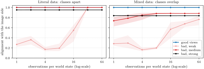
Synthetic worlds separate denser sampling from adding different kinds of observations. More samples can connect nearby views, but mixing data types leaves a bad-view alignment ceiling in the studied construction. Good views recover the intended state geometry under the model's exact assumptions.
The scaling law in detail.
The scaling fit evolved from smaller configuration sets to 45 cells; the final held-out exercise covers 85 prospective runs. Several exponent combinations fit similarly, so individual exponents should not be interpreted as established laws. At 320M items, predictions overshoot good-view retrieval after many passes through the same images, exposing the missing repeated-data effect.
Equation
Robustness of the good-view recipe.
Good-view alignment can collapse after a strong earlier checkpoint. Clipping reduces failures, but high learning rates and some regularization weights still collapse; some failed larger runs are excluded. Very weak regularization can produce a low-rank representation despite reasonable retrieval. Best-checkpoint columns selected using test retrieval are diagnostics rather than the main selection rule.
| Good-view text JEPA, one change from the default | last-epoch R@1, seeds 0 / 1 / 2 | mean | best∗ (epoch), seed 0 |
|---|---|---|---|
| Default: 2 + 6 views, mask 15%, lr , | .248 / .260 / .230 | .246 | .276 (99) |
| BERT-B (768 wide; lr , clipping 1) | .273 / .252 / .255 | .260 | .275 (189) |
| BERT-T (192 wide) | .244 / .229 / .228 | .234 | .254 (149) |
| no masking | .236 / .246 / .244 | .242 | .259 (109) |
| mask 30% | .243 / × / .264 | .254 | .266 (129) |
| no trimming (whole captions) | .193 / .182 / .180 | .185 | .242 (79) |
| milder trimming (70–100% / 40–80%) | .211 / .204 / .191 | .202 | .268 (59) |
| 2 + 2 views | .247 / × / × | .247 | .257 (129) |
| 2 + 2 views, clipping 1 | .260 / .258 / .267 | .262 | .272 (159) |
| 2 + 10 views | .254 / .247 / .243 | .248 | .262 (119) |
| 4 + 4 views | .242 / .249 / .248 | .246 | .258 (109) |
| lr | .265 / .246 / .253 | .255 | .270 (169) |
| lr (clipping 1) | collapses | – | – |
| batch 512 | .239 / .243 / .240 | .241 | .245 (129) |
| 100 epochs | .233 / .261 / .248 | .247 | .239 (59) |
| collapses | – | .196 (29) | |
| , clipping 1 | .238 | .238 | .242 (119) |
| collapses | – | .242 (89) | |
| , clipping 1 | collapses | – | .162 (19) |
| collapses | – | .191 (79) | |
| , clipping 1 | .202 | .202 | .215 (149) |
| 1,000 epochs, stopped at 359 (lr , clipping 1) | .242 (359) | .242 | .278 (99) |
| Captioner (Flickr test) | BLEU-4 | CIDEr |
|---|---|---|
| Oracle: decode the true caption embedding | .261 | .628 |
| Image rotation (30k pairs) decode | .185 | .431 |
| Image rotation (1,014 pairs) decode | .173 | .396 |
| Image rotation (300 pairs) decode | .146 | .317 |
| Image rotation (100 pairs) decode | .119 | .244 |
| + unpaired refinement (100 pairs) | .138 | .294 |
| + unpaired refinement (30 pairs) | .099 | .169 |
| Retrieve nearest caption (30k pairs) | .065 | .188 |
| Retrieve nearest caption (1,014 pairs) | .054 | .158 |
| Random rotation | .059 | .043 |
| Captioner (CIDEr; one rotation from the 30k Flickr pairs) | Flickr | COCO |
| Small decoder, DINOv2 ViT-B, in-domain text JEPA (Table 9) | .431 | .668 |
| Qwen2.5-1.5B decoder, web text JEPA, DINOv2 ViT-g (CLS) | .466 | .720 |
| + mean patch token | .480 | .756 |
| + captions as written (case, punctuation) | .479 | .765 |
| + DINOv3 ViT-L, concatenated | .496 | .806 |
| + consensus of 32 samples | .519 | .838 |
| Variants of the DINOv3 ViT-L row | ||
| DINOv3 ViT-7B instead of ViT-L | .507 | .816 |
| decoder first trained on 4M web sentences | .504 | .802 |
| map trained on the same pairs instead: any linear map | .531 | .635 |
| map trained on the same pairs instead: two-layer MLP | .498 | .585 |
| + consensus of 32 samples (the demo) | .538 | .832 |
| map trained on the same pairs instead: any linear map | .561 | .652 |
| map trained on the same pairs instead: two-layer MLP | .511 | .597 |
| Qwen2.5-3B decoder (captions-as-written row) | .460 | .730 |
Few pairs and no pairs.
Refinement on unpaired clouds helps when the initial paired map is underdetermined: with 100 pairs, Flickr CIDEr improves from 0.244 to 0.294. Thirty pairs reach 0.169. With no pairs, the original Flickr-only encoder and small clouds remain near chance; successful pair-free results use stronger web-trained representations and larger pools.
Video.
Averaging frames improves video alignment and captioning, but photo-derived descriptions frequently omit motion or speech. The main video result uses a map fitted on 30,000 Flickr pairs. A separate demo configuration adds 200,000 web pairs for map fitting and reaches CIDEr 0.268; it is not the same pairing budget.
| MSR-VTT test, 2,990 clips | CIDEr | BLEU-4 | METEOR | ROUGE-L |
|---|---|---|---|---|
| Ours: mean of 8 frames, rotation from 30k Flickr pairs, consensus of 32 | .246 | .166 | .206 | .444 |
| beam 3 | .222 | .154 | .204 | .432 |
| map from 30k Flickr and 200k web pairs (the demo’s) | .268 | .186 | .232 | .471 |
| middle frame instead of the mean of 8 | .242 | .172 | .219 | .457 |
| oracle: decode the text embedding of one human caption | .383 | .257 | .265 | .538 |
| CLIP ViT-B/32 encoders (400M image–text pairs), no MSR-VTT text; from Li et al. [33], Tab. 4 | ||||
| ZeroCap [60] | .058 | – | – | – |
| MAGIC [59] | .074 | – | – | – |
| DeCap, decoder on CC3M captions | .150 | – | – | – |
| DeCap, decoder on COCO captions | .186 | .147 | .204 | – |
| DeCap, decoder on MSR-VTT captions | .348 | – | – | – |
| MSR-VTT 1k-A (1,000 clips) | map fitted on | mutual 10-NN | textvideo R@1/5/10 | videotext R@1 |
|---|---|---|---|---|
| ours, mean of 8 frames | 30k Flickr pairs | .167 | 16.5 / 38.8 / 49.1 | 18.6 |
| ours, mean of 8 frames | 9k MSR-VTT clips | .167 | 19.3 / 45.6 / 57.9 | 20.5 |
| ours, middle frame | 30k Flickr, 200k web pairs | .148 | 14.5 / 33.1 / 44.9 | 17.1 |
| CLIP ViT-B/32 [35] | – (jointly trained) | – | 31.2 / 53.7 / 64.2 | 27.2 |
Alignment without any pair, in detail.
Pair-free alignment retains the published method's hyperparameters and five random seeds. Test pairs and labels score results only; method-seed selection uses the unpaired fitting objective. Some encoder and dataset combinations fail across most seeds, and Flickr retrieval varies substantially even for the strongest model.
The 109M results combine five alignment seeds within each of three training seeds. These 15 runs are nested rather than 15 independent trained encoders, which limits interpretation of the reported significance tests. CLIP remains stronger on some COCO metrics, and bad-view JEPA also succeeds there.
Decoder noise.
Decoder noise is chosen to approximate the cosine mismatch between aligned image and text embeddings. The initial calculation used test-set cosine; a later held-out validation calculation gives a similar recommendation near noise scale three. This supports the heuristic but does not make the original choice prospectively validation-only. Small score changes below about 0.01 are within the observed decoding variability.
Scaling the captioner.
The larger decoder fine-tunes Qwen2.5-1.5B on caption text, using a small network to convert the JEPA vector into ten soft-prompt tokens. Consensus decoding selects among sampled captions using agreement between candidates, without human reference captions at selection time [27].
Combining normalized DINOv2 and DINOv3 features improves the tested captioner. Text-only web pretraining improves some reconstruction measures without consistently improving benchmark transfer. The main strongest captioner still uses 30,000 paired examples for its cross-modal map.
Projector outputs.
Whitening projector outputs changes R@1 only slightly, from 0.030 to 0.034 in the reported comparison. Their existing near-isotropy limits the effect; this does not show whitening is irrelevant to other encoders or objectives.
Transfer to COCO.
A map fitted on 30,000 Flickr pairs transfers to COCO at R@1 0.113 among 5,000 candidates. Each modality can be centered using its own unpaired data. Fitting on half the COCO evaluation set and testing on the other half is a separate protocol with fewer candidates, so its score is not directly comparable.
Frozen image encoders.
Larger frozen image encoders can improve retrieval without producing the best captions. DINOv3-7B has strong retrieval, while DINOv2-g is more effective for some captioning settings. Concatenating DINOv2-g and DINOv3-L features yields a useful tested quality–cost compromise, not a general model ranking.
| BERT-B, texts of 50M images | BERT-S, 100M | |||||
| Frozen image encoder | features | mutual 10-NN | R@1 | R@5 | R@1 | R@5 |
| DINOv2 ViT-B/14 | CLS | .234 | .412 | .733 | .400 | .711 |
| DINOv2 ViT-L/14 | CLS | .242 | .437 | .745 | .410 | .732 |
| DINOv2 ViT-g/14 | CLS | .245 | .437 | .769 | .425 | .741 |
| DINOv2 ViT-g/14 | CLS + mean patch | .250 | .460 | .784 | .440 | .763 |
| DINOv3 ViT-L/16 | CLS | .209 | .436 | .722 | .414 | .703 |
| DINOv3 ViT-L/16 | CLS + mean patch | .234 | .514 | .792 | .489 | .780 |
| DINOv3 ViT-H+/16 | CLS | .181 | .353 | .625 | .342 | .607 |
| DINOv3 ViT-H+/16 | CLS + mean patch | .228 | .479 | .779 | .486 | .775 |
| DINOv3 ViT-7B/16 | CLS | .207 | .455 | .752 | .452 | .730 |
| DINOv3 ViT-7B/16 | CLS + mean patch | .231 | .531 | .803 | .523 | .798 |
| I-JEPA ViT-H/14 (IN-22k) | mean patch | .109 | .188 | .451 | .183 | .436 |
| I-JEPA ViT-g/16 (IN-22k) | mean patch | .140 | .246 | .502 | .234 | .491 |
| DINOv2-g + DINOv3-L | both, concatenated | .255 | .505 | .806 | .488 | .791 |
| DINOv2-g + DINOv3-7B | both, concatenated | .256 | .535 | .824 | .511 | .801 |
| Image JEPA | Text JEPA | mutual 10-NN | R@1 | R@5 |
|---|---|---|---|---|
| good views (frames) | good views (captions) | .067.001 | .032.006 | .099.009 |
| bad views (crops) | good views (captions) | .059.002 | .024.002 | .105.008 |
| good views (frames) | bad views (spans) | .043.002 | .020.005 | .063.002 |
| bad views (crops) | bad views (spans) | .039.003 | .017.002 | .072.009 |
| frozen DINOv2 ViT-B | good views (captions) | .129.002 | .085.006 | .258.011 |
| frozen DINOv2 ViT-B | bad views (spans) | .084.002 | .052.002 | .164.006 |
| frozen DINOv2 ViT-B | image JEPA, good views | .132.002 | .219.010 | .462.011 |
| frozen DINOv2 ViT-B | image JEPA, bad views | .144.001 | .285.005 | .559.008 |
Text-only quality.
Good-view training also improves semantic textual similarity: Flickr-trained good-view, bad-view, and next-token encoders score Spearman correlations 0.579, 0.528, and 0.430. More web text raises good-view performance to 0.632, below supervised MPNet's 0.834. Alignment gains therefore coexist with useful text semantics without implying state-of-the-art language understanding.
Uncertainty on WIT.
WIT contains only 1,024 pairs. Repeated 800-pair subsamples show that small gaps between the 50M-image JEPA and some pretrained language models have confidence intervals spanning zero. Larger matched-data good-view versus next-token gaps remain positive. Close cross-model rankings should be read with this uncertainty.
Image JEPAs trained from scratch.
Image JEPAs trained from scratch on web images or ImageNet generally preserve the ordering of good-view text above next-token and bad-view text. Their image augmentations are crops, classified as bad views in the theory. These experiments broaden empirical support without creating an exact test of its hypotheses.
Scaling to the texts of 940M images.
The largest study distinguishes a corpus associated with 940M unique images from the 900M items actually processed. Batch size, learning rate, and effective regularization differ from the smaller-scale runs.
Three good-view seeds score 0.191, 0.181, and 0.179 on WIT. A fourth seed with doubled effective SIGReg scores 0.121; including it lowers the mean from 0.184 to 0.168. The effective weight was chosen after inspecting WIT, so this benchmark contributed to model selection. Other vision-family comparisons are less decisive when all four runs are included.
| Text JEPA | texts of | global batch | samples seen | WIT (DINOv2-B) | Flickr R@1 |
|---|---|---|---|---|---|
| BERT-S | 100M images | 256 | 80M | .125† | .402† |
| BERT-B | 200M images | 256 | 89M | .125 | .447 |
| BERT-B | 200M images | 256 | 117M | .126 | .447 |
| BERT-B | 200M images | 256 | 160M | .126 | .451 |
| BERT-B | 940M images | 2,048 | 430M | .182 | .410 |
| BERT-B | 940M images | 2,048 | 580M | .182 | .463 |
| BERT-B | 940M images | 2,048 | 850M | .191 | .468 |
| BERT-B | 940M images | 2,048 | 900M | .191 | .464 |
| BERT-B, seed 1 | 940M images | 2,048 | 900M | .181 | .484 |
| BERT-B, seed 2 | 940M images | 2,048 | 900M | .179 | .485 |
| BERT-B‡ | 940M images | 2,048 | 900M | .121 | .477 |
| BERT-B, next-token, seed 0 | 940M images | 2,048 | 900M | .109 | .346 |
| BERT-B, next-token, seed 1 | 940M images | 2,048 | 900M | .111 | .332 |
| BERT-B, next-token, seed 2 | 940M images | 2,048 | 900M | .112 | .328 |
| BERT-B, bad views | 940M images | 2,048 | 900M | .088 | .318 |
WIT captions in the training texts.
The overlap search identifies at least 43 of 1,024 WIT captions in the training text. Removing them changes reported scores by at most 0.002. WIT image identities are unavailable, preventing a complete image-level audit.
Recovered image matches also include six Flickr test images and 50 of 5,000 COCO test images. Removing the latter changes alignment by at most 0.001. These checks bound the effect of identified overlap, not undiscovered duplicates or supervision inherited from the recaptioner.
WIT, PRH protocol.
Flickr-only encoders perform poorly on WIT across objectives, around 0.029–0.037. Training on web captions substantially improves this cross-domain measure. The retained table follows the PRH layer-pair maximum protocol, so it should not be equated with retrieval after fitting a single final-layer map.
| Qwen2.5 | Mistral | ours (33M), on the texts of Recap images | ours (109M) | |||||||
|---|---|---|---|---|---|---|---|---|---|---|
| 2.16M | 10M | 50M | 100M | 940M | ||||||
| Vision | 0.5B | 1.5B | 3B | 7B | 7B | good / bad / nt | good | good / bad / nt | good | good |
| DINOv2 ViT-S/14 | .092 | .101 | .110 | .110 | .126 | .099 / .052 / .065 | .102 | .114 / .062 / .074 | .114 | .166 |
| DINOv2 ViT-B/14 | .102 | .108 | .125 | .118 | .140 | .108 / .053 / .071 | .111 | .125 / .063 / .079 | .125 | .184 |
| DINOv2 ViT-L/14 | .114 | .123 | .139 | .137 | .157 | .111 / .057 / .075 | .115 | .130 / .068 / .085 | .131 | .196 |
| DINOv2 ViT-g/14 | .115 | .124 | .141 | .133 | .157 | .114 / .059 / .076 | .117 | .132 / .070 / .086 | .133 | .197 |
| ours, ViT-S, Recap 2M | .062 | .068 | .078 | .073 | .086 | .070 / .042 / .053 | .071 | .079 / .048 / .057 | .080 | .106 |
| ours, ViT-B, Recap 10M | .064 | .070 | .079 | .075 | .087 | .071 / .043 / .054 | .072 | .080 / .048 / .058 | .081 | .106 |
| ours, ViT-S, ImageNet | .074 | .078 | .091 | .087 | .101 | .082 / .046 / .057 | .085 | .095 / .053 / .062 | .094 | .130 |
| ours, ViT-S, Flickr | .050 | .051 | .057 | .055 | .063 | .055 / .034 / .043 | .055 | .060 / .038 / .047 | .060 | .078 |
A second alignment metric.
Unbiased linear CKA provides a second geometry metric and broadly agrees with mutual 10-NN rankings. The largest good-view JEPA reaches 0.507 against DINOv2-B. Agreement between two metrics strengthens the alignment observation, while neither directly measures downstream language competence.
Larger language models.
The language-model comparison extends to Qwen and Llama models up to 72B parameters. The selected good-view JEPA mean exceeds their WIT scores under this protocol. The comparison concerns the evaluated representations and alignment metric, with different training data and supervision histories.
| WIT-1024 | COCO-5k | ||||||
|---|---|---|---|---|---|---|---|
| mutual 10-NN, DINOv2 S / B / L / g | CKA, B | 10-NN, B | CKA, B | ||||
| Qwen2.5-0.5B | .092 | .102 | .114 | .115 | .318 | .100 | .571 |
| Qwen2.5-1.5B | .101 | .108 | .123 | .124 | .324 | .089 | .538 |
| Qwen2.5-3B | .110 | .125 | .139 | .141 | .363 | .099 | .550 |
| Qwen2.5-7B | .110 | .118 | .137 | .133 | .353 | .101 | .535 |
| Qwen2.5-14B | .119 | .130 | .147 | .148 | .333 | .106 | .539 |
| Qwen2.5-32B | .116 | .128 | .145 | .144 | .336 | .104 | .533 |
| Qwen2.5-72B | .138 | .154 | .166 | .169 | .418 | .108 | .534 |
| Mistral-7B | .126 | .140 | .157 | .157 | .349 | .112 | .539 |
| Llama-3-8B | .130 | .145 | .165 | .164 | .377 | .109 | .599 |
| Llama-3-70B | .136 | .151 | .166 | .166 | .380 | .113 | .587 |
| ours: good-view text JEPA, 109M | .166 | .184 | .196 | .197 | .507 | .161 | .622 |
A second benchmark.
COCO supplies a second 5,000-pair alignment benchmark. The large good-view text JEPA leads the tested encoders on the reported geometry metrics. Removing the 50 identified overlapping images has negligible effect, although recaptioner supervision and model-selection differences remain.
| mutual 10-NN | unbiased CKA | |||
|---|---|---|---|---|
| Text encoder (COCO-5k) | DINOv2-B | DINOv2-g | DINOv2-B | DINOv2-g |
| ours, good, BERT-B, 940M images | .161 | .169 | .622 | .667 |
| ours, good, 100M images | .134 | .140 | .587 | .598 |
| ours, good, 50M images | .126 | .135 | .578 | .576 |
| ours, bad, 50M images | .085 | .090 | .447 | .423 |
| ours, next-token, 50M images | .091 | .096 | .522 | .487 |
| Qwen2.5-0.5B | .100 | .105 | .571 | .529 |
| Qwen2.5-1.5B | .089 | .095 | .538 | .505 |
| Qwen2.5-3B | .099 | .104 | .550 | .525 |
| Qwen2.5-7B | .101 | .107 | .535 | .510 |
| Qwen2.5-14B | .106 | .112 | .539 | .526 |
| Qwen2.5-32B | .104 | .109 | .533 | .521 |
| Qwen2.5-72B | .108 | .113 | .534 | .521 |
| Mistral-7B | .112 | .118 | .539 | .526 |
| Llama-3-8B | .109 | .115 | .599 | .560 |
| Llama-3-70B | .113 | .118 | .587 | .529 |
| BERT-base | .104 | .109 | .485 | .475 |
| all-mpnet-base-v2 | .156 | .162 | .608 | .577 |
| CLIP text encoder | .132 | .138 | .576 | .565 |
Other vision families.
MAE, I-JEPA, and CLIP vision encoders test whether the result depends on DINO features. The retained table generally preserves the advantage of good-view text over matched bad-view and next-token models. Absolute scores and cross-model rankings vary with the vision family.
| ours (33M), texts of 50M images | ours (109M), 940M | Qwen2.5 | Qwen2.5 | Mistral | |||
| Vision encoder | good | bad | next-token | good | 0.5B | 7B | 7B |
| MAE ViT-B/16 (IN-1k) | .074 | .045 | .053 | .100 | .060 | .067 | .077 |
| MAE ViT-L/16 (IN-1k) | .093 | .050 | .059 | .126 | .074 | .084 | .097 |
| MAE ViT-H/14 (IN-1k) | .092 | .050 | .058 | .125 | .071 | .084 | .096 |
| I-JEPA ViT-H/14 (IN-22k) | .095 | .051 | .059 | .129 | .068 | .081 | .096 |
| DINOv2 ViT-B/14 | .129 | .066 | .079 | .191 | .102 | .118 | .140 |
| DINOv2 ViT-L/14 | .133 | .069 | .084 | .199 | .114 | .137 | .157 |
| CLIP ViT-B/16 (LAION-2B) | .147 | .076 | .093 | .221 | .135 | .156 | .180 |
| CLIP ViT-L/14 (LAION-2B) | .148 | .078 | .098 | .224 | .144 | .164 | .194 |
| CLIP ViT-H/14 (LAION-2B) | .156 | .080 | .099 | .233 | .148 | .169 | .196 |