At a glance
SuperMimic jointly trains a humanoid motion-tracking policy and one differentiable dynamics model shared across a motion library. Simulator transitions fit the world model; short imagined rollouts provide analytic policy gradients through that learned model. The simulator itself need not be differentiable.
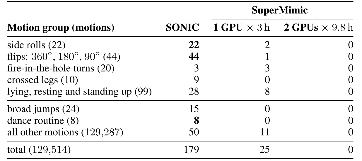
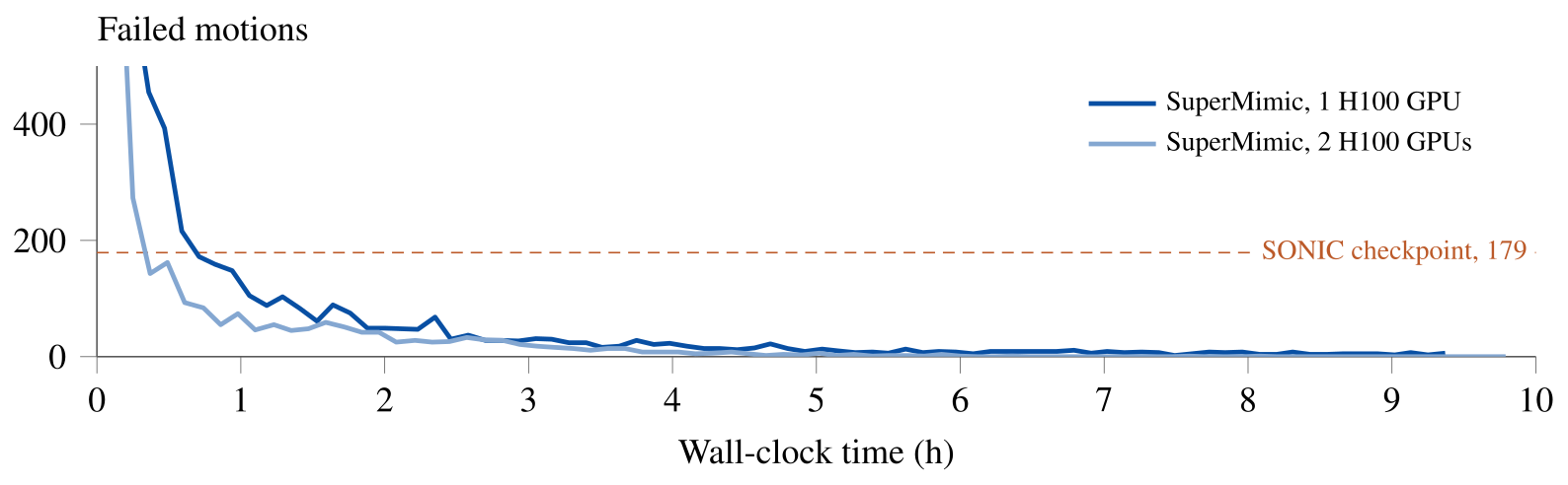
Three hours on one H100 surpasses the released SONIC checkpoint’s normalized return and reduces failed motions from 179 to 25 on a shared 129,514-motion benchmark. A two-H100 run reaches zero failures after 9.8 hours. These are deterministic evaluations of training-motion coverage. The headline GPU-hour ratio compares different hardware and training datasets; a separate LAFAN1 experiment supplies a more closely matched PPO comparison.
1. Introduction
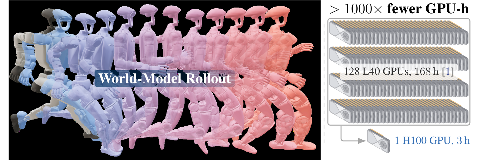
Large motion libraries share one robot’s body and contact dynamics. SuperMimic seeks to learn that shared structure once and reuse it for policy improvement across many reference motions. Figure 1 illustrates the learned-model rollout and reported training budgets.
The central tradeoff is fast, differentiable prediction in place of fresh simulator rollouts for every policy update. Its gradient is exact for the learned surrogate objective, not necessarily for the original simulator or physical robot.
Contributions
The paper combines an online learned world model, short-horizon actor–critic updates, a motion-library scaling study, physical Unitree G1 demonstrations, and a preliminary velocity-command interface. The evidence concerns the studied flat-ground motion-tracking setting.
Reusable motion representations and downstream control
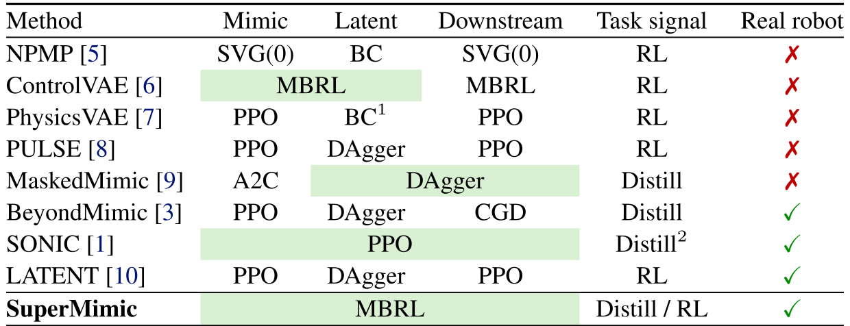
Table 1 retains every method, merged training stage, footnote, and deployment marker. SuperMimic shares a decoder across goal encoders, allowing a downstream interface to optimize either motion tracking or its own task reward. Joint training and gradient routing differ between methods; the table is an architectural comparison, not a common-benchmark ranking.
3. Method
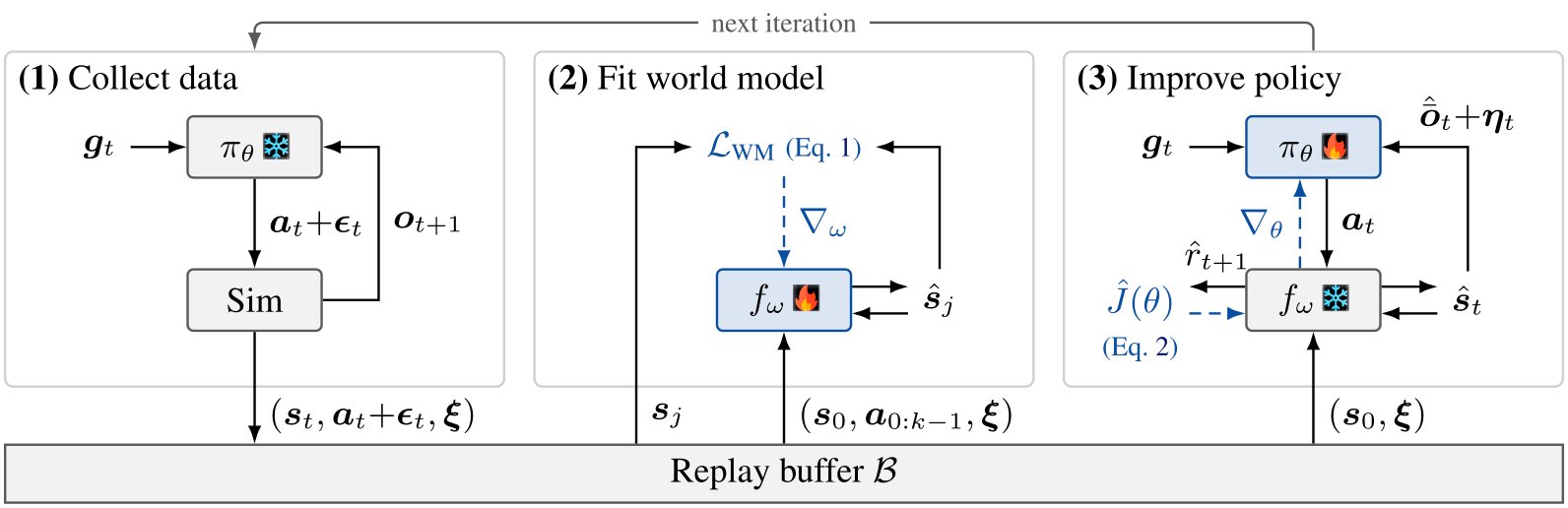
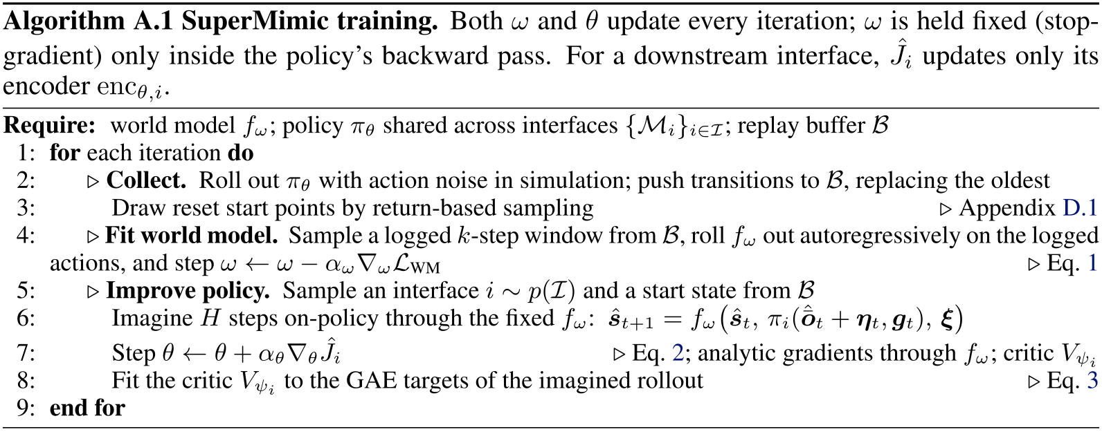
Training alternates simulator data collection, world-model fitting, and actor–critic optimization on imagined trajectories. Appendix D retains the complete algorithm.
3.1 SuperMimic training loop
The current deterministic policy collects simulator transitions into a fixed-size replay buffer. Optional action noise broadens model-training coverage, and the buffer stores the executed noisy action. Short replay windows fit the world model; replay states then initialize imagined policy rollouts. Model weights are frozen only during each policy update.
The policy receives a proprioceptive observation and goal. Soft survival weights use c0=1 and ct+1=ct(1−dt+1), with objective J(θ)=E[∑t≥0γtctrt+1]. Simulator terminations are binary; model terminations are probabilities, keeping imagined survival differentiable. Observations factor as ot=ōt+ηt, with known sensor noise added outside the model.
3.2 Learning a differentiable world model
The deterministic model conditions on simulation context: friction, joint calibration offsets, and torso center-of-mass offsets. Its dynamics and reward, observation, and termination heads are retained below; individual heads may be learned or analytic.
Equation 1 fits eight-step autoregressive windows using state, reward, and noise-free observation errors plus termination cross-entropy. Analytically computed heads contribute no learned-head loss. Context information is available to the model during training; the deployed actor uses noisy proprioception and a goal.
Equations


3.3 Learning the policy through the world model
Equation 2 sums discounted rewards across 32 imagined steps and bootstraps with the critic at the horizon. Rollouts start from replay states with their recorded context, and sensor noise is reintroduced before policy inference. Backpropagation through the fixed world model supplies the actor gradient.
The model is trained on eight-step windows but used over longer imagined horizons. This gives useful gradients in the reported experiments; stable long rollouts are an empirical claim, not a bound on accumulated error.
Equation

Critic objective
Equation 3 preserves the critic loss and backward return recursion. The terminal target is the critic’s horizon estimate; targets stay fixed during the critic fit. Updates use imagined transitions and a GAE-style λ return [26].
The critic extends the policy objective beyond the imagination window. Similar nominal tracking scores without it can conceal worse recovery from disturbances.
Equation

4. Experimental results
Training uses MuJoCo Warp and H100 80 GB SXM5 GPUs. Normalized return is undiscounted episode reward divided by its maximum; early termination lowers it. The authors report stable training across several seeds but provide no seed-variation bands.
Checkpoint evaluation, training-episode return, imagined-step efficiency, and simulator throughput are different measurements. The figures retain their separate definitions and budgets.
4.1 Tracking and compute comparison
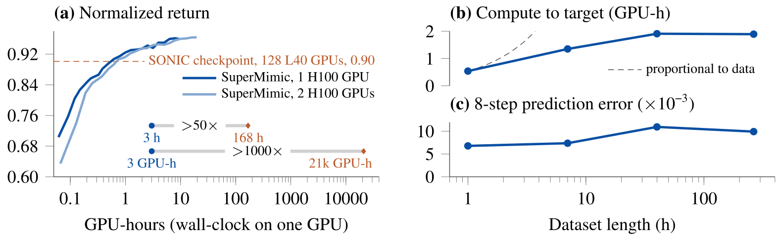
Figure 3 compares all checkpoints on the same 129,514 motions. After three hours on one H100, SuperMimic exceeds the released SONIC checkpoint’s 0.90 normalized return and has 25 failures versus 179. After 9.8 hours on two H100s, it has none under this protocol.
The three-hour threshold is chosen conservatively: later checkpoints maintain at least half the gap between SONIC and SuperMimic’s best result on both return and failure count. Appendix F defines the training-set benchmark and failure rule.
Compute accounting
SONIC’s reported 128 L40 GPUs for 168 hours total 21,504 GPU-hours, compared with three H100 GPU-hours. The approximate ratios are 7,200× in GPU-hours and 56× in elapsed time, summarized as over 1,000× and 50×. SuperMimic’s time includes data collection, model fitting, and policy updates; post-training checkpoint evaluation is excluded.
The training data also differs: 264.56 hours of public BONES-SEED for SuperMimic versus SONIC’s 611 hours. GPU-hours do not normalize hardware capability or utilization. The paper discusses peak throughput differences, but this remains a system-level comparison rather than an isolated algorithm-only speedup.
Controlled PPO-Sim comparison
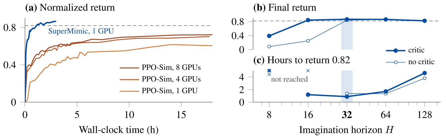
On LAFAN1’s forty clips, PPO-Sim shares the motions, observations, reward, termination, randomization, network sizes, and evaluation protocol. It uses BeyondMimic PPO hyperparameters and twice as many simulator environments per GPU.
SuperMimic reaches evaluation return 0.82 within 1.2 hours on one GPU. At the eighteen-hour budget, PPO-Sim reaches 0.60, 0.70, and 0.72 with one, four, and eight GPUs. Figure 4 also retains a separate horizon ablation based on training return, whose reset distribution changes during learning and differs from checkpoint evaluation.
4.2 Properties of the learned world model
Three analyses examine model accuracy across data sizes, simulation versus imagination throughput, and analytic updates versus PPO on imagined data.
Shared dynamics across the motion library
Across one, seven, forty, and 264 hours of motion, eight-step normalized state prediction error stays between 0.007 and 0.011, while compute to the target return grows slowly. The error is measured online on policy rollouts, not on an independently fixed held-out state distribution. The result supports reuse of one body’s dynamics within this sweep.
Imagination rollout speed
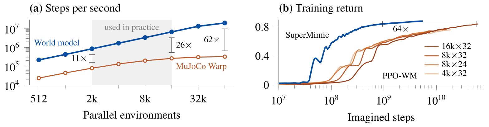
On one H100, model rollouts exceed MuJoCo Warp throughput by more than 10× over practical batches of 2,000–16,000 environments and by 62× at 64,000. A step is one 50 Hz control interval; the simulator computes four 5 ms physics substeps while the learned model runs at training TF32 precision. This is rollout throughput, not the whole training loop’s speedup.
Analytic gradients
On LAFAN1 walking, running, and sprinting motions, analytic actor–critic training reaches the best PPO-on-world-model training return with about 64× fewer imagined steps. Figure 5 keeps all four PPO batch configurations. This mechanism ablation isolates the update route more closely than the external SONIC comparison.
4.3 Critic, horizon, and recovery
The critic makes a sixteen-step horizon comparable to a critic-free thirty-two-step horizon. The default thirty-two-step version reaches training return 0.82 fastest; increasing the horizon from sixty-four to 128 nearly triples time and reduces final return.
Under simulated T-pose velocity pushes of 0.5–4 m/s, the critic policy settles in 0.5–2.4 seconds. The critic-free policy continues stumbling even at 0.5 m/s and falls at 4 m/s. These are simulator perturbation results, separate from the physical demonstrations.
4.4 Real-robot transfer
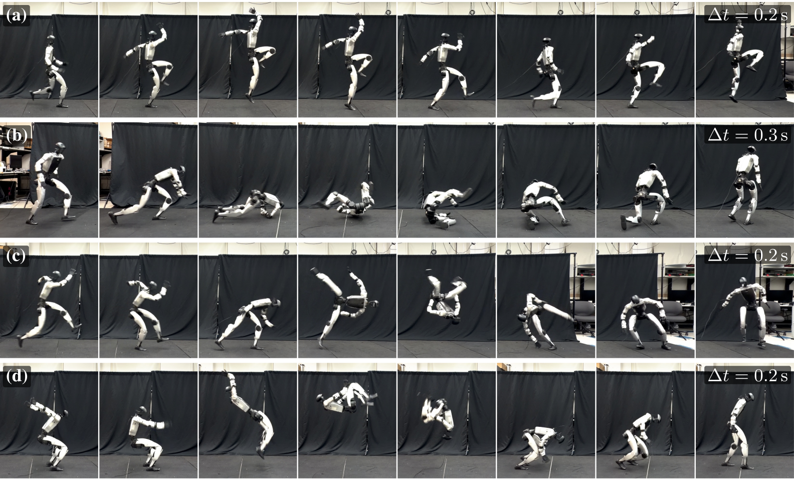
Figure 6 retains complete frame sequences for a skipping jump, side roll, 90° flip, and in-place 360° flip on a physical Unitree G1. One general tracker is used without per-motion tuning. The paper gives qualitative demonstrations rather than repeated-trial success rates or a physical comparison with SONIC.
4.5 Downstream task interfaces
A velocity encoder trained on its own task reward is compared with one trained through the motion-tracking objective using commands derived from demonstrations. Both share a learned world model and motion decoder; this preliminary experiment is detailed in Appendix G.
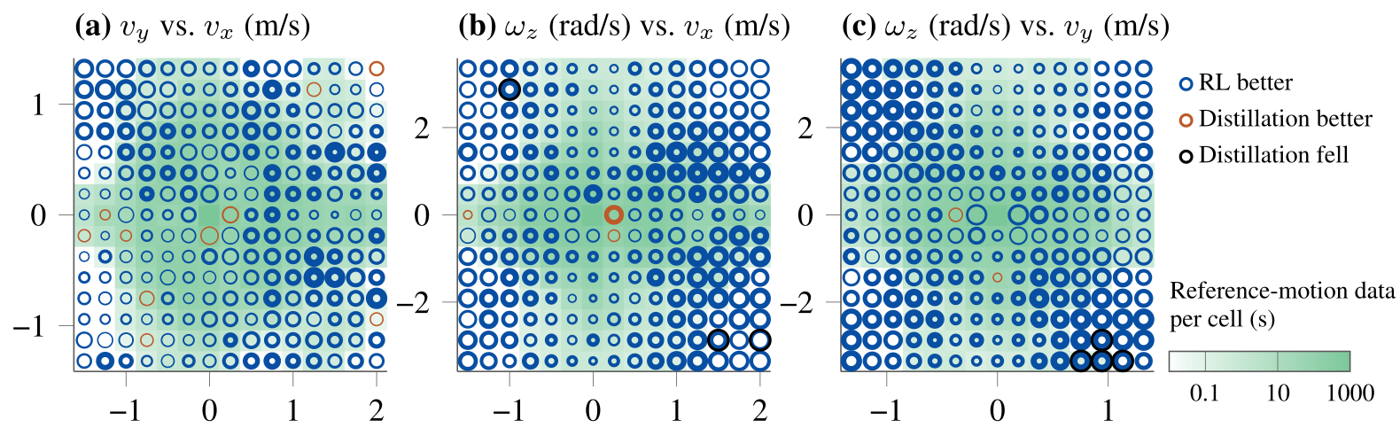
Figure 7 retains the command grids, error-size encoding, fall markers, and reference-data density. Task-specific reward training generally improves step-response accuracy, especially outside well-covered reference velocities.
5. Conclusion
The experiments show substantial training-cost reductions for flat-ground humanoid motion tracking and useful physical transfer. They support the proposed roles of shared learned dynamics, fast rollouts, and analytic gradients. The broad claim that compute ceases to be a bottleneck is limited by the tested robot, tasks, data range, and hardware.
6. Limitations and future work
The world model learns only from simulator transitions, and training excludes terrain and object interaction. Whether real data improves the model or supports system identification remains open.
The downstream velocity reward updates only its encoder, with decoder weights frozen for that gradient. The benefit of concurrent interface training is untested; joint optimization of the shared decoder on downstream rewards is future work.
Acknowledgments
The authors acknowledge collaborators, support from Komatsu, the BAIR Center for Humanoid Intelligence, Apple, and the RAI Institute, compute from Lambda, and Bones Studio motion data. Abbeel and Sreenath also hold Amazon Scholar appointments; the paper identifies the work as UC Berkeley research unaffiliated with Amazon.
A. Observation, action, reward, and context
Appendix A specifies the deployed policy inputs, goals and actions, tracking reward, termination, and model-training context.
Observation
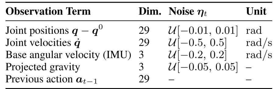
Table A.1 retains all 93 per-frame observation dimensions and their sensor-noise ranges: joint positions and velocities, base angular velocity, projected gravity, and previous action. The actor receives ten observation frames.
Goal
The motion encoder receives ten future reference frames, extending BeyondMimic’s single-frame target. Other goal interfaces replace the reference with their command representation.
Action
The normalized action maps to joint setpoint qsp=αat+q0. Low proportional-derivative gains make this a torque-related control proxy rather than strict position tracking.
Reward
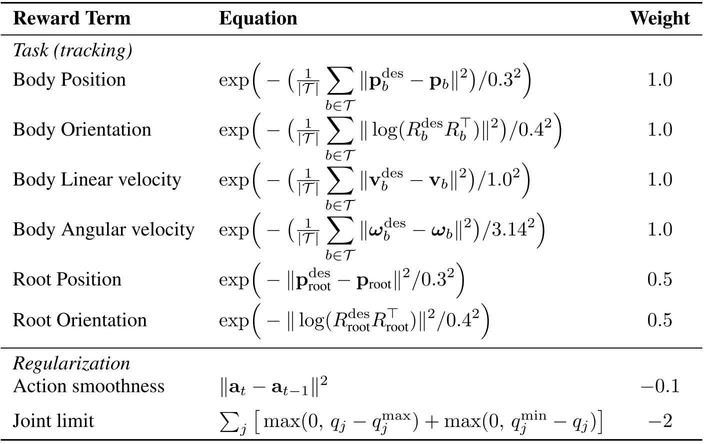
Table A.2 preserves every tracking and regularization formula and weight. SuperMimic removes BeyondMimic’s self-collision penalty and lowers the joint-limit penalty from −10 to −2. The authors argue the self-contact exploit addressed by that penalty has no benefit for their deterministic imagined policy.
Termination
Tracking terminates if root height error exceeds 0.25 m or the absolute difference in reference/robot gravity-direction z-components exceeds 0.8. For an upright reference, the latter corresponds to about 78° tilt. End-effector deviation does not terminate an episode.
Simulation context and randomization
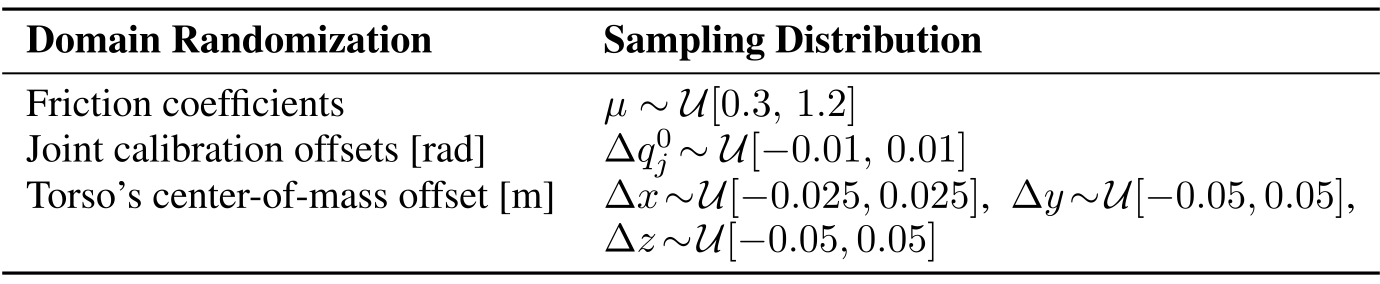
Table A.3 retains friction, joint-offset, and torso center-of-mass sampling ranges. Unlike BeyondMimic, training omits root-velocity pushes because those abrupt state changes are not represented by this deterministic model. Physical-parameter randomization is reported sufficient for the demonstrated hardware transfer.
B. Joint training across goal interfaces
Equation A.1 defines per-interface encoders and a shared decoder. Each interface has its own goals, reward, termination, and critic, while all share the body-dynamics model. The lifted objective is maxθEi∼p(I)[Ĵi(θ)].
Downstream gradients pass through the decoder to the selected encoder, but stop at the decoder’s weights. Motion-tracking updates still train the decoder. The velocity encoder additionally uses an observation-history feature and latent alignment on reference-command rollouts.
Equation

C. Network architectures
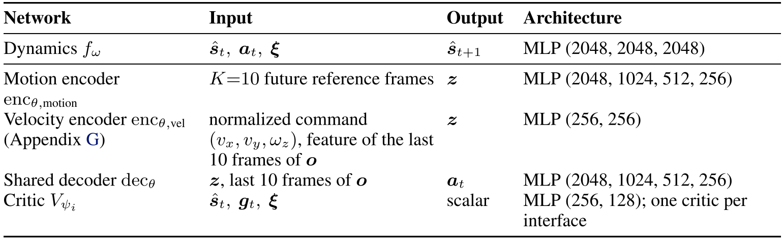
Table A.4 retains every input, output, and hidden width. The dynamics MLP has three 2,048-unit layers; the shared policy latent has 32 dimensions bounded by tanh. Motion and velocity encoders have different input structures and capacities.
D. Training loop and hyperparameters
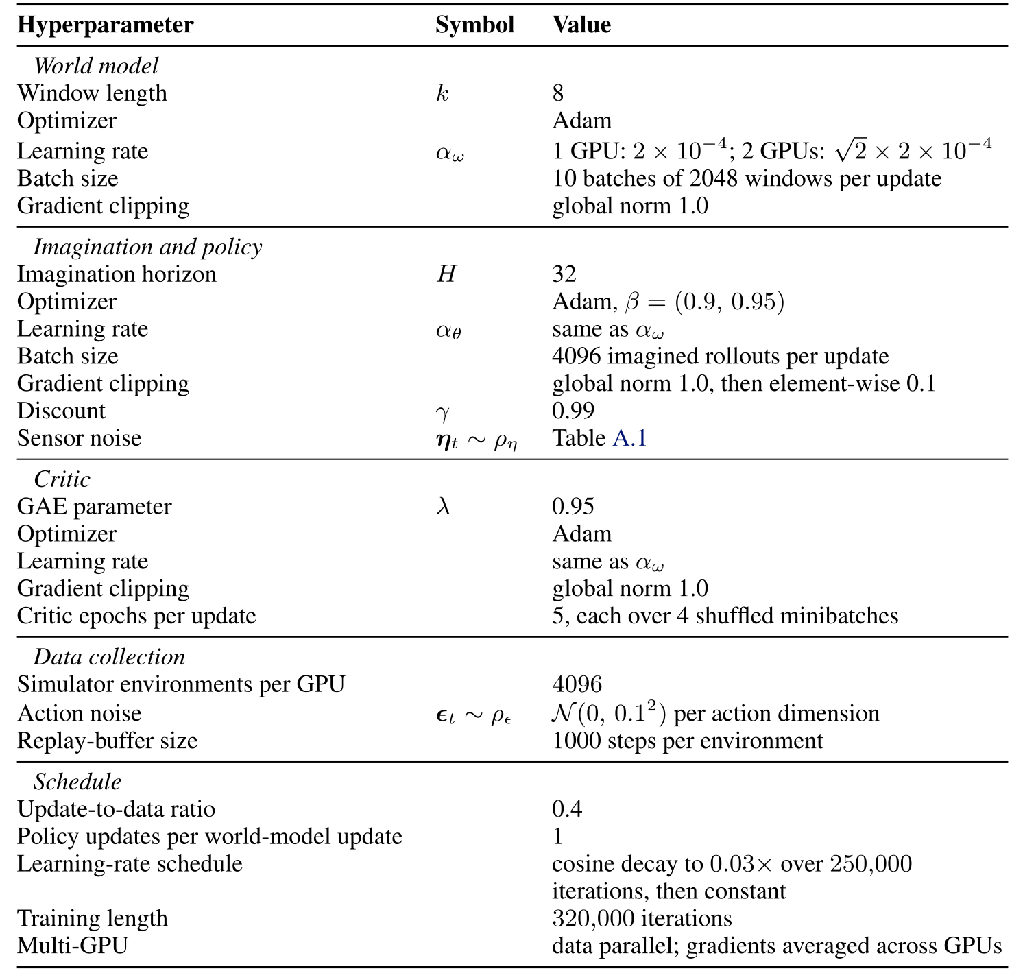
Appendix D retains the full nine-step training algorithm and hyperparameters for the one- and two-GPU runs.
D.1 Algorithm
Algorithm A.1 preserves data collection, reset sampling, autoregressive model fitting, interface selection, imagined rollout, actor update, and critic fitting. The model updates each iteration and is held fixed only for policy backpropagation.
Return-based reset sampling
Resets use one-second motion bins with running discounted returns. The mixture is 50% uniform, 40% softmaxb(−25Gb/Gmax), and 10% proportional to past softmax weights. This emphasizes difficult motion regions while retaining practice after improvement.
D.2 Hyperparameters
Table A.5 retains all optimizer, batch, clipping, noise, buffer, schedule, and parallel-training settings. Defaults include eight-step model windows, thirty-two-step imagination, discount 0.99, GAE λ=0.95, 4,096 environments per GPU, and 1,000 buffered steps per environment. The two-GPU learning rate is √2 times the one-GPU rate.
E. Motion data filtering
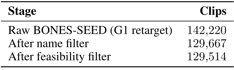
The public G1-retargeted BONES-SEED release has 142,220 clips. Filtering removes terrain/object interactions and infeasible retargets, leaving 129,514 clips. Table A.7 retains counts after each pass; the benchmark therefore excludes some behaviors unavailable to a free-standing flat-ground robot.
Name filter
Action-name keywords remove 12,553 clips, including stairs, ladders, boxes, chairs, sitting, climbing, and specified raised-support actions. The list adapts SONIC’s public processing code and adds missed terms.
Feasibility filter
Forward kinematics removes another 153 clips. Criteria include a lowest body-link height above 0.20 m for at least 0.6 s; below −0.12 m at any time or below −0.08 m for over 80% of a clip; and both feet more than 0.02 m above the floor for at least 0.5 s while upright, at standing height, and nearly stationary.
The floating-feet test uses geometry-to-plane distance and excludes ballistic jumps through its stationary gate. These thresholds are tuned for the G1 retarget at 50 Hz.
F. Evaluation
Appendix F defines the common simulation, failure rule, full motion-group counts, and dataset-size sweep.
F.1 Benchmark metrics
Each of the 129,514 training motions is run once from its first frame with friction 1.0, deterministic physics, no domain randomization, and no observation noise. Policies retain their own actuator gains, action scales, and observation construction.
Failure uses SuperMimic’s root-height/tilt termination. SONIC’s original criterion instead checks root and end-effector height without an orientation term. Thus zero failures describes this shared deterministic training-set protocol, not unseen-motion generalization or a reliability guarantee.
F.2 Failed motions
Table A.8 retains every motion group. SONIC’s released checkpoint fails all 44 flips, all 22 side rolls, and all eight dance-routine clips, totaling 179 failures. Its separate v1.1 checkpoint has 239 failures. SuperMimic has 25 after three hours on one GPU and none after 9.8 hours on two.
Figure A.1 retains failure counts across saved checkpoints, evaluated every 4,000 iterations. The hardest five listed groups contain fourteen of the twenty-five early SuperMimic failures.
F.3 Experiment protocols
The dataset-length sweep uses one, seven, forty, and 264 hours from the filtered BONES-SEED set. The shared benchmark in Figure 3 uses the complete filtered training-motion set.
G. Velocity-command task
Appendix G gives the complete separate experiment for velocity-command encoders.
G.1 Training setup
Each encoder is trained from scratch in its own 100,000-iteration run, together with the motion interface, using walking/running clips from LAFAN1 and BONES-SEED. Half of simulator environments and each imagined batch use the velocity interface. This mixed-batch implementation differs from Algorithm A.1’s single sampled interface per update.
Commands
Commands specify heading-frame forward/lateral velocity and world-frame yaw rate. Reference commands use a centered twenty-five-frame velocity mean. The RL run resamples command source every reset and every five seconds: half reference-derived, half uniform over vx∈[−1.5,2] m/s, vy∈[−1.32,1.32] m/s, and ωz∈[−3.35,3.35] rad/s. Uniform commands become standing with probability 0.1.
Encoder
On reference-command rollouts, a mean-squared latent-alignment loss of weight 0.1 pulls the velocity latent toward a stop-gradient motion latent.
Rollouts, reward, and termination
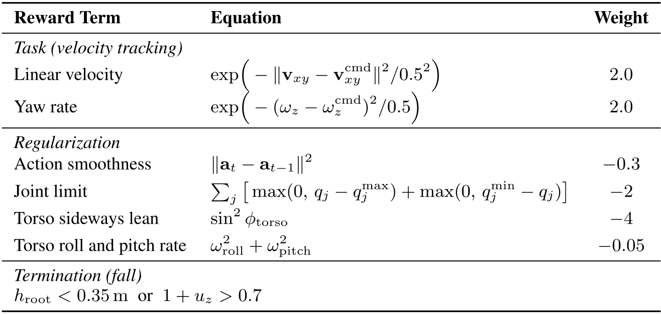
Each interface starts imagination from its own logged states. The RL encoder uses the velocity reward and fall-only termination in Table A.6; distillation uses the tracking reward and termination. All terms in both reward tables are multiplied by the 0.02-second control period.
G.2 Step test
From standing, each command is held for five seconds in four trials. Relative steady-state error is the norm of mean velocity error over the last two seconds divided by command norm. The reported per-command value is the median among non-falling trials.
Three fifteen-by-fifteen command planes, excluding standing, supply 672 responses. Figure 7 caps errors at 0.9 and places a policy at the cap when all four trials fall.
Results
The RL encoder has lower error on 650 responses and distillation on fifteen; distillation falls in all four trials on seven fast-turn commands. Median relative errors are 0.16 and 0.49. These runs have one training seed each, and error statistics condition on surviving trials.