Literature
Display
← All papers

Noise-Invariant Spatial Encoding for 3D Manipulation Policies under Depth Corruption

Zhiyuan Yang · Jiaju He · Ruiteng Zhao · Anqi Cheng · Haiyue Zhu · Kezhi Mao

Preprint posted · CoRL 2026 (accepted) ↗

Robotics10 min text · CondensedOriginal paper ↗
Contents

Overview

This edition covers the full 22-page paper and Appendices A–J. Every figure/table panel, equation, caption, reference and original paired RGB/depth demonstration remains. Native PDF layouts restore fine chart labels and table formatting while retaining selectable original values/notation. Haiyue Zhu and Kezhi Mao are corresponding authors. The clean-depth training target used for single-view MetaWorld is distinguished from the noisy cross-view targets used for RLBench and the real-robot motivation.

At a glance

Depth errors become incorrect token positions in 3D manipulation policies. NISE combines training-only Geometric Cross-View Self-Supervision (GCVSS) with deployed Gaussian Marginalized 3D Attention (GM3A). On the reported noisy-trained RLBench setting it scores 89.0/85.7/84.1% for clean/mild/saturated depth; MetaWorld scores 79.0/78.2/77.4%. A strong geometry-pretrained backbone supplies part of the advantage, so within-stack ablations matter. Five real tasks use thirty trials per method. ‘Noise invariant’ means lower measured representation drift, not mathematically identical features or immunity to systematic depth error.

1 Introduction

A depth-lifted policy uses metric distances and reachability, but missing values, edge artifacts and wrong surfaces corrupt those coordinates before action prediction. Matched noisy training helps without fully removing the error. NISE targets the learned spatial interface: cross-view consistency shapes features, and position-uncertainty attenuation changes how attention uses them. Figure 1’s saturated task-mean gaps over the strongest listed baseline are about 33.2 RLBench and 40.2 MetaWorld percentage points.
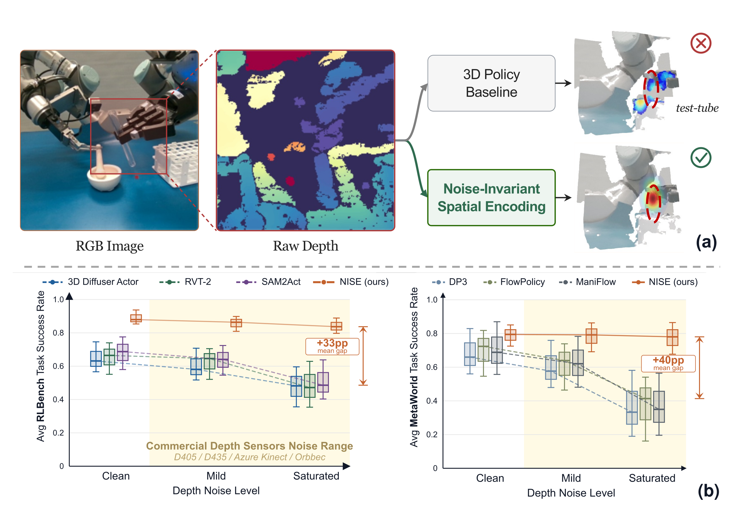
Complete original Figure 1: Realistic depth corruption breaks what 3D policies can trust. (a) In a transparent test-tube manipulation scene, raw depth contains missing and geometrically wrong measurements; a standard 3D policy consumes this corrupted geometry as exact and fails, while NISE succeeds. (b) Depth-noise robustness on RLBench PerAct-18 [ 1 , 2 ] and MetaWorld [ 3 ] . NISE maintains higher success rates as depth corruption increases, with a smaller clean-to-saturated decline than the compared baselines.
Figure 1: Realistic depth corruption breaks what 3D policies can trust. (a) In a transparent test-tube manipulation scene, raw depth contains missing and geometrically wrong measurements; a standard 3D policy consumes this corrupted geometry as exact and fails, while NISE succeeds. (b) Depth-noise robustness on RLBench PerAct-18 [1, 2] and MetaWorld [3]. NISE maintains higher success rates as depth corruption increases, with a smaller clean-to-saturated decline than the compared baselines.

2 Related Work

Point-cloud, voxel, virtual-view and depth-lifted-token policies all depend on geometry. Depth repair and geometry-pretrained backbones improve inputs/features, while related representation methods also address uncertainty or consistency. NISE’s claim is their specific combination of cross-view feature supervision and adaptive rotary-position attenuation. The experiments explicitly include strong-backbone and repair controls, rather than attributing every cross-architecture gap to these two mechanisms.

3 NISE : Noise-Invariant Spatial Encoding

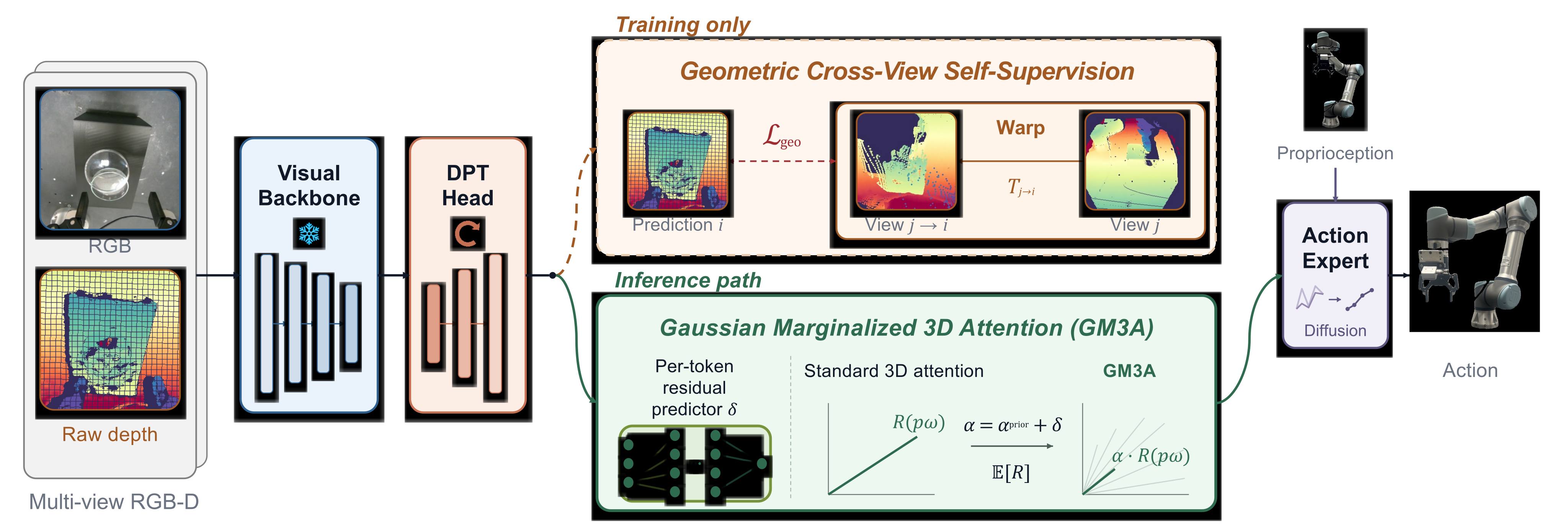
The design has a shared trainable spatial feature map above a frozen visual backbone. During training a geometry decoder predicts a calibrated, visibility-filtered cross-view target. At deployment that decoder disappears; adaptive positional attenuation stays inside the action policy.

3.1 From Depth Noise to Action Error

Back-projecting noisy depth through camera calibration turns each depth perturbation into a coordinate error, mainly along its camera ray. Rotary phases and cross-camera spatial relations then inherit that error. The complete observation, corruption, lifting and feature definitions remain. This is a failure-channel argument, rather than a universal quantitative bound from depth noise to action failure.

Equations
𝒪rgbd={Iv,Dv,Kv,Tv}v=1V,a=πθ​(𝒪rgbd,𝐬prop).\mathcal{O}_{\text{rgbd}}={\{I^{v},\,D^{v},\,K^{v},\,T^{v}\}}_{v=1}^{V},\qquad a=\pi_{\theta}(\mathcal{O}_{\text{rgbd}},\,\mathbf{s}_{\text{prop}}).
D~v=Dv+ϵv,\tilde{D}^{v}=D^{v}+\epsilon^{v},
𝐩⁡(u,v)=D~​(u,v)⋅K−1​[u,v, 1]⊤,\mathbf{p}(u,v)\;=\;\tilde{D}(u,v)\cdot K^{-1}{[\,u,\,v,\,1\,]}^{\top},
zi=fθ​(Iv,D~v,𝐩i)z_{i}\;=\;f_{\theta}\big(I^{v},\,\tilde{D}^{v},\,\mathbf{p}_{i}\big)
Complete original Figure 2: NISE framework. Per-camera RGB-D is encoded by a frozen visual backbone ViT and a trainable DPT-style head [ 21 ] into a shared spatial feature map. NISE acts on this shared map: during training, Geometric Cross-View Self-Supervision attaches a cross-view geometry head to encourage view-consistent geometry in the same features consumed by the policy; at deployment, this head is removed.
Gaussian Marginalized 3D Attention remains in the deployed policy and carries per-token coordinate uncertainty into 3D attention, so lifted tokens influence action features according to their spatial reliability.
Figure 2: NISE framework. Per-camera RGB-D is encoded by a frozen visual backbone ViT and a trainable DPT-style head [21] into a shared spatial feature map. NISE acts on this shared map: during training, Geometric Cross-View Self-Supervision attaches a cross-view geometry head to encourage view-consistent geometry in the same features consumed by the policy; at deployment, this head is removed. Gaussian Marginalized 3D Attention remains in the deployed policy and carries per-token coordinate uncertainty into 3D attention, so lifted tokens influence action features according to their spatial reliability.

3.2 Geometric Cross-View Self-Supervision

For a target view, source depth is forward-warped with calibrated intrinsics/extrinsics, z-buffered and filtered for valid visible splats. A masked L1 loss trains a geometry head on the shared policy features. The target is still noisy; the Noise2Noise analogy does not impose independent unbiased noise across camera views. Multiple views that agree on the same background through a transparent object can supply a consistent but wrong target. The geometry head supervises representation learning rather than preprocessing deployed depth.

Equations
𝐱i∼Ki​Ti←j​(dj​(𝐱j)​Kj−1​𝐱¯j),dj→i​(𝐱i)=[Ti←j​(dj​(𝐱j)​Kj−1​𝐱¯j)]z.\mathbf{x}_{i}\sim K_{i}T_{i\leftarrow j}\left(d_{j}(\mathbf{x}_{j})K_{j}^{-1}\bar{\mathbf{x}}_{j}\right),\qquad d_{j\rightarrow i}(\mathbf{x}_{i})={\left[T_{i\leftarrow j}\left(d_{j}(\mathbf{x}_{j})K_{j}^{-1}\bar{\mathbf{x}}_{j}\right)\right]}_{z}.
D^i=gϕ​(𝐅i),ℒgeo=1|Mj→i|​∑𝐱∈Mj→i|D^i​(𝐱)−dj→i​(𝐱)|.\widehat{D}_{i}=g_{\phi}(\mathbf{F}_{i}),\qquad\mathcal{L}_{\mathrm{geo}}=\frac{1}{|M_{j\rightarrow i}|}\sum_{\mathbf{x}\in M_{j\rightarrow i}}\left|\widehat{D}_{i}(\mathbf{x})-d_{j\rightarrow i}(\mathbf{x})\right|.

3.3 Gaussian Marginalized 3D Attention

For locally Gaussian coordinate uncertainty, the exact sinusoidal moment is the mean phase times exp(−variance·frequency²/2). Larger uncertainty attenuates high frequencies more. Per-token/per-axis/per-band residuals then adapt that prior under an L2 anchor. The analytic moment concerns positional features, not an exact expectation of the full nonlinear attention output. Once learned residuals are added, coefficients need not equal a Gaussian marginal; the manuscript does not specify a clamp guaranteeing every learned coefficient stays in [0,1]. Biased or multimodal wrong-surface errors also exceed the local Gaussian approximation.

Equations
𝔼⁡[ei​ωk​p~a]=ei​ωk​μa​exp(−σa2ωk2/2)⏟αk,aprior,\mathbb{E}\!\left[e^{\mathrm{i}\omega_{k}\tilde{p}_{a}}\right]=e^{\mathrm{i}\omega_{k}\mu_{a}}\underbrace{\exp\!\big(-\sigma_{a}^{2}\omega_{k}^{2}/2\big)}_{\alpha^{\text{prior}}_{k,a}},
αk,a=αk,aprior+δk,a,ℒreg=𝔼token,k,a​[(αk,a−αk,aprior)2].\alpha_{k,a}=\alpha^{\text{prior}}_{k,a}+\delta_{k,a},\qquad\mathcal{L}_{\text{reg}}=\mathbb{E}_{\text{token},k,a}\!\left[{(\alpha_{k,a}-\alpha^{\text{prior}}_{k,a})}^{2}\right].

3.4 Training and Deployment

Total training loss combines the base action objective, geometry loss weighted .1 and prior regularizer weighted 1.0. Deployment removes the geometry decoder, keeping the frozen backbone, shared feature aggregator, GM3A and native action expert. No additional cross-view reconstruction branch or clean-depth input is required at inference.

Equation
ℒtotal=ℒpolicy+λgeo​ℒgeo+λreg​ℒreg\mathcal{L}_{\text{total}}=\mathcal{L}_{\text{policy}}+\lambda_{\text{geo}}\,\mathcal{L}_{\text{geo}}+\lambda_{\text{reg}}\,\mathcal{L}_{\text{reg}}

4 Experiments

Experiments test noise robustness, clean-depth retention, physical manipulation, component attribution, repair complementarity and representation diagnostics. Baselines retain their own architectures; same-stack controls provide the more direct mechanism comparison.

4.1 Setup

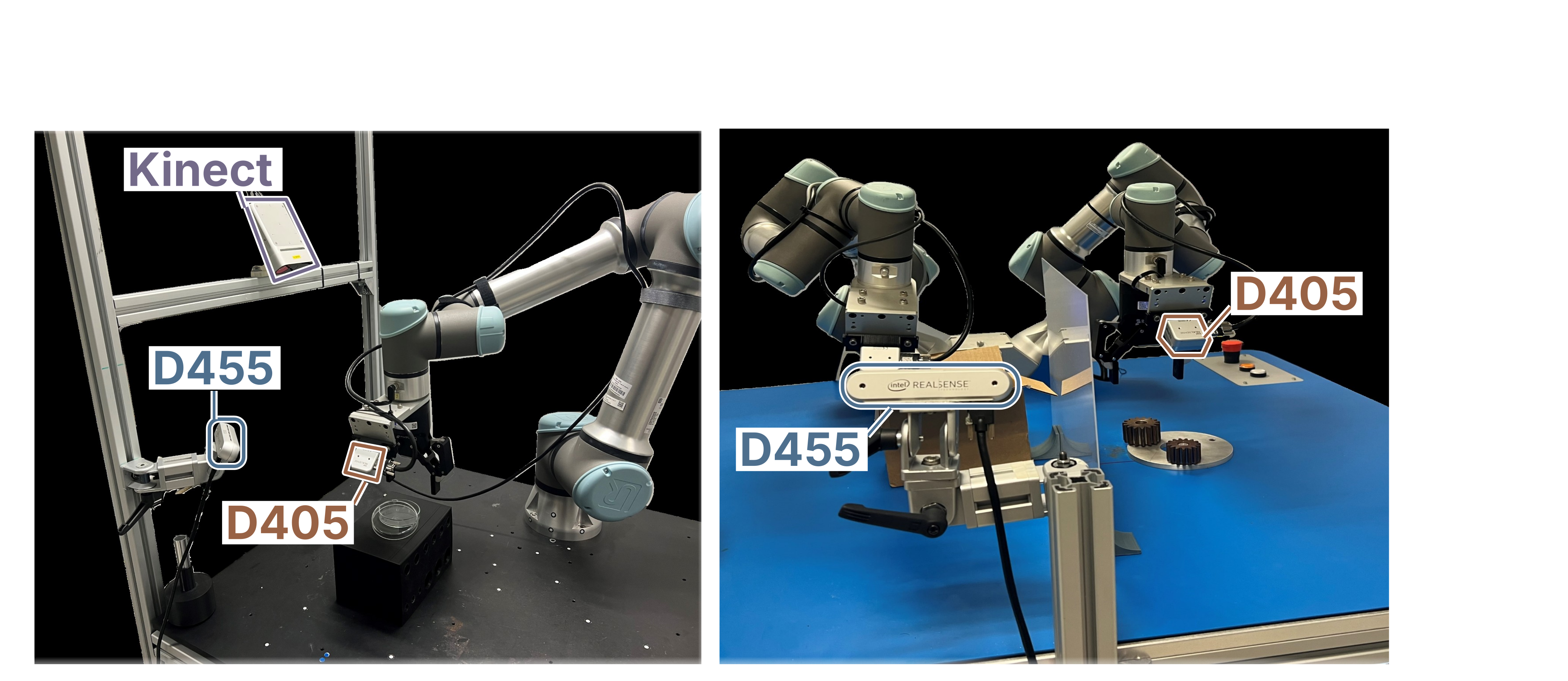
A common dataloader wrapper adds range/disparity noise, edge dropout, holes and displaced lookup. Clean, mild and saturated levels are sampled equally in the controlled noisy-training comparison; Table 2 averages three independent training runs, with 25 episodes per condition. Real methods share demonstrations/raw streams but use their own tuned protocols. Crucially, four-view RLBench uses noisy cross-view supervision, while single-view MetaWorld uses clean simulator depth as its auxiliary training target. Calibration is described for D405/Azure Kinect; the visible sensor names do not establish exhaustive calibration of every commodity camera.
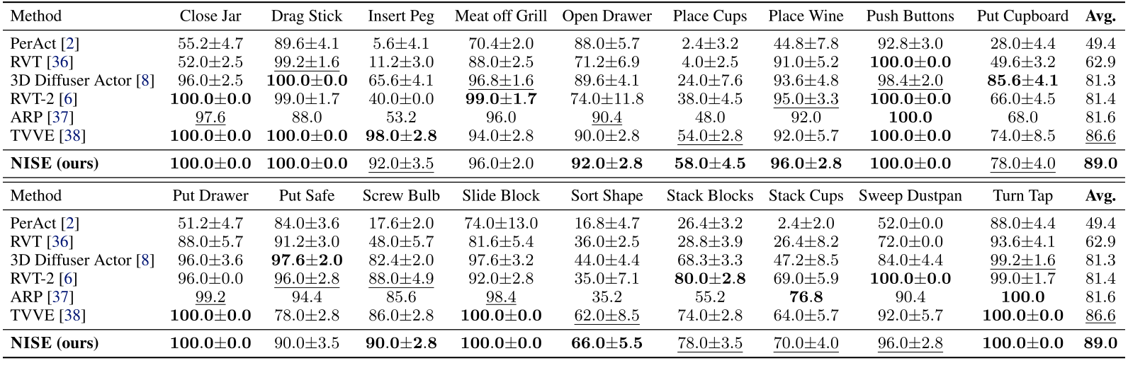
Complete original Table 1: Quantitative results on RLBench PerAct-18. Per-task success rates (%, mean ± \pm standard deviation where available) on the standard 18-task PerAct suite under clean-depth evaluation. NISE reports mean ± \pm standard deviation over repeated evaluations of a fixed checkpoint.
Published baselines use clean-depth training, while NISE uses noisy-depth training.
The best and second-best distinct means per column are bold and underlined, respectively, including ties.
Table 1: Quantitative results on RLBench PerAct-18. Per-task success rates (%, mean ±\pm standard deviation where available) on the standard 18-task PerAct suite under clean-depth evaluation. NISE reports mean ±\pm standard deviation over repeated evaluations of a fixed checkpoint. Published baselines use clean-depth training, while NISE uses noisy-depth training. The best and second-best distinct means per column are bold and underlined, respectively, including ties.
Accessible table, original values and citation links
Method Close Jar Drag Stick Insert Peg Meat off Grill Open Drawer Place Cups Place Wine Push Buttons Put Cupboard Avg.
PerAct [2] 55.2±4.755.2{\pm}4.7 89.6±4.189.6{\pm}4.1 5.6±4.15.6{\pm}4.1 70.4±2.070.4{\pm}2.0 88.0±5.788.0{\pm}5.7 2.4±3.22.4{\pm}3.2 44.8±7.844.8{\pm}7.8 92.8±3.092.8{\pm}3.0 28.0±4.428.0{\pm}4.4 49.449.4
RVT [36] 52.0±2.552.0{\pm}2.5 99.2±1.6¯\underline{99.2{\pm}1.6} 11.2±3.011.2{\pm}3.0 88.0±2.588.0{\pm}2.5 71.2±6.971.2{\pm}6.9 4.0±2.54.0{\pm}2.5 91.0±5.291.0{\pm}5.2 100.0±0.0\mathbf{100.0{\pm}0.0} 49.6±3.249.6{\pm}3.2 62.962.9
3D Diffuser Actor [8] 96.0±2.596.0{\pm}2.5 100.0±0.0\mathbf{100.0{\pm}0.0} 65.6±4.165.6{\pm}4.1 96.8±1.6¯\underline{96.8{\pm}1.6} 89.6±4.189.6{\pm}4.1 24.0±7.624.0{\pm}7.6 93.6±4.893.6{\pm}4.8 98.4±2.0¯\underline{98.4{\pm}2.0} 85.6±4.1\mathbf{85.6{\pm}4.1} 81.381.3
RVT-2 [6] 100.0±0.0\mathbf{100.0{\pm}0.0} 99.0±1.799.0{\pm}1.7 40.0±0.040.0{\pm}0.0 99.0±1.7\mathbf{99.0{\pm}1.7} 74.0±11.874.0{\pm}11.8 38.0±4.538.0{\pm}4.5 95.0±3.3¯\underline{95.0{\pm}3.3} 100.0±0.0\mathbf{100.0{\pm}0.0} 66.0±4.566.0{\pm}4.5 81.481.4
ARP [37] 97.6¯\underline{97.6} 88.088.0 53.253.2 96.096.0 90.4¯\underline{90.4} 48.048.0 92.092.0 100.0\mathbf{100.0} 68.068.0 81.681.6
TVVE [38] 100.0±0.0\mathbf{100.0{\pm}0.0} 100.0±0.0\mathbf{100.0{\pm}0.0} 98.0±2.8\mathbf{98.0{\pm}2.8} 94.0±2.894.0{\pm}2.8 90.0±2.890.0{\pm}2.8 54.0±2.8¯\underline{54.0{\pm}2.8} 92.0±5.792.0{\pm}5.7 100.0±0.0\mathbf{100.0{\pm}0.0} 74.0±8.574.0{\pm}8.5 86.6¯\underline{86.6}
NISE (ours) 100.0±0.0\mathbf{100.0{\pm}0.0} 100.0±0.0\mathbf{100.0{\pm}0.0} 92.0±3.5¯\underline{92.0{\pm}3.5} 96.0±2.096.0{\pm}2.0 92.0±2.8\mathbf{92.0{\pm}2.8} 58.0±4.5\mathbf{58.0{\pm}4.5} 96.0±2.8\mathbf{96.0{\pm}2.8} 100.0±0.0\mathbf{100.0{\pm}0.0} 78.0±4.0¯\underline{78.0{\pm}4.0} 89.0\mathbf{89.0}
Method Put Drawer Put Safe Screw Bulb Slide Block Sort Shape Stack Blocks Stack Cups Sweep Dustpan Turn Tap Avg.
PerAct [2] 51.2±4.751.2{\pm}4.7 84.0±3.684.0{\pm}3.6 17.6±2.017.6{\pm}2.0 74.0±13.074.0{\pm}13.0 16.8±4.716.8{\pm}4.7 26.4±3.226.4{\pm}3.2 2.4±2.02.4{\pm}2.0 52.0±0.052.0{\pm}0.0 88.0±4.488.0{\pm}4.4 49.449.4
RVT [36] 88.0±5.788.0{\pm}5.7 91.2±3.091.2{\pm}3.0 48.0±5.748.0{\pm}5.7 81.6±5.481.6{\pm}5.4 36.0±2.536.0{\pm}2.5 28.8±3.928.8{\pm}3.9 26.4±8.226.4{\pm}8.2 72.0±0.072.0{\pm}0.0 93.6±4.193.6{\pm}4.1 62.962.9
3D Diffuser Actor [8] 96.0±3.696.0{\pm}3.6 97.6±2.0\mathbf{97.6{\pm}2.0} 82.4±2.082.4{\pm}2.0 97.6±3.297.6{\pm}3.2 44.0±4.444.0{\pm}4.4 68.3±3.368.3{\pm}3.3 47.2±8.547.2{\pm}8.5 84.0±4.484.0{\pm}4.4 99.2±1.6¯\underline{99.2{\pm}1.6} 81.381.3
RVT-2 [6] 96.0±0.096.0{\pm}0.0 96.0±2.8¯\underline{96.0{\pm}2.8} 88.0±4.9¯\underline{88.0{\pm}4.9} 92.0±2.892.0{\pm}2.8 35.0±7.135.0{\pm}7.1 80.0±2.8\mathbf{80.0{\pm}2.8} 69.0±5.969.0{\pm}5.9 100.0±0.0\mathbf{100.0{\pm}0.0} 99.0±1.799.0{\pm}1.7 81.481.4
ARP [37] 99.2¯\underline{99.2} 94.494.4 85.685.6 98.4¯\underline{98.4} 35.235.2 55.255.2 76.8\mathbf{76.8} 90.490.4 100.0\mathbf{100.0} 81.681.6
TVVE [38] 100.0±0.0\mathbf{100.0{\pm}0.0} 78.0±2.878.0{\pm}2.8 86.0±2.886.0{\pm}2.8 100.0±0.0\mathbf{100.0{\pm}0.0} 62.0±8.5¯\underline{62.0{\pm}8.5} 74.0±2.874.0{\pm}2.8 64.0±5.764.0{\pm}5.7 92.0±5.792.0{\pm}5.7 100.0±0.0\mathbf{100.0{\pm}0.0} 86.6¯\underline{86.6}
NISE (ours) 100.0±0.0\mathbf{100.0{\pm}0.0} 90.0±3.590.0{\pm}3.5 90.0±2.8\mathbf{90.0{\pm}2.8} 100.0±0.0\mathbf{100.0{\pm}0.0} 66.0±5.5\mathbf{66.0{\pm}5.5} 78.0±3.5¯\underline{78.0{\pm}3.5} 70.0±4.0¯\underline{70.0{\pm}4.0} 96.0±2.8¯\underline{96.0{\pm}2.8} 100.0±0.0\mathbf{100.0{\pm}0.0} 89.0\mathbf{89.0}
Complete original Figure 3: Real-robot setup: single-arm UR5e (left) and bimanual UR3e (right). Camera labels identify Azure Kinect and RealSense D455/D405.
Figure 3: Real-robot setup: single-arm UR5e (left) and bimanual UR3e (right). Camera labels identify Azure Kinect and RealSense D455/D405.

4.2 Results

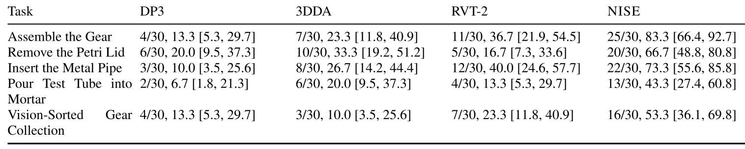
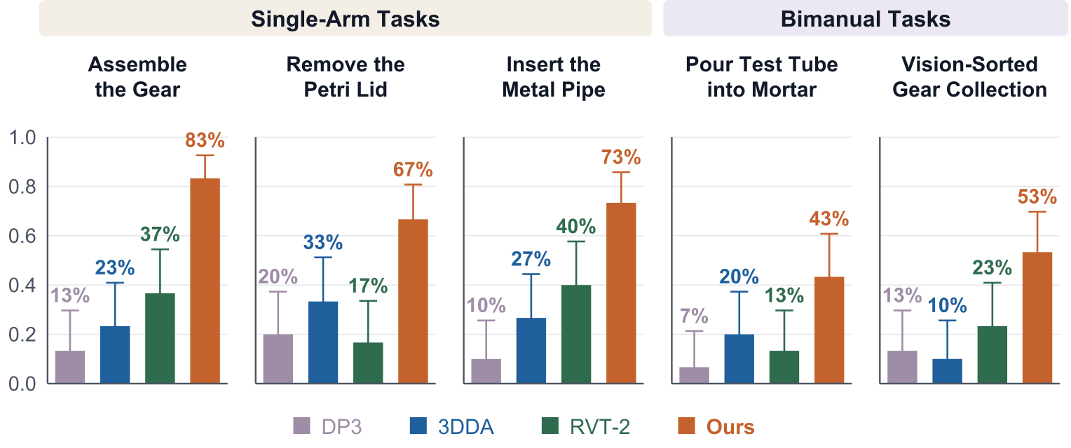
Table 1 compares NISE clean-input performance with published clean-trained baselines; its NISE deviations reflect repeated evaluations of a fixed checkpoint. Table 2 instead compares mixed-noise-trained methods across three training runs. The 85.7% mild-noise NISE mean exceeds the strongest listed cross-architecture baseline’s 63.7%, but its same-stack baseline already reaches 75.5%. Real tasks give NISE 25/30 gear assembly, 20/30 lid removal, 22/30 pipe insertion, 13/30 tube-to-mortar and 16/30 gear sorting, with full Wilson intervals retained. Success for the tube task means reaching the specified pouring pose, not a quantified fluid-transfer outcome.

Complete original Table 2: Robustness to depth corruption after noise-aware training. Task-averaged success rates (%) on RLBench PerAct-18 and MetaWorld under clean, mild-noise, and saturated-noise evaluation.
Values are means ± \pm standard deviations across three independent training runs.
Table 2: Robustness to depth corruption after noise-aware training. Task-averaged success rates (%) on RLBench PerAct-18 and MetaWorld under clean, mild-noise, and saturated-noise evaluation. Values are means ±\pm standard deviations across three independent training runs.
Accessible table, original values and citation links
RLBench PerAct-18
Method Clean Mild Saturated
3DDA [8] 64.8±9.164.8{\pm}9.1 60.2±9.760.2{\pm}9.7 47.8±12.047.8{\pm}12.0
RVT-2 [6] 65.2±9.565.2{\pm}9.5 62.4±9.462.4{\pm}9.4 48.5±13.848.5{\pm}13.8
SAM2Act [7] 68.1±9.868.1{\pm}9.8 63.7±8.963.7{\pm}8.9 50.9±11.950.9{\pm}11.9
NISE 89.0±4.3\mathbf{89.0{\pm}4.3} 85.7±4.5\mathbf{85.7{\pm}4.5} 84.1±4.6\mathbf{84.1{\pm}4.6}
MetaWorld
Method Clean Mild Saturated
DP3 [4] 68.3±13.668.3{\pm}13.6 60.5±14.260.5{\pm}14.2 36.8±19.836.8{\pm}19.8
FlowPolicy [40] 69.6±13.869.6{\pm}13.8 61.4±13.961.4{\pm}13.9 37.2±19.337.2{\pm}19.3
ManiFlow [41] 70.5±15.770.5{\pm}15.7 62.8±15.162.8{\pm}15.1 37.0±18.537.0{\pm}18.5
NISE 79.0±6.3\mathbf{79.0{\pm}6.3} 78.2±8.6\mathbf{78.2{\pm}8.6} 77.4±9.4\mathbf{77.4{\pm}9.4}

4.3 Ablations

With the frozen-backbone/DPT/action stack fixed, mild-noise success is 75.5% baseline, 78.2% with GM3A, 80.5% with GCVSS and 85.7% combined. Thus the direct combined gain is 10.2 points in this setting. Clean-trained controls are lower under mild corruption. Native-policy insertions, feature drift and target-construction ablations add supporting evidence, with different task subsets/protocols and generally no uncertainty intervals for every appendix comparison.
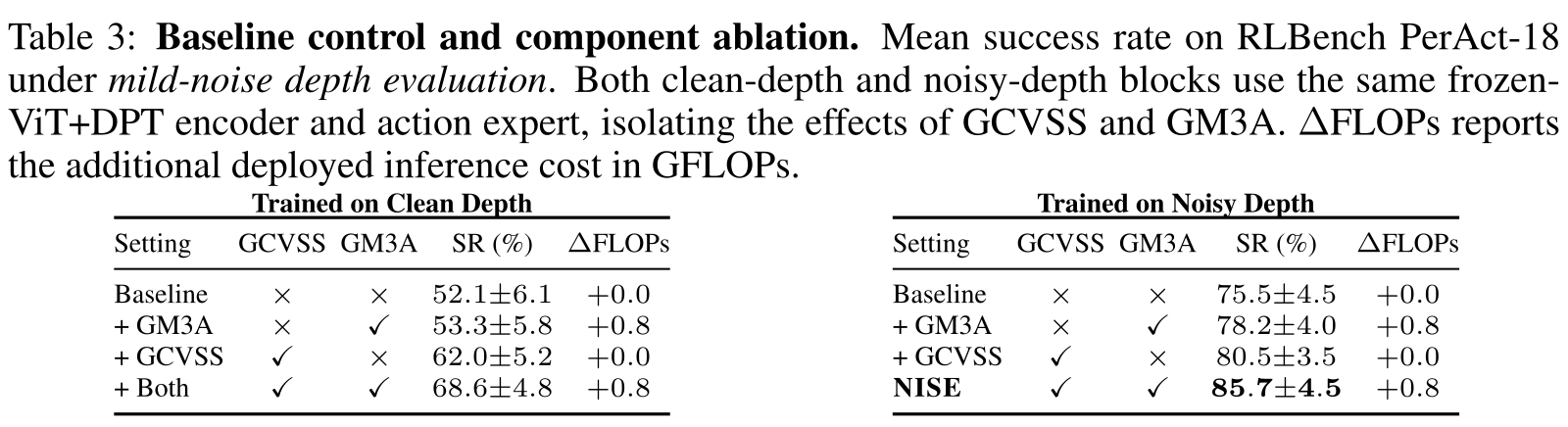
Complete original Table 3: Baseline control and component ablation. Mean success rate on RLBench PerAct-18 under mild-noise depth evaluation . Both clean-depth and noisy-depth blocks use the same frozen-ViT+DPT encoder and action expert, isolating the effects of GCVSS and GM3A. Δ \Delta FLOPs reports the additional deployed inference cost in GFLOPs.
Table 3: Baseline control and component ablation. Mean success rate on RLBench PerAct-18 under mild-noise depth evaluation. Both clean-depth and noisy-depth blocks use the same frozen-ViT+DPT encoder and action expert, isolating the effects of GCVSS and GM3A. Δ\DeltaFLOPs reports the additional deployed inference cost in GFLOPs.
Accessible table, original values and citation links
Trained on Clean Depth
Setting GCVSS GM3A SR (%) Δ\DeltaFLOPs
Baseline ×\times ×\times 52.1±6.152.1{\pm}6.1 +0.0+0.0
+ GM3A ×\times ✓\checkmark 53.3±5.853.3{\pm}5.8 +0.8+0.8
+ GCVSS ✓\checkmark ×\times 62.0±5.262.0{\pm}5.2 +0.0+0.0
+ Both ✓\checkmark ✓\checkmark 68.6±4.868.6{\pm}4.8 +0.8+0.8
Trained on Noisy Depth
Setting GCVSS GM3A SR (%) Δ\DeltaFLOPs
Baseline ×\times ×\times 75.5±4.575.5{\pm}4.5 +0.0+0.0
+ GM3A ×\times ✓\checkmark 78.2±4.078.2{\pm}4.0 +0.8+0.8
+ GCVSS ✓\checkmark ×\times 80.5±3.580.5{\pm}3.5 +0.0+0.0
NISE ✓\checkmark ✓\checkmark 85.7±4.5\mathbf{85.7{\pm}4.5} +0.8+0.8
Complete original Figure 4: Real-robot Success Rate. Each task group compares DP3, 3DDA, RVT-2, and NISE , with N = 30 N=30 trials per task and method.
Figure 4: Real-robot Success Rate. Each task group compares DP3, 3DDA, RVT-2, and NISE, with N=30N=30 trials per task and method.

5 Limitations and Conclusion

Cross-view supervision needs calibrated overlapping views and can reinforce shared wrong-background surfaces behind transparent objects. Local Gaussian attenuation only partially models biased/multimodal depth corruption. The paper supports improved empirical robustness on tested settings, with substantial real-task failures remaining. Its proposed future uncertainty models do not constitute completed solutions to those limits.

Acknowledgments

Support comes from Singapore’s National Robotics Programme 2.0 initiative on domain-specific robotics foundation models for manufacturing. The complete 42-reference bibliography remains.

Original paired RGB and depth demonstrations

The primary NISE project supplies six paired RGB/depth scenes: twelve unchanged original WebM clips with original source stills are retained here. They include transparent tube/lid observations and the five physical task demonstrations, with the repeated lid example deduplicated. RGB/depth views are labeled separately. The project’s interactive 3D diagnostics remain available through that link; selected clips are illustrations rather than additional quantitative trials.

Clean RGB of a bimanual scene with a mortar, pestle, and transparent test tube.
Raw depth of the same scene: missing measurements and distorted surfaces on the transparent test tube.
Close-up D405 wrist-camera RGB of a gripper removing the lid from a transparent petri dish.
Raw depth (D405 wrist) of the same petri-dish scene: the transparent dish and lid drop out into holes and unreliable surfaces.
Side-camera RGB of the single-arm gear-assembly demo.
Colorized sensor depth (Spectral_r) of the gear scene; reflective metal and edges drop into holes.
Side-camera RGB of the metal-pipe insertion demo.
Colorized sensor depth (Spectral_r); the reflective metal pipe and socket drop into holes.
Side-camera RGB of the bimanual pour-test-tube-into-mortar demo.
Colorized sensor depth (Spectral_r); the transparent test tube drops into holes and distorted surfaces.
D405 wrist RGB of the vision-sorted gear-collection demo (clear acrylic dividers).
Colorized sensor depth (Spectral_r); the clear acrylic surfaces drop into holes.

Appendix A Depth Corruption Model

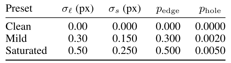
The full corruption model preserves all seven equations and preset values. Axial disparity noise grows approximately with depth squared; lateral jitter changes which surface is looked up; multiplicative masks introduce invalid values. Wrong-surface returns are produced by displaced lookup, not a separate independent Bernoulli variable. Mild/saturated presets use pixel jitter .30/.50, disparity standard deviation .150/.250, edge dropout .30/.50 and hole probability .002/.005. ‘Saturated’ is called ‘moderate’ in the implementation. The calibration protocol is described, but the manuscript does not enumerate every camera parameter, edge threshold or measured residual distribution needed to exactly reproduce calibration from text alone.

Equations 1–7
D~​(𝐮)=M⁡(𝐮)​[D⁡(𝐮)+ϵrange​(𝐮)+ϵedge​(𝐮)+ϵsurface​(𝐮)],\tilde{D}(\mathbf{u})=M(\mathbf{u})\left[D(\mathbf{u})+\epsilon_{\mathrm{range}}(\mathbf{u})+\epsilon_{\mathrm{edge}}(\mathbf{u})+\epsilon_{\mathrm{surface}}(\mathbf{u})\right], (1)
s⁡(𝐮)=f​bD⁡(𝐮),s~​(𝐮)=s⁡(𝐮)+ηs​(𝐮),Dax​(𝐮)=f​bs~​(𝐮),s(\mathbf{u})=\frac{fb}{D(\mathbf{u})},\qquad\tilde{s}(\mathbf{u})=s(\mathbf{u})+\eta_{s}(\mathbf{u}),\qquad D_{\mathrm{ax}}(\mathbf{u})=\frac{fb}{\tilde{s}(\mathbf{u})}, (2)
σz​(z)≈z2f​b​σs.\sigma_{z}(z)\approx\frac{z^{2}}{fb}\,\sigma_{s}. (3)
𝐮~=𝐮+𝜼ℓ,𝜼ℓ∼𝒩⁡(𝟎,σℓ2​I2).\tilde{\mathbf{u}}=\mathbf{u}+\boldsymbol{\eta}_{\ell},\qquad\boldsymbol{\eta}_{\ell}\sim\mathcal{N}(\mathbf{0},\sigma_{\ell}^{2}I_{2}). (4)
M⁡(𝐮)=Mvalid​(𝐮)​Medge​(𝐮)​Mhole​(𝐮),M(\mathbf{u})=M_{\mathrm{valid}}(\mathbf{u})\,M_{\mathrm{edge}}(\mathbf{u})\,M_{\mathrm{hole}}(\mathbf{u}), (5)
Medge(𝐮)∼Bernoulli(1−pedge 1{∥∇D(𝐮)∥>τ}),Mhole(𝐮)∼Bernoulli(1−phole).M_{\mathrm{edge}}(\mathbf{u})\sim\operatorname{Bernoulli}\!\left(1-p_{\mathrm{edge}}\,\mathbf{1}\{\|\nabla D(\mathbf{u})\|>\tau\}\right),\qquad M_{\mathrm{hole}}(\mathbf{u})\sim\operatorname{Bernoulli}(1-p_{\mathrm{hole}}). (6)
D~​(𝐮)=M⁡(𝐮)​Dax​(𝐮~),\tilde{D}(\mathbf{u})=M(\mathbf{u})\,D_{\mathrm{ax}}\!\left(\tilde{\mathbf{u}}\right), (7)
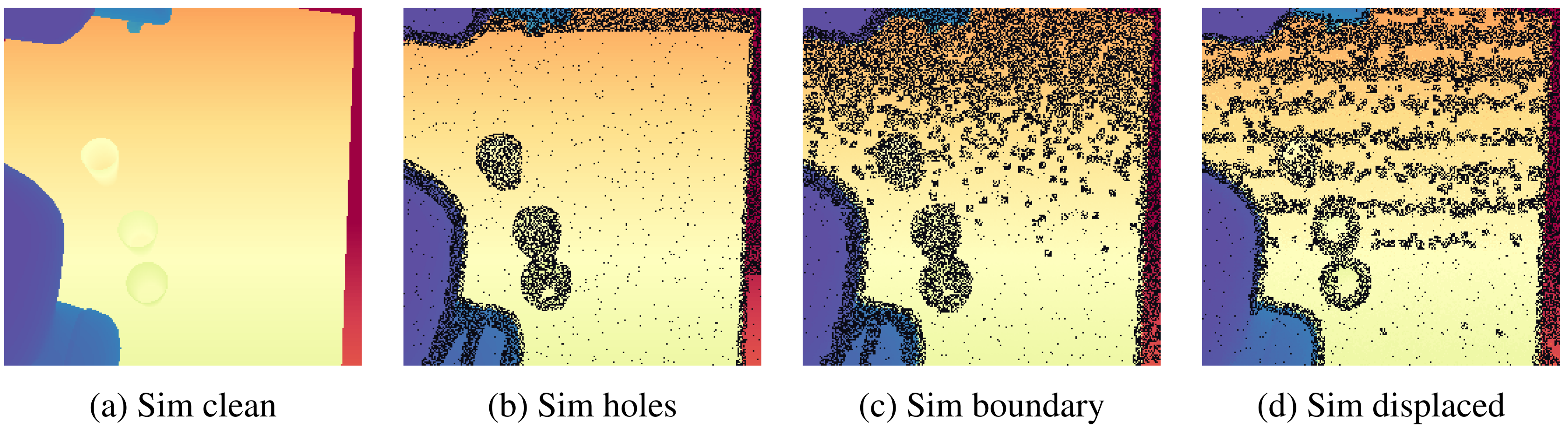
Complete original Figure 5: Depth-corruption families used as a controlled diagnostic. The panels show the simulator depth wrapper applied to a clean rendered frame, isolating random holes, boundary-localized artifacts, and displaced lookup near discontinuities.
The figure is a compact visual explanation of the procedural knobs in Equations 4 , 6 and 7 ; sensor-specific calibration is captured by the preset scales rather than by exact rendering of a single camera model.
Figure 5: Depth-corruption families used as a controlled diagnostic. The panels show the simulator depth wrapper applied to a clean rendered frame, isolating random holes, boundary-localized artifacts, and displaced lookup near discontinuities. The figure is a compact visual explanation of the procedural knobs in Equations 4, 6 and 7; sensor-specific calibration is captured by the preset scales rather than by exact rendering of a single camera model.
Complete original Table 4: Depth-noise presets. The main paper uses clean, mild, and saturated; saturated corresponds to the high-stress endpoint used in the teaser and main summary table.
Saturated is named moderate in the implementation, with the same parameter values.
Table 4: Depth-noise presets. The main paper uses clean, mild, and saturated; saturated corresponds to the high-stress endpoint used in the teaser and main summary table. Saturated is named moderate in the implementation, with the same parameter values.
Accessible table, original values and citation links
Preset σℓ\sigma_{\ell} (px) σs\sigma_{s} (px) pedgep_{\mathrm{edge}} pholep_{\mathrm{hole}}
Clean 0.00 0.000 0.000 0.0000
Mild 0.30 0.150 0.300 0.0020
Saturated 0.50 0.250 0.500 0.0050

Appendix B Visual Backbone and Policy Ablations

Backbone controls separate a strong pretrained spatial representation from the proposed learning/attention changes. Their absolute scores use distinct evaluation/noise protocols, so native-stack and full-stack numbers should not be pooled as one benchmark row.

B.1 Visual Backbone

The public VGGT-Omega checkpoint is frozen. A trainable DPT aggregator and DDPM action expert consume its features. This large geometry-pretrained base is shared by the same-stack controls.

B.2 Same-Stack Base-Model Control

Under clean-input evaluation with the same stack/training recipe, disabling both mechanisms gives 79.0±5.0%, while NISE gives 89.0±4.3%. This is the reported within-stack clean-input benefit. It complements, rather than replaces, the mild-noise component comparison and published-baseline table.

B.3 Native-Policy Ablations on 3DDA and RVT-2

Three-task native 3DDA and RVT-2 controls retain each architecture and fine-tune all variants on saturated-noise demonstrations. Combined modules raise saturated means 56.7→70.3% and 24.0→44.0%, respectively. 3DDA’s higher noisy than clean score reflects specialization to that training distribution. These are three-task means, not the full eighteen-task Table 2 protocol.
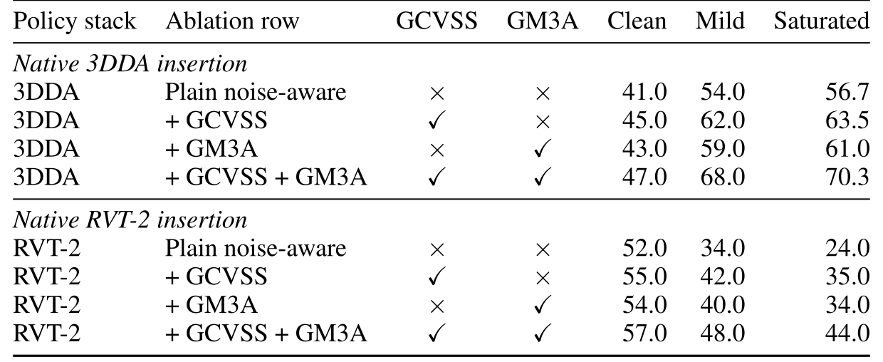
Complete original Table 5: Native-stack ablations on RLBench. Success rates (%) are means over three RLBench tasks: push_buttons, insert_peg, and stack_cups.
The 3DDA block keeps the native 3DDA feature pyramid and diffusion action expert; the RVT-2 block keeps the virtual-view/keypose policy family.
Within each policy block, all four variants are fine-tuned on saturated-noise demonstrations using the same protocol, varying only the inclusion of GCVSS and GM3A.
Table 5: Native-stack ablations on RLBench. Success rates (%) are means over three RLBench tasks: push_buttons, insert_peg, and stack_cups. The 3DDA block keeps the native 3DDA feature pyramid and diffusion action expert; the RVT-2 block keeps the virtual-view/keypose policy family. Within each policy block, all four variants are fine-tuned on saturated-noise demonstrations using the same protocol, varying only the inclusion of GCVSS and GM3A.
Accessible table, original values and citation links
Policy stack Ablation row GCVSS GM3A Clean Mild Saturated
Native 3DDA insertion
3DDA Plain noise-aware ×\times ×\times 41.0 54.0 56.7
3DDA + GCVSS ✓\checkmark ×\times 45.0 62.0 63.5
3DDA + GM3A ×\times ✓\checkmark 43.0 59.0 61.0
3DDA + GCVSS + GM3A ✓\checkmark ✓\checkmark 47.0 68.0 70.3
Native RVT-2 insertion
RVT-2 Plain noise-aware ×\times ×\times 52.0 34.0 24.0
RVT-2 + GCVSS ✓\checkmark ×\times 55.0 42.0 35.0
RVT-2 + GM3A ×\times ✓\checkmark 54.0 40.0 34.0
RVT-2 + GCVSS + GM3A ✓\checkmark ✓\checkmark 57.0 48.0 44.0

Appendix C Depth-Repair Front-End Comparisons

Adding D3RoMa or Marigold-DC repair raises saturated NISE mean 84.1→84.8/85.2%, with similar clean scores. The changes are modest relative to the listed deviations; no significance test is supplied. Main results use raw depth. Repair and representation learning can be complementary without repair being required for NISE inference.

Complete original Table 6: Effect of depth repair on NISE . Mean success rate ± \pm standard deviation (%) on RLBench PerAct-18 under clean, mild-noise, and saturated-noise evaluation.
We compare NISE with raw depth and with depth preprocessed by D3RoMa or Marigold-DC before the policy consumes RGB-D.
Best means per column are bold.
Table 6: Effect of depth repair on NISE. Mean success rate ±\pm standard deviation (%) on RLBench PerAct-18 under clean, mild-noise, and saturated-noise evaluation. We compare NISE with raw depth and with depth preprocessed by D3RoMa or Marigold-DC before the policy consumes RGB-D. Best means per column are bold.
Accessible table, original values and citation links
Input / policy Clean Mild Saturated
NISE + raw depth 89.0±4.389.0{\pm}4.3 85.7±4.585.7{\pm}4.5 84.1±4.684.1{\pm}4.6
NISE + D3RoMa repair 89.0±4.289.0{\pm}4.2 86.1±4.386.1{\pm}4.3 84.8±4.584.8{\pm}4.5
NISE + Marigold-DC repair 89.1±4.1\mathbf{89.1{\pm}4.1} 86.4±4.2\mathbf{86.4{\pm}4.2} 85.2±4.4\mathbf{85.2{\pm}4.4}

C.1 CDM and NISE on Real-Robot

On thirty lid-removal trials per configuration, same-stack baseline gives 15/30 raw and 18/30 CDM; NISE gives 20/30 raw and 23/30 CDM. Repair adds three successes in both policies, while NISE adds five with either depth source. This is a controlled single-task complementarity result, rather than a general additive law across all materials/tasks.
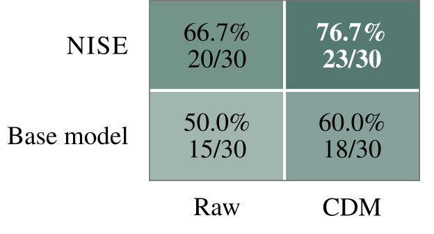
Complete original Figure 6: CDM × \times policy control on real-robot lid removal. Evaluation uses Remove the Petri Lid under real sensor noise, with 30 30 trials per configuration.
Each cell reports the success rate and successful trials out of 30 30 .
The base model uses the same policy stack as NISE with GCVSS and GM3A disabled.
Figure 6: CDM ×\times policy control on real-robot lid removal. Evaluation uses Remove the Petri Lid under real sensor noise, with 3030 trials per configuration. Each cell reports the success rate and successful trials out of 3030. The base model uses the same policy stack as NISE with GCVSS and GM3A disabled.

Appendix D GCVSS Target-Construction Ablation

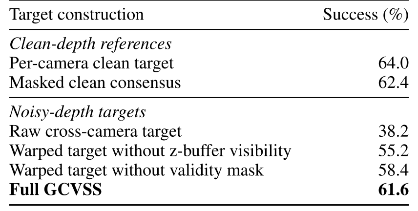
On saturated Stack Cups, raw cross-camera supervision scores 38.2%; full calibrated/filtered GCVSS reaches 61.6%, near clean-target references 64.0/62.4%. Removing z-buffer visibility or validity masking gives 55.2/58.4%. Depth correlation rises .14→.367 and logged gradient cosine −.050→+.027. Those small cosine values indicate weak alignment, not strong proof of identical optimization signals. The complete three-panel warp/mask diagnostic remains.
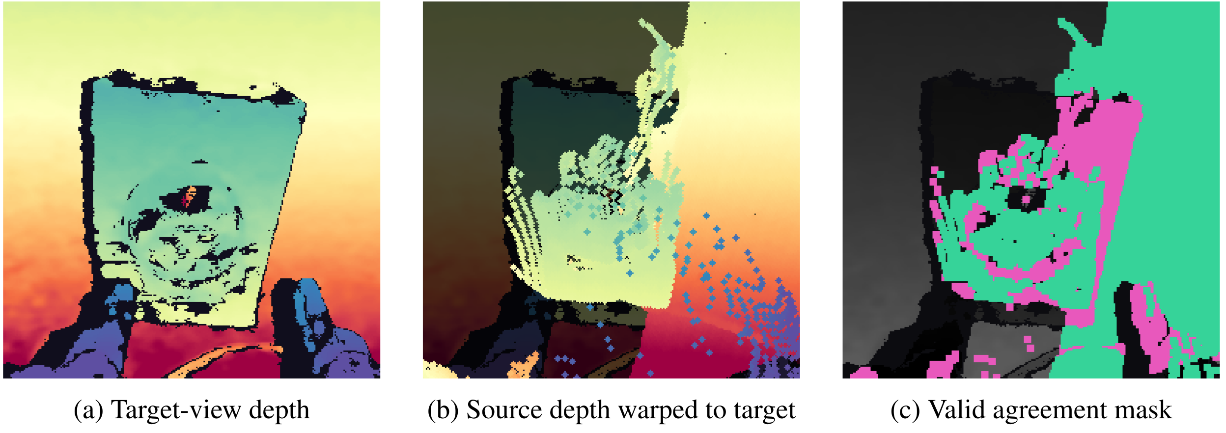
Complete original Figure 7: Cross-view depth becomes a geometry target only after calibrated warping. The source camera is forward-warped into the target camera frame and filtered by a visibility/validity mask before it supervises the shared feature map.
This is the practical difference between a raw cross-camera noisy target and GCVSS: the auxiliary signal is still noisy, but it is expressed in the same camera frame as the target feature map.
Figure 7: Cross-view depth becomes a geometry target only after calibrated warping. The source camera is forward-warped into the target camera frame and filtered by a visibility/validity mask before it supervises the shared feature map. This is the practical difference between a raw cross-camera noisy target and GCVSS: the auxiliary signal is still noisy, but it is expressed in the same camera frame as the target feature map.
Complete original Table 7: GCVSS target-construction and component ablation. Success rates (%) on RLBench Stack Cups under saturated depth corruption.
All variants use the same policy stack and training budget.
The component controls remove z-buffer visibility filtering or validity masking from the full calibrated cross-view target construction.
Clean-depth targets are simulation references; the best noisy-depth variant is bold.
Table 7: GCVSS target-construction and component ablation. Success rates (%) on RLBench Stack Cups under saturated depth corruption. All variants use the same policy stack and training budget. The component controls remove z-buffer visibility filtering or validity masking from the full calibrated cross-view target construction. Clean-depth targets are simulation references; the best noisy-depth variant is bold.
Accessible table, original values and citation links
Target construction Success (%)
Clean-depth references
Per-camera clean target 64.0
Masked clean consensus 62.4
Noisy-depth targets
Raw cross-camera target 38.2
Warped target without z-buffer visibility 55.2
Warped target without validity mask 58.4
Full GCVSS 61.6

D.1 Multi-View Agreement on Transparent Objects

Visibility agreement is not ground-truth correctness. Cameras looking through transparent material can agree on the background rather than the hidden object surface. RGB context and adaptive attention remain available but do not guarantee recovering that geometry.

Appendix E GM3A Ablations

The appendix separates fixed frequency attenuation from adaptive residuals, then holds GCVSS fixed to compare task sensitivity. The learned coefficients are anchored to a Gaussian prior through the policy objective.

E.1 Frequency-Only versus Adaptive Attenuation

On three tasks, adaptive attenuation gives 85.3/77.3/73.3% for clean/mild/saturated depth, versus 79.3/70.7/66.7% with a token-independent σ=1 frequency profile. This comparison changes both adaptation and its relationship to the sensor prior, so it is evidence for this adaptive design rather than an isolated proof that all fixed profiles are inferior.
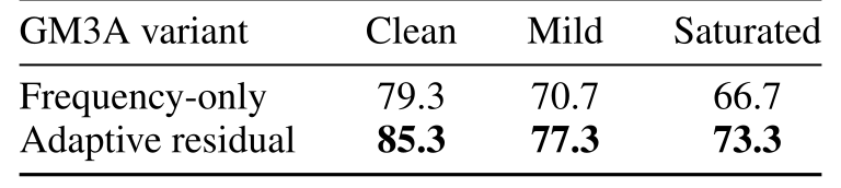
Complete original Table 8: Frequency-only versus adaptive GM3A. Success rates (%) across three RLBench tasks (Push Buttons, Insert Peg, and Stack Cups) under clean, mild-noise, and saturated-noise evaluation.
Both variants use the same training data and seeds.
Table 8: Frequency-only versus adaptive GM3A. Success rates (%) across three RLBench tasks (Push Buttons, Insert Peg, and Stack Cups) under clean, mild-noise, and saturated-noise evaluation. Both variants use the same training data and seeds.
Accessible table, original values and citation links
GM3A variant Clean Mild Saturated
Frequency-only 79.3 70.7 66.7
Adaptive residual 85.3 77.3 73.3

E.2 Precision-Task GM3A Analysis

With GCVSS fixed, GM3A leaves push-buttons/open-drawer/turn-tap means unchanged and raises insertion/stacking means by ten points under mild noise. The tested precision-sensitive tasks benefit more. These five cases do not establish a universal taxonomy of which tasks need each frequency band.
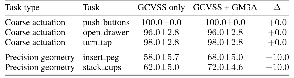
Complete original Table 9: Precision-task GM3A analysis. Success rates (%) are measured on five RLBench tasks under mild-noise evaluation with the same-stack noisy-depth policy.
The comparison fixes GCVSS and toggles GM3A, isolating the deployed attention change.
GM3A yields larger gains on the tested precision-sensitive tasks, while coarse-task means are unchanged.
Table 9: Precision-task GM3A analysis. Success rates (%) are measured on five RLBench tasks under mild-noise evaluation with the same-stack noisy-depth policy. The comparison fixes GCVSS and toggles GM3A, isolating the deployed attention change. GM3A yields larger gains on the tested precision-sensitive tasks, while coarse-task means are unchanged.
Accessible table, original values and citation links
Task type Task GCVSS only GCVSS + GM3A Δ\Delta
Coarse actuation push_buttons 100.0±0.0100.0{\pm}0.0 100.0±0.0100.0{\pm}0.0 +0.0+0.0
Coarse actuation open_drawer 96.0±2.896.0{\pm}2.8 96.0±2.896.0{\pm}2.8 +0.0+0.0
Coarse actuation turn_tap 98.0±2.898.0{\pm}2.8 98.0±2.898.0{\pm}2.8 +0.0+0.0
Precision geometry insert_peg 58.0±5.758.0{\pm}5.7 68.0±5.068.0{\pm}5.0 +10.0+10.0
Precision geometry stack_cups 62.0±5.062.0{\pm}5.0 72.0±4.672.0{\pm}4.6 +10.0+10.0

Appendix F Feature-Invariance and Dampening Diagnostics

Same-scene tests vary only depth while holding RGB, proprioception, calibration and action labels fixed. NISE lowers mild/saturated cosine drift to .12/.17 and raises CKA to .89/.84, compared with .31/.48 and .68/.54 for the noisy-trained same-stack baseline. Region diagnostics show stronger high-frequency suppression at depth boundaries, transparent/specular proxies and precision contacts. Contact masks use ground-truth interaction neighborhoods for analysis; they are not additional deployed sensors. ‘Invariant’ here means reduced measured sensitivity.

Complete original Table 10: Direct feature-stability diagnostic on RLBench. Same-scene paired evaluation compares the shared feature map under clean depth against the same RGB/proprioception with mild or saturated corrupted depth.
Cosine drift is lower-is-better; CKA is higher-is-better.
The mild-noise SR column reports the corresponding same-stack success rate when available.
Table 10: Direct feature-stability diagnostic on RLBench. Same-scene paired evaluation compares the shared feature map under clean depth against the same RGB/proprioception with mild or saturated corrupted depth. Cosine drift is lower-is-better; CKA is higher-is-better. The mild-noise SR column reports the corresponding same-stack success rate when available.
Accessible table, original values and citation links
Setting Mild drift ↓\downarrow Mild CKA ↑\uparrow Saturated drift ↓\downarrow Saturated CKA ↑\uparrow Mild SR (%)
Clean-trained same-stack baseline 0.44 0.55 0.63 0.39 52.1
Noisy-trained same-stack baseline 0.31 0.68 0.48 0.54 75.5
+ GM3A 0.28 0.71 0.42 0.59 78.2
+ GCVSS 0.18 0.82 0.26 0.74 80.5
NISE 0.12 0.89 0.17 0.84 85.7
Complete original Table 11: GM3A dampening by task and region. Values report mean high-frequency dampening 1 − α 1-\alpha on saturated-depth RLBench and real-robot diagnostic frames; larger values indicate stronger suppression of unreliable 3D positional phase.
GM3A keeps reliable regions close to ordinary 3D-RoPE while increasing dampening around depth boundaries, transparent/specular proxies, and precision-task contact regions.
Table 11: GM3A dampening by task and region. Values report mean high-frequency dampening 1−α1-\alpha on saturated-depth RLBench and real-robot diagnostic frames; larger values indicate stronger suppression of unreliable 3D positional phase. GM3A keeps reliable regions close to ordinary 3D-RoPE while increasing dampening around depth boundaries, transparent/specular proxies, and precision-task contact regions.
Accessible table, original values and citation links
Task type Task Reliable surface Depth boundary Transparent/specular proxy Contact region
Coarse push_buttons 0.06 0.15 0.18 0.10
Coarse open_drawer 0.07 0.16 0.19 0.12
Precision insert_peg 0.08 0.27 0.31 0.29
Precision stack_cups 0.09 0.25 0.34 0.28
Real transparent remove_petri_lid 0.10 0.31 0.39 0.32
Real transparent pour_test_tube 0.11 0.33 0.42 0.35

Appendix G Training, Implementation, and Runtime

Training and runtime details distinguish frozen, trainable, training-only and deployed components. Inference overhead is measured against the same large base model, with rendering and robot I/O excluded.

G.1 Training Configuration

Training uses 32-bit LAMB, cosine decay, 300k updates and global batch 64, with head/policy learning rates 5e-5/1e-4. The DPT head fuses ViT layers 4/11/17/23, projects 2048→120 channels and has 2.283M trainable parameters. Geometry decoding is 120→64→32→16→1; views pair round-robin [1,2,3,0]. Two GM3A MLPs each map XYZ+range through 4→64→60. RLBench geometry targets are cross-view; single-view MetaWorld targets are clean simulator depth. Real baselines share data but retain their tuned training recipes.

G.2 Clean-Only and Mixed-Noise Training on RLBench

Mixed-noise NISE gives 89.0/85.7/84.1%, versus clean-only NISE 89.7/68.6/63.0%. Clean-only 3DDA gives 81.3/55.0/15.0%. Noise exposure remains a major part of robustness; the architecture alone does not remove the need for varied training reliability. One trained policy serves all three evaluation levels.
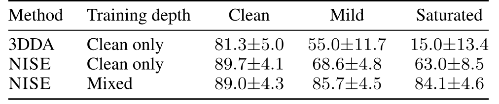
Complete original Table 12: Clean-only and mixed-noise training on RLBench PerAct-18. Task-averaged success rates (%, mean ± \pm standard deviation) on RLBench PerAct-18 under clean, mild, and saturated depth evaluation.
Clean-only training uses clean simulator depth; mixed training samples clean/mild/saturated inputs with a 1 : 1 : 1 1{:}1{:}1 ratio.
The mixed-training NISE row reproduces Table 2 , with ± \pm denoting the standard deviation across three independent training runs.
Table 12: Clean-only and mixed-noise training on RLBench PerAct-18. Task-averaged success rates (%, mean ±\pm standard deviation) on RLBench PerAct-18 under clean, mild, and saturated depth evaluation. Clean-only training uses clean simulator depth; mixed training samples clean/mild/saturated inputs with a 1:1:11{:}1{:}1 ratio. The mixed-training NISE row reproduces Table 2, with ±\pm denoting the standard deviation across three independent training runs.
Accessible table, original values and citation links
Method Training depth Clean Mild Saturated
3DDA Clean only 81.3±5.081.3{\pm}5.0 55.0±11.755.0{\pm}11.7 15.0±13.415.0{\pm}13.4
NISE Clean only 89.7±4.189.7{\pm}4.1 68.6±4.868.6{\pm}4.8 63.0±8.563.0{\pm}8.5
NISE Mixed 89.0±4.389.0{\pm}4.3 85.7±4.585.7{\pm}4.5 84.1±4.684.1{\pm}4.6

G.3 Implementation and Runtime Cost

The deployed policy has 912.68M total parameters, mostly a 907.92M frozen backbone; 4.76M belong to trainable modules by the stated counting convention. GM3A adds 8440 deployed parameters and .8 GFLOPs; the 164321-parameter geometry head is training-only. RTX 5080 four-view batch-one policy forward time is 37.5±.6 ms versus baseline 36.1±.4, about 26.6 versus 27.7 Hz. This excludes rendering/I/O and precomputed instruction encoding, so it is not a full robot control-loop rate.

Complete original Table 13: Runtime and deployed parameter and FLOP overhead. Measurements use the RLBench PerAct-18 same-stack policy with four RGB-D views, batch size one, and policy-forward timing on the RTX 5080 after warmup.
Timing excludes simulator rendering and robot I/O. Δ \Delta Params (thousands) and Δ \Delta FLOPs (GFLOPs) report deployed overhead relative to the same-stack baseline without GCVSS or GM3A; the training-only GCVSS head is excluded.
Table 13: Runtime and deployed parameter and FLOP overhead. Measurements use the RLBench PerAct-18 same-stack policy with four RGB-D views, batch size one, and policy-forward timing on the RTX 5080 after warmup. Timing excludes simulator rendering and robot I/O. Δ\DeltaParams (thousands) and Δ\DeltaFLOPs (GFLOPs) report deployed overhead relative to the same-stack baseline without GCVSS or GM3A; the training-only GCVSS head is excluded.
Accessible table, original values and citation links
Setting GCVSS GM3A Δ\DeltaParams (K) Δ\DeltaFLOPs Latency (ms) Throughput (Hz)
Same-stack baseline ×\times ×\times 00 +0.0+0.0 36.1±0.436.1{\pm}0.4 27.727.7
+ GCVSS ✓\checkmark ×\times 00 +0.0+0.0 36.2±0.536.2{\pm}0.5 27.627.6
+ GM3A ×\times ✓\checkmark 8.448.44 +0.8+0.8 37.4±0.537.4{\pm}0.5 26.726.7
NISE ✓\checkmark ✓\checkmark 8.448.44 +0.8+0.8 37.5±0.637.5{\pm}0.6 26.626.6

Appendix H MetaWorld Per-Task Results

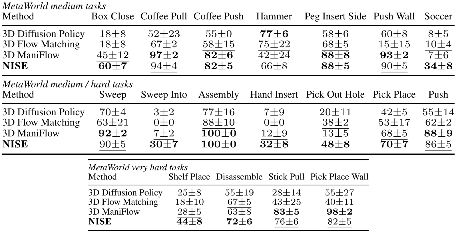
The complete clean-depth tables report 46 named MetaWorld tasks in seven panels; their NISE means average exactly 79.0%. Deviations here are repeated-evaluation variation, distinct from Table 2’s three-training-run variability. NISE is not best on every task: strong baselines retain advantages on several easy tasks and difficult stick/wall variants. All task names, ties and emphasis remain with their own protocols.
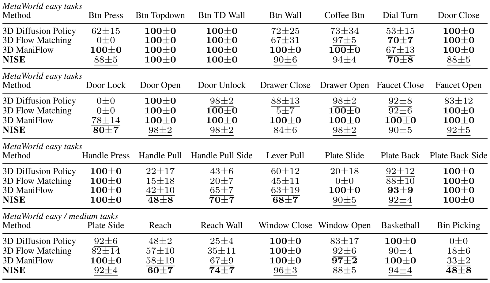
Complete original Table 14: MetaWorld per-task results, part I. The NISE row reports clean-depth success rates from our MetaWorld protocol.
Values are success rates (%).
For NISE , ± \pm denotes the standard deviation across repeated evaluations.
The best and second-best distinct means per column are bold and underlined, respectively, including ties.
Table 14: MetaWorld per-task results, part I. The NISE row reports clean-depth success rates from our MetaWorld protocol. Values are success rates (%). For NISE, ±\pm denotes the standard deviation across repeated evaluations. The best and second-best distinct means per column are bold and underlined, respectively, including ties.
Accessible table, original values and citation links
MetaWorld easy tasks
Method Btn Press Btn Topdown Btn TD Wall Btn Wall Coffee Btn Dial Turn Door Close
3D Diffusion Policy 62±1562{\pm}15 𝟏𝟎𝟎±𝟎\mathbf{100{\pm}0} 𝟏𝟎𝟎±𝟎\mathbf{100{\pm}0} 72±2572{\pm}25 73±3473{\pm}34 53±1553{\pm}15 𝟏𝟎𝟎±𝟎\mathbf{100{\pm}0}
3D Flow Matching 0±00{\pm}0 𝟏𝟎𝟎±𝟎\mathbf{100{\pm}0} 𝟏𝟎𝟎±𝟎\mathbf{100{\pm}0} 67±3167{\pm}31 97±5¯\underline{97{\pm}5} 𝟕𝟎±𝟕\mathbf{70{\pm}7} 𝟏𝟎𝟎±𝟎\mathbf{100{\pm}0}
3D ManiFlow 𝟏𝟎𝟎±𝟎\mathbf{100{\pm}0} 𝟏𝟎𝟎±𝟎\mathbf{100{\pm}0} 𝟏𝟎𝟎±𝟎\mathbf{100{\pm}0} 𝟏𝟎𝟎±𝟎\mathbf{100{\pm}0} 𝟏𝟎𝟎±𝟎\mathbf{100{\pm}0} 67±13¯\underline{67{\pm}13} 𝟏𝟎𝟎±𝟎\mathbf{100{\pm}0}
NISE 88±5¯\underline{88{\pm}5} 𝟏𝟎𝟎±𝟎\mathbf{100{\pm}0} 𝟏𝟎𝟎±𝟎\mathbf{100{\pm}0} 90±6¯\underline{90{\pm}6} 94±494{\pm}4 𝟕𝟎±𝟖\mathbf{70{\pm}8} 88±5¯\underline{88{\pm}5}
MetaWorld easy tasks
Method Door Lock Door Open Door Unlock Drawer Close Drawer Open Faucet Close Faucet Open
3D Diffusion Policy 0±00{\pm}0 𝟏𝟎𝟎±𝟎\mathbf{100{\pm}0} 98±2¯\underline{98{\pm}2} 88±13¯\underline{88{\pm}13} 98±2¯\underline{98{\pm}2} 92±8¯\underline{92{\pm}8} 83±1283{\pm}12
3D Flow Matching 0±00{\pm}0 𝟏𝟎𝟎±𝟎\mathbf{100{\pm}0} 𝟏𝟎𝟎±𝟎\mathbf{100{\pm}0} 5±75{\pm}7 𝟏𝟎𝟎±𝟎\mathbf{100{\pm}0} 92±6¯\underline{92{\pm}6} 𝟏𝟎𝟎±𝟎\mathbf{100{\pm}0}
3D ManiFlow 78±14¯\underline{78{\pm}14} 𝟏𝟎𝟎±𝟎\mathbf{100{\pm}0} 𝟏𝟎𝟎±𝟎\mathbf{100{\pm}0} 𝟏𝟎𝟎±𝟎\mathbf{100{\pm}0} 𝟏𝟎𝟎±𝟎\mathbf{100{\pm}0} 𝟏𝟎𝟎±𝟎\mathbf{100{\pm}0} 𝟏𝟎𝟎±𝟎\mathbf{100{\pm}0}
NISE 𝟖𝟎±𝟕\mathbf{80{\pm}7} 98±2¯\underline{98{\pm}2} 98±2¯\underline{98{\pm}2} 84±684{\pm}6 98±2¯\underline{98{\pm}2} 90±590{\pm}5 92±5¯\underline{92{\pm}5}
MetaWorld easy tasks
Method Handle Press Handle Pull Handle Pull Side Lever Pull Plate Slide Plate Back Plate Back Side
3D Diffusion Policy 𝟏𝟎𝟎±𝟎\mathbf{100{\pm}0} 22±1722{\pm}17 43±643{\pm}6 60±1260{\pm}12 20±1820{\pm}18 92±12¯\underline{92{\pm}12} 𝟏𝟎𝟎±𝟎\mathbf{100{\pm}0}
3D Flow Matching 𝟏𝟎𝟎±𝟎\mathbf{100{\pm}0} 15±1815{\pm}18 20±720{\pm}7 45±1145{\pm}11 0±00{\pm}0 88±1088{\pm}10 𝟏𝟎𝟎±𝟎\mathbf{100{\pm}0}
3D ManiFlow 𝟏𝟎𝟎±𝟎\mathbf{100{\pm}0} 42±10¯\underline{42{\pm}10} 65±7¯\underline{65{\pm}7} 63±19¯\underline{63{\pm}19} 𝟏𝟎𝟎±𝟎\mathbf{100{\pm}0} 𝟗𝟑±𝟗\mathbf{93{\pm}9} 𝟏𝟎𝟎±𝟎\mathbf{100{\pm}0}
NISE 𝟏𝟎𝟎±𝟎\mathbf{100{\pm}0} 𝟒𝟖±𝟖\mathbf{48{\pm}8} 𝟕𝟎±𝟕\mathbf{70{\pm}7} 𝟔𝟖±𝟕\mathbf{68{\pm}7} 90±5¯\underline{90{\pm}5} 92±4¯\underline{92{\pm}4} 𝟏𝟎𝟎±𝟎\mathbf{100{\pm}0}
MetaWorld easy / medium tasks
Method Plate Side Reach Reach Wall Window Close Window Open Basketball Bin Picking
3D Diffusion Policy 92±6¯\underline{92{\pm}6} 48±248{\pm}2 25±425{\pm}4 𝟏𝟎𝟎±𝟎\mathbf{100{\pm}0} 83±1783{\pm}17 𝟏𝟎𝟎±𝟎\mathbf{100{\pm}0} 0±00{\pm}0
3D Flow Matching 82±1482{\pm}14 57±1057{\pm}10 35±1135{\pm}11 𝟏𝟎𝟎±𝟎\mathbf{100{\pm}0} 92±6¯\underline{92{\pm}6} 90±490{\pm}4 18±618{\pm}6
3D ManiFlow 𝟏𝟎𝟎±𝟎\mathbf{100{\pm}0} 58±19¯\underline{58{\pm}19} 67±9¯\underline{67{\pm}9} 𝟏𝟎𝟎±𝟎\mathbf{100{\pm}0} 𝟗𝟕±𝟐\mathbf{97{\pm}2} 𝟏𝟎𝟎±𝟎\mathbf{100{\pm}0} 33±2¯\underline{33{\pm}2}
NISE 92±4¯\underline{92{\pm}4} 𝟔𝟎±𝟕\mathbf{60{\pm}7} 𝟕𝟒±𝟕\mathbf{74{\pm}7} 96±3¯\underline{96{\pm}3} 88±588{\pm}5 94±4¯\underline{94{\pm}4} 𝟒𝟖±𝟖\mathbf{48{\pm}8}
Complete original Table 15: MetaWorld per-task results, part II. This table continues the clean-depth per-task comparison in Table 14 .
The best and second-best distinct means per column are bold and underlined, respectively, including ties.
Table 15: MetaWorld per-task results, part II. This table continues the clean-depth per-task comparison in Table 14. The best and second-best distinct means per column are bold and underlined, respectively, including ties.
Accessible table, original values and citation links
MetaWorld medium tasks
Method Box Close Coffee Pull Coffee Push Hammer Peg Insert Side Push Wall Soccer
3D Diffusion Policy 18±818{\pm}8 52±2352{\pm}23 55±055{\pm}0 𝟕𝟕±𝟔\mathbf{77{\pm}6} 58±658{\pm}6 60±860{\pm}8 8±58{\pm}5
3D Flow Matching 18±818{\pm}8 67±267{\pm}2 58±15¯\underline{58{\pm}15} 75±22¯\underline{75{\pm}22} 68±5¯\underline{68{\pm}5} 15±1515{\pm}15 10±4¯\underline{10{\pm}4}
3D ManiFlow 45±12¯\underline{45{\pm}12} 𝟗𝟕±𝟐\mathbf{97{\pm}2} 𝟖𝟐±𝟔\mathbf{82{\pm}6} 42±2442{\pm}24 𝟖𝟖±𝟖\mathbf{88{\pm}8} 𝟗𝟑±𝟐\mathbf{93{\pm}2} 7±67{\pm}6
NISE 𝟔𝟎±𝟕\mathbf{60{\pm}7} 94±4¯\underline{94{\pm}4} 𝟖𝟐±𝟓\mathbf{82{\pm}5} 66±866{\pm}8 𝟖𝟖±𝟓\mathbf{88{\pm}5} 90±5¯\underline{90{\pm}5} 𝟑𝟒±𝟖\mathbf{34{\pm}8}
MetaWorld medium / hard tasks
Method Sweep Sweep Into Assembly Hand Insert Pick Out Hole Pick Place Push
3D Diffusion Policy 70±470{\pm}4 3±23{\pm}2 77±1677{\pm}16 7±97{\pm}9 20±1120{\pm}11 42±542{\pm}5 55±1455{\pm}14
3D Flow Matching 63±2163{\pm}21 0±00{\pm}0 88±10¯\underline{88{\pm}10} 0±00{\pm}0 38±2¯\underline{38{\pm}2} 53±1753{\pm}17 62±262{\pm}2
3D ManiFlow 𝟗𝟐±𝟐\mathbf{92{\pm}2} 7±2¯\underline{7{\pm}2} 𝟏𝟎𝟎±𝟎\mathbf{100{\pm}0} 12±9¯\underline{12{\pm}9} 13±513{\pm}5 68±5¯\underline{68{\pm}5} 𝟖𝟖±𝟗\mathbf{88{\pm}9}
NISE 90±5¯\underline{90{\pm}5} 𝟑𝟎±𝟕\mathbf{30{\pm}7} 𝟏𝟎𝟎±𝟎\mathbf{100{\pm}0} 𝟑𝟐±𝟖\mathbf{32{\pm}8} 𝟒𝟖±𝟖\mathbf{48{\pm}8} 𝟕𝟎±𝟕\mathbf{70{\pm}7} 86±5¯\underline{86{\pm}5}
MetaWorld very hard tasks
Method Shelf Place Disassemble Stick Pull Pick Place Wall
3D Diffusion Policy 25±825{\pm}8 55±1955{\pm}19 28±1428{\pm}14 55±2755{\pm}27
3D Flow Matching 18±1018{\pm}10 67±5¯\underline{67{\pm}5} 43±2543{\pm}25 40±1140{\pm}11
3D ManiFlow 28±5¯\underline{28{\pm}5} 63±863{\pm}8 𝟖𝟑±𝟓\mathbf{83{\pm}5} 𝟗𝟖±𝟐\mathbf{98{\pm}2}
NISE 𝟒𝟒±𝟖\mathbf{44{\pm}8} 𝟕𝟐±𝟔\mathbf{72{\pm}6} 76±6¯\underline{76{\pm}6} 82±5¯\underline{82{\pm}5}

Appendix I Real-Robot Protocol and Confidence Intervals

Each of five real tasks has thirty rollouts per method, varied placements and manual resets. Binary terminal/video criteria are explicitly task-specific; tube success is a grasp moved over the mortar into the pouring pose. Table 16 retains all twenty counts and Wilson 95% intervals from the exact formula. The small binomial samples quantify substantial uncertainty and are not independent training-seed or cross-site studies. The manuscript does not supply full demonstration counts or a detailed placement distribution.

Equation 8
p^W=p^+z2/(2​n)1+z2/n,hW=z1+z2/n​p^​(1−p^)n+z24​n2.\hat{p}_{\mathrm{W}}=\frac{\hat{p}+z^{2}/(2n)}{1+z^{2}/n},\qquad h_{\mathrm{W}}=\frac{z}{1+z^{2}/n}\sqrt{\frac{\hat{p}(1-\hat{p})}{n}+\frac{z^{2}}{4n^{2}}}. (8)
Complete original Table 16: Real-robot per-task trial counts with Wilson 95% confidence intervals. Each task entry is k / 30 k/30 successes, success rate (%), and Wilson interval.
Table 16: Real-robot per-task trial counts with Wilson 95% confidence intervals. Each task entry is k/30k/30 successes, success rate (%), and Wilson interval.
Accessible table, original values and citation links
Task DP3 3DDA RVT-2 NISE
Assemble the Gear 4/30, 13.3 [5.3, 29.7] 7/30, 23.3 [11.8, 40.9] 11/30, 36.7 [21.9, 54.5] 25/30, 83.3 [66.4, 92.7]
Remove the Petri Lid 6/30, 20.0 [9.5, 37.3] 10/30, 33.3 [19.2, 51.2] 5/30, 16.7 [7.3, 33.6] 20/30, 66.7 [48.8, 80.8]
Insert the Metal Pipe 3/30, 10.0 [3.5, 25.6] 8/30, 26.7 [14.2, 44.4] 12/30, 40.0 [24.6, 57.7] 22/30, 73.3 [55.6, 85.8]
Pour Test Tube into Mortar 2/30, 6.7 [1.8, 21.3] 6/30, 20.0 [9.5, 37.3] 4/30, 13.3 [5.3, 29.7] 13/30, 43.3 [27.4, 60.8]
Vision-Sorted Gear Collection 4/30, 13.3 [5.3, 29.7] 3/30, 10.0 [3.5, 25.6] 7/30, 23.3 [11.8, 40.9] 16/30, 53.3 [36.1, 69.8]

Appendix J Hyperparameter Sweep

One-at-a-time validation sweeps select geometry weight .1 and regularizer weight 1.0 while keeping the other fixed. Too little auxiliary supervision or overly stiff anchoring lowers the listed mean. These are validation choices, not a full joint hyperparameter search or independent final-test significance result. The note confirms the unweighted regularizer is multiplied by its coefficient once.
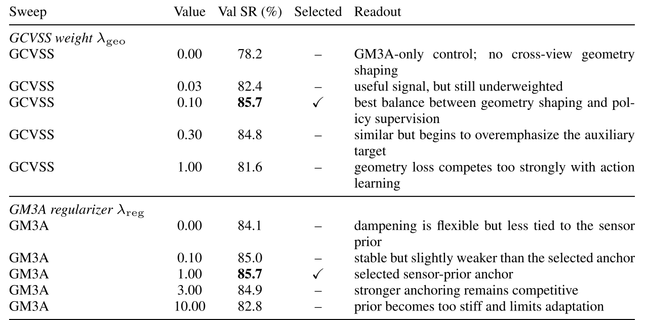
Complete original Table 17: Hyperparameter sweep for the reported loss weights. Validation success rates (%) on RLBench PerAct-18 under mild-noise evaluation with the fixed NISE stack.
Table 17: Hyperparameter sweep for the reported loss weights. Validation success rates (%) on RLBench PerAct-18 under mild-noise evaluation with the fixed NISE stack.
Accessible table, original values and citation links
Sweep Value Val SR (%) Selected Readout
GCVSS weight λgeo\lambda_{\mathrm{geo}}
GCVSS 0.00 78.2 – GM3A-only control; no cross-view geometry shaping
GCVSS 0.03 82.4 – useful signal, but still underweighted
GCVSS 0.10 85.7 ✓\checkmark best balance between geometry shaping and policy supervision
GCVSS 0.30 84.8 – similar but begins to overemphasize the auxiliary target
GCVSS 1.00 81.6 – geometry loss competes too strongly with action learning
GM3A regularizer λreg\lambda_{\mathrm{reg}}
GM3A 0.00 84.1 – dampening is flexible but less tied to the sensor prior
GM3A 0.10 85.0 – stable but slightly weaker than the selected anchor
GM3A 1.00 85.7 ✓\checkmark selected sensor-prior anchor
GM3A 3.00 84.9 – stronger anchoring remains competitive
GM3A 10.00 82.8 – prior becomes too stiff and limits adaptation

Note: The listed coefficients are the applied loss weights; λreg\lambda_{\mathrm{reg}} multiplies the unweighted regularizer once in the total training loss.

Concept demonstration

Open image ↗