Overview
LILIE learns an invertible image transform by captioning noise-corrupted features, then freezes the transform to provide an additional loss for pixel-space image generation.
At a glance
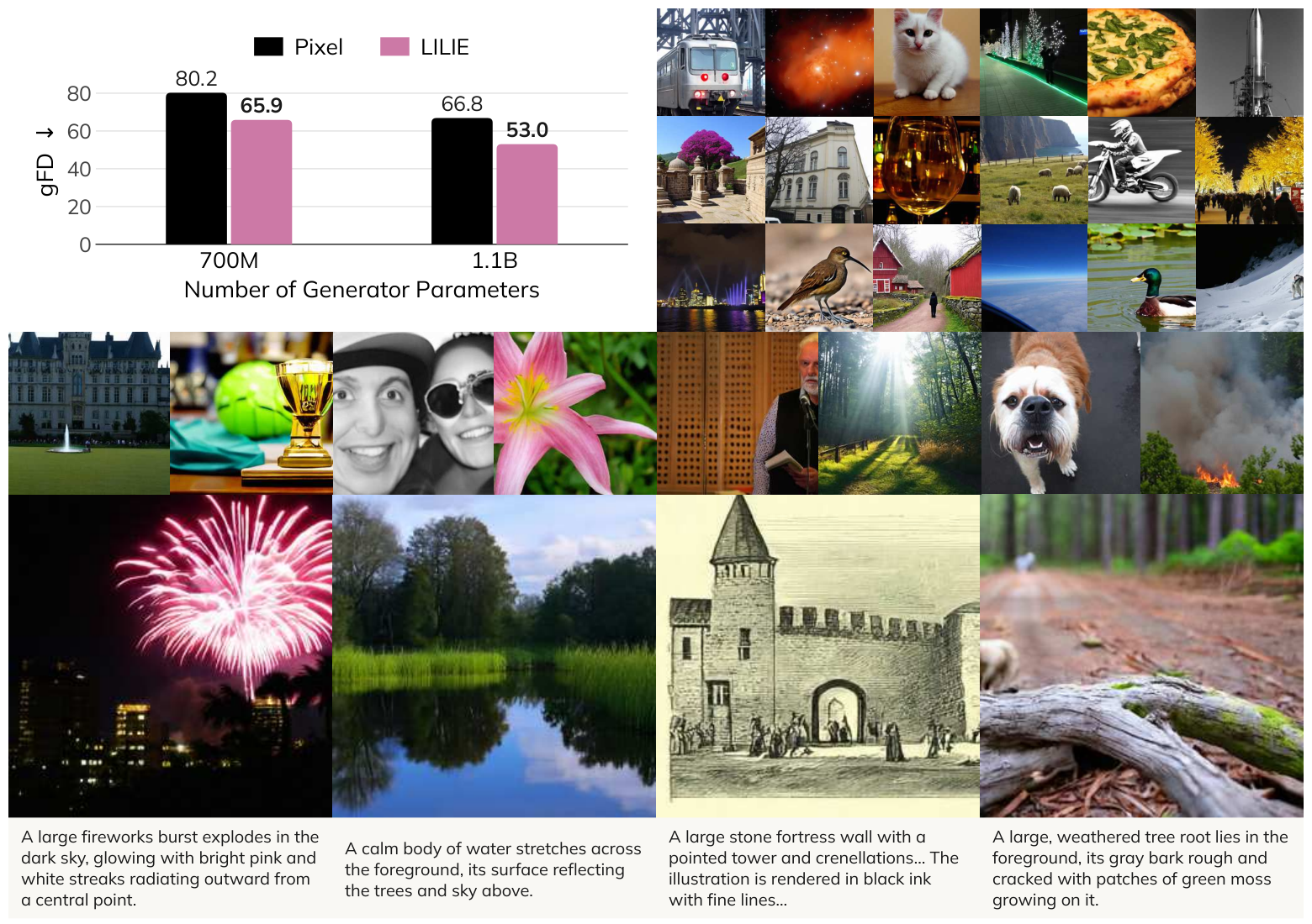
Language-Informed and Lossless Image Encoder learns a bijection with the same dimensionality as its image input. A vision–language model supplies caption-prediction supervision during encoder training; the frozen encoder then measures errors between a generator’s image prediction and its target. On GPIC at 256-by-256 resolution, the 1.1-billion-parameter generator improves its DINOv2-feature Fréchet distance from 66.84 to 53.01 when adding LILIE to pixel loss. These results concern one dataset, resolution, and generator family; an invertible representation is not itself a guarantee of semantic correctness or a lossless image-compression system.
1 Introduction
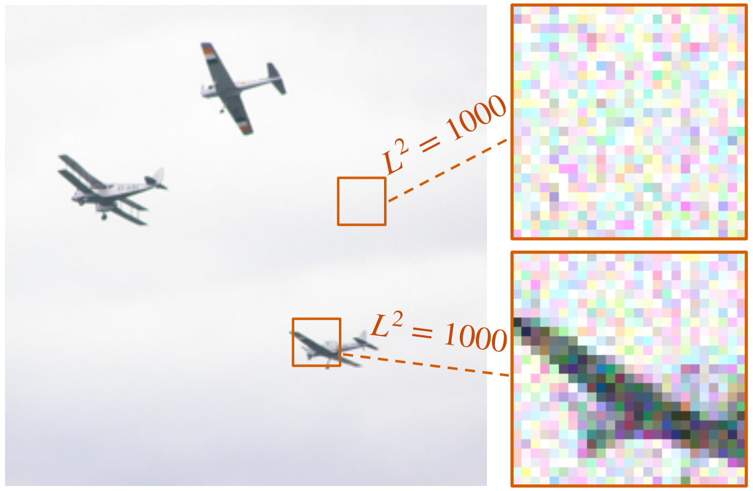
Pixelwise squared error assigns equal cost to perturbations with different semantic effects. LILIE learns a different geometry: caption-relevant information must remain recoverable after noise is added to an invertible image transform. The encoder keeps all image dimensions, while caption prediction shapes which errors become costly. The downstream generator still predicts pixels; LILIE is a training loss and does not become a mandatory decoding stage at sampling time.
2 Related Work
The work connects pixel-space diffusion, neural perceptual losses, invertible architectures, and caption-supervised representation learning.
Pixel-space diffusion.
Pixel-space generators avoid a separate lossy image tokenizer. LILIE builds on JiT and keeps the generator architecture fixed while changing its training signal, rather than attributing improvements to a new sampling or denoising architecture.
Feature-space losses for generation.
Perceptual losses compare predicted and target images through pretrained features. PixelGen combines such features with pixel-space supervision, while representation-alignment methods supervise hidden states. LILIE learns an invertible feature space specifically for the output-image loss; it is distinct from aligning the denoiser’s internal activations.
Invertible networks.
The encoder uses the invertible autoregressive transformer design from BiFlow. Its architecture is a normalizing-flow-style bijection, but its objective is caption cross-entropy, not a likelihood or density-modeling objective.
Language-supervised visual representations.
Language-supervised vision methods use contrastive alignment, caption prediction, or both. LILIE uses caption cross-entropy as its only encoder-training loss. Its supervision still depends on a pretrained vision–language model; “language-only” describes the new training objective, not the absence of externally pretrained components.
3 Methodology
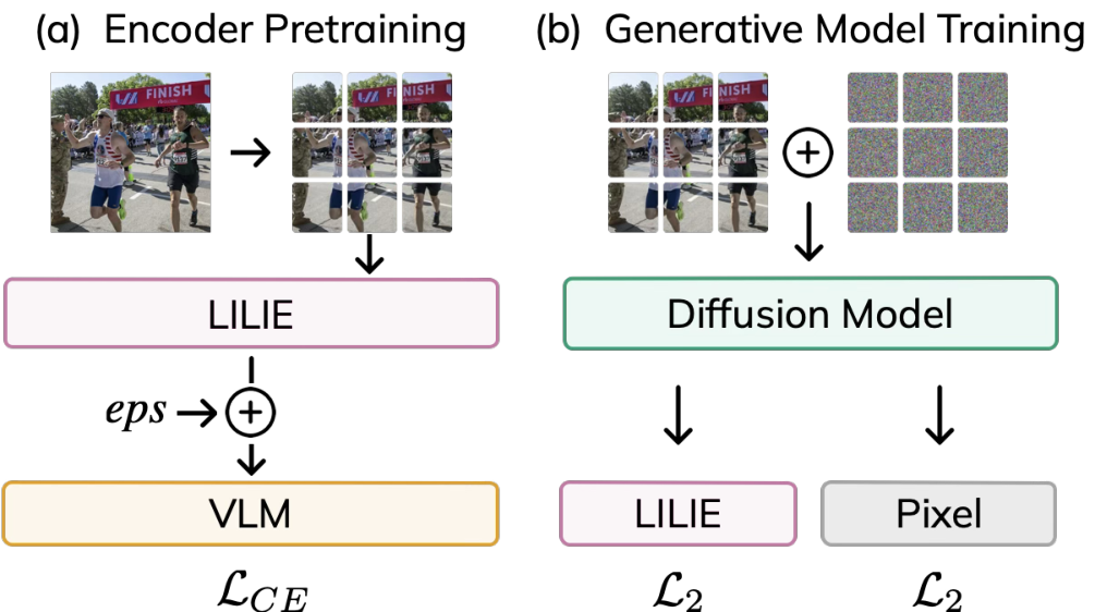
Training has two stages. First, jointly update an invertible image encoder and adapters in a captioning model using noisy encoded images. Then discard the captioning model, freeze the encoder, and use feature-space squared error alone or alongside pixel loss to train a text-conditioned generator.
3.1 LILIE: A Language-Informed and Lossless Image Encoder
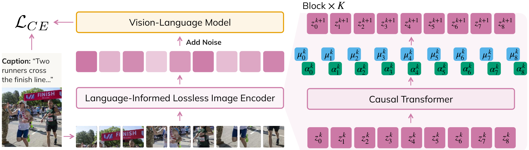
LILIE maps an image to an equally shaped tensor using invertible affine blocks. Corruption encourages caption-relevant content to remain recoverable; invertibility prevents the underlying encoder from discarding dimensions of the image.
Learning an invertible map.
Each encoded training image is normalized to root-mean-square magnitude one-half, corrupted by Gaussian noise, and captioned by a LoRA-adapted SmolVLM. Caption cross-entropy updates the encoder and LoRA weights. Per-image normalization prevents the encoder from defeating noise by simply scaling up all outputs. A moving estimate of the raw features’ second moment is recorded for later use. The noisy normalized captioning input is not itself invertible; the underlying encoder is, and downstream scaling uses a fixed corpus statistic to preserve that property.
Input: Image-caption batches data, initial invertible encode, pretrained vlm with LoRA, noise level sigma, EMA decay beta.
Output: Trained encode and second moment m2.
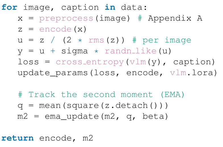
Input: Frozen encode and m2 from Algorithm 1; target x, prediction x_pred, time weight w(t), loss weight lambda.
Output: Generator training loss.
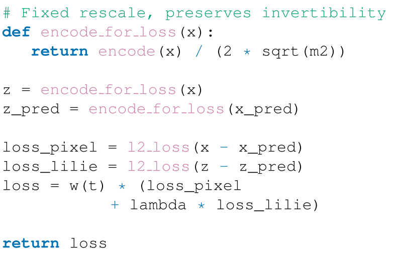
3.2 Training a T2I Generative Model with LILIE
The frozen encoder supplies an image comparison loss for a generator that continues to predict clean pixels.
Base objective.
JiT-T2I conditions on a frozen Qwen3-1.7B text encoder and trains with its clean-image form of the flow-matching objective. Captions are dropped for ten percent of training examples to support classifier-free guidance. LILIE does not remove the generator’s language-conditioning model.
Equation
Augmenting with LILIE.
For downstream loss, encoder outputs are divided by twice the square root of the stored corpus second moment, a fixed nonzero rescaling. The target and predicted image are compared in that space with the same time-dependent weighting as the base objective. The paper tests a LILIE-only objective and pixel loss plus a weighted LILIE term. Exact feature equality implies exact input equality under the bijection, but finite training errors and numerical conditioning still matter.
Equations 1
| (1) |
4 Experiments
Experiments compare loss choices while holding each generator’s architecture and training schedule fixed. Encoder pretraining adds a separate cost beyond the generator training budget.
4.1 Experimental Setup
The setup controls the downstream dataset and generator schedule, tunes loss/noise settings on validation data, and reports test metrics with independently selected guidance scales.
Data.
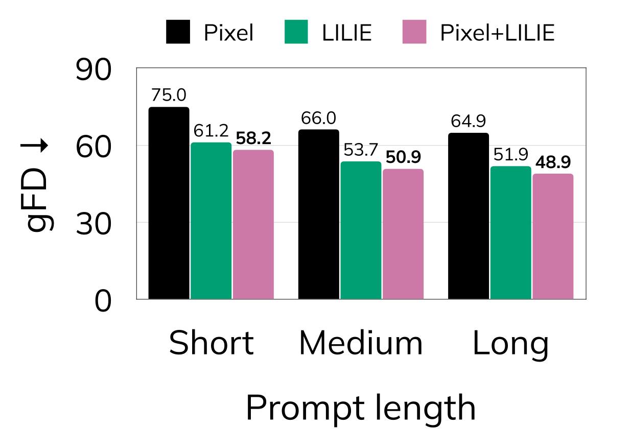
Encoder and generator training use GPIC image–caption pairs at 256-by-256 resolution. A full epoch has one hundred million examples and about 390,600 steps at batch 256. Caption lengths fall into tag, short, medium, and long categories, each with a corresponding encoder-training prompt.
Encoders.
The default 32-million-parameter LILIE-S has four affine blocks with four transformer layers each, width 384, and patch size sixteen. SmolVLM-256M uses rank-sixty-four LoRA adapters. Encoder training reportedly takes about forty hours on TPU v5e-32; this cost is separate from training the generator.
Generative models.
The two JiT-T2I generators have approximately 700 million and 1.1 billion parameters and share a frozen Qwen3-1.7B text encoder. Main results use one GPIC epoch, selected longer runs use two, and ablations use two hundred thousand steps. Reported generator times are twenty-seven and forty hours on TPU v6e-16, respectively.
Perceptual loss baselines.
Baselines use one feature loss at a time from VGG16 LPIPS, DINOv2, or SigLIP 2, with representation alignment disabled. Combined objectives use the paper’s specified perceptual metrics and time gate; feature-only experiments remove pixel loss and the gate and use squared feature distance for DINOv2/SigLIP 2. Thus the feature-only failures should be interpreted under these particular implementations.
Evaluation.
Quality, precision, recall, density, coverage, and squared maximum mean discrepancy are measured in DINOv2 space. Guidance is chosen separately for each model on Validation-50K, then evaluated on Test-50K with fifty Euler steps unless varied. The Fréchet metric measures distributional feature similarity and is not a direct test of prompt correctness, human preference, or every visual detail.
Hyperparameter selection.
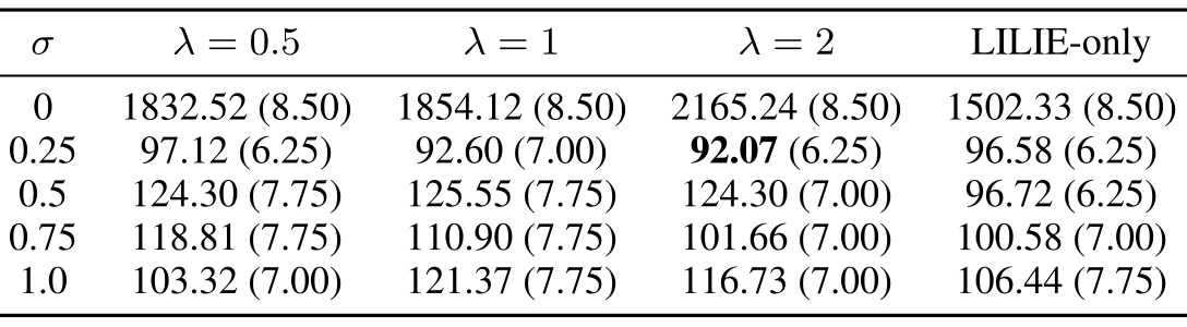
A validation sweep tests five encoder-noise levels and three mixed-loss weights, plus feature-only loss, using the smaller generator at two hundred thousand steps. Noise standard deviation 0.25 and LILIE weight two are selected for the main runs. The main conclusions depend on this tuning rather than on an arbitrary noise scale.
4.2 Generation Results
LILIE improves distributional generation metrics over pixel-only training, while separate alignment benchmarks and perceptual-loss comparisons provide a more qualified picture.
LILIE improves generation quality.
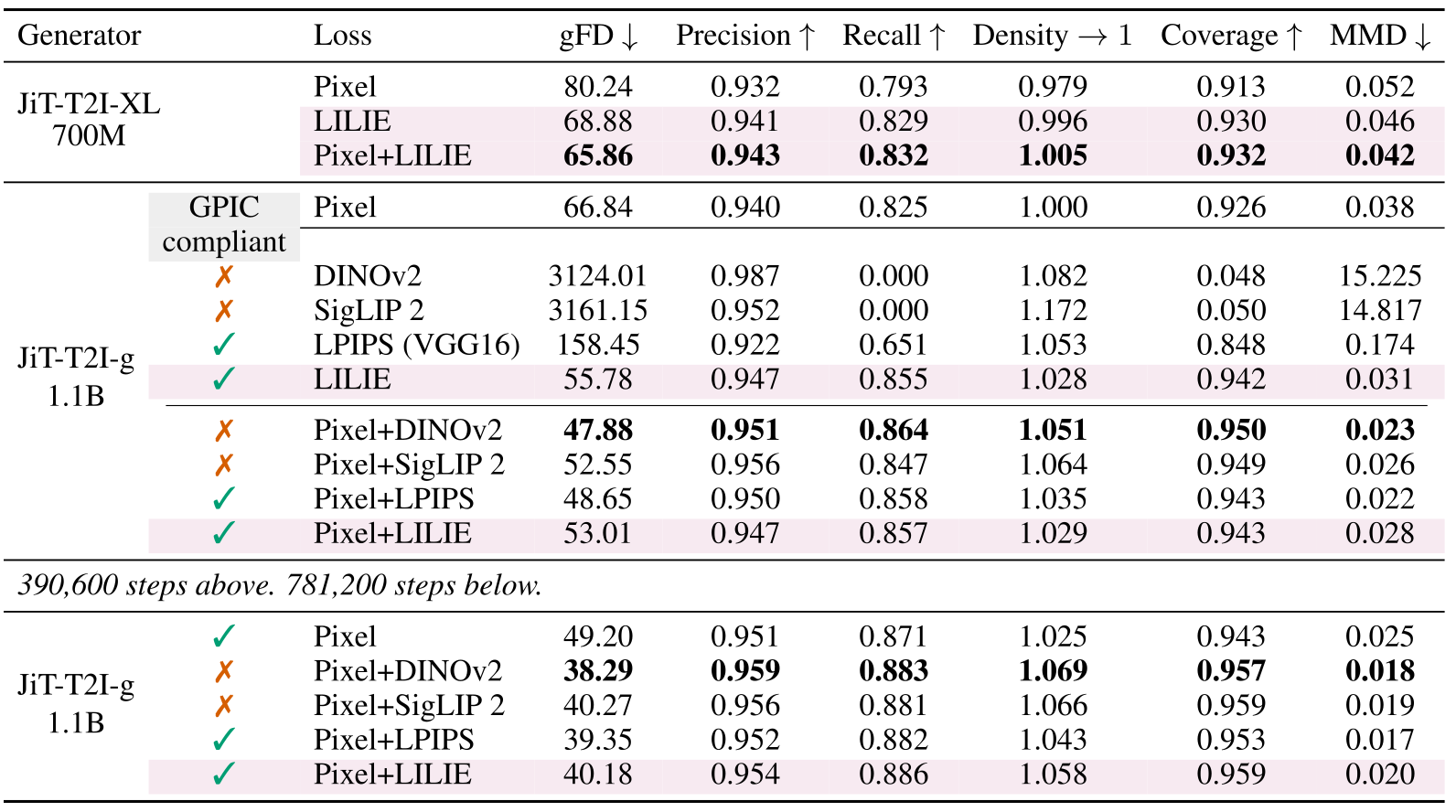
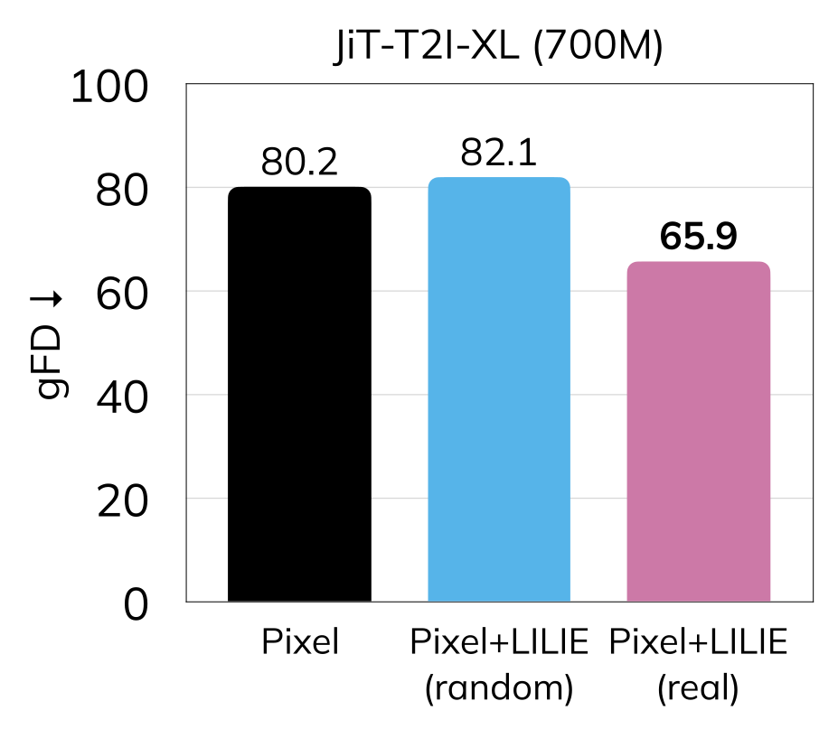
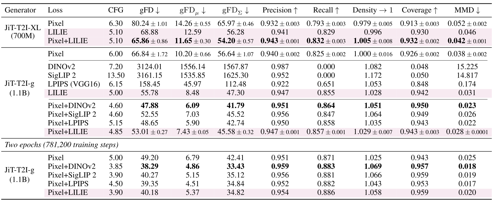
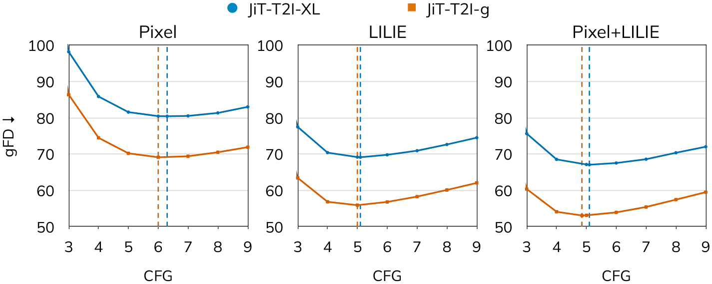
Adding LILIE improves test Fréchet distance from 80.24 to 65.86 for the 700-million-parameter generator and from 66.84 to 53.01 for the larger model, alongside improved precision and recall. For these one-epoch pixel and mixed configurations, the appendix reports three trials: the larger-model values are 66.84±1.72 versus 53.01±0.27, using sample standard deviations. Most other comparisons are single runs.
At two epochs, the larger model improves from 49.20 to 40.18. LILIE is competitive with, but does not dominate, all perceptual losses: pixel+LPIPS reaches 48.65 at one epoch and 39.35 at two, while pixel+DINOv2 reaches 47.88 and 38.29 under different pretraining/protocol conditions.
LILIE loss can be used on its own.
LILIE alone reaches 68.88 and 55.78 at the two model sizes, improving over pixel-only training. The tested DINOv2- and SigLIP-only losses give severely degenerate distributions with zero recall, while LPIPS alone is also much worse at 158.45. The invertible feature map gives a uniquely identifying target when matched exactly, although that mathematical property alone does not establish why every finite optimization run will succeed.
Language supervision matters.
Randomizing encoder-training caption tokens while preserving lengths and prompts gives downstream Fréchet distance 82.06, versus 80.24 for pixels and 65.86 for real-caption LILIE. The generator still trains on genuine captions. This supports the role of informative language in learning the loss rather than an effect from simply adding an invertible network.
4.3 Sampling Steps
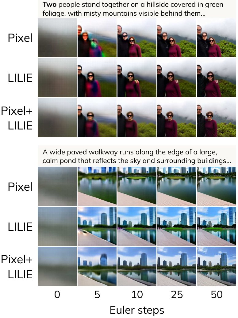
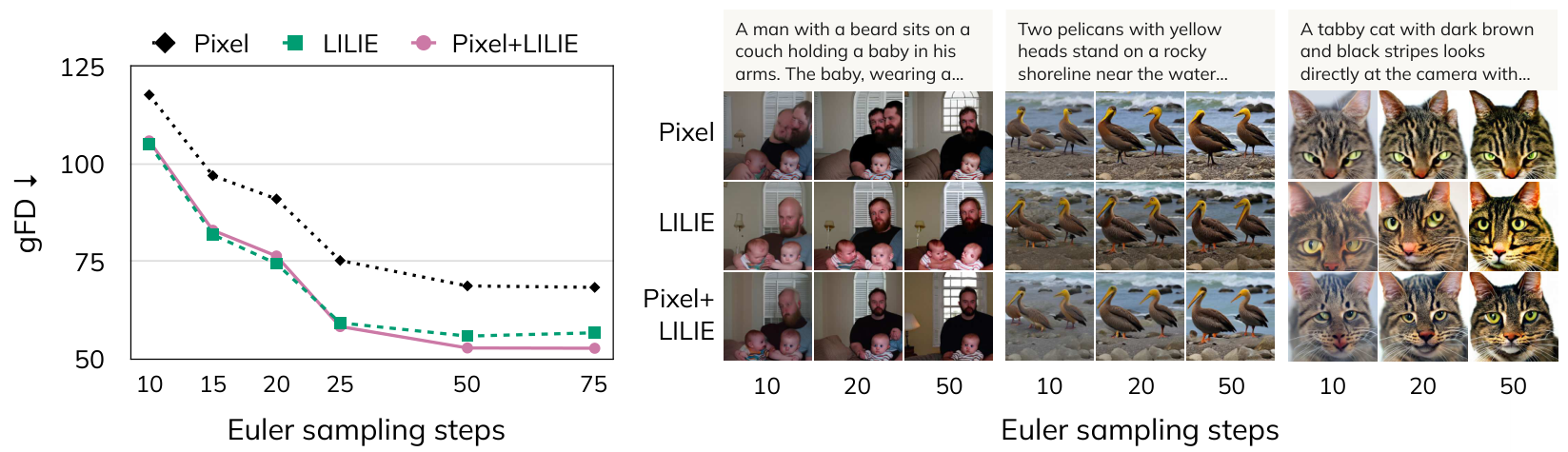
At the tested sampling budgets, pixel+LILIE has lower Fréchet distance than pixels. Twenty-five mixed-loss steps reach 58.23, below the pixel model’s fifty-step 68.67 in this sweep. These sweep values differ from the main table’s three-trial means. Gains beyond fifty steps are small; LILIE-only actually worsens from 55.78 to 56.63 at seventy-five steps. Guidance chosen at fifty steps is held fixed, so the sweep does not retune every method at every budget.
4.4 Encoder Size and Data Scaling
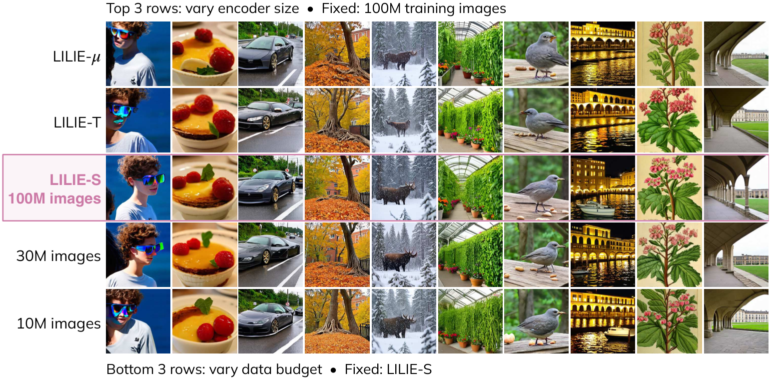
The size/data ablations keep generator training fixed at two hundred thousand steps and vary the separately trained encoder. More encoder capacity or training data generally improves Fréchet distance within the tested range, with smaller metric-specific exceptions.
Model size.
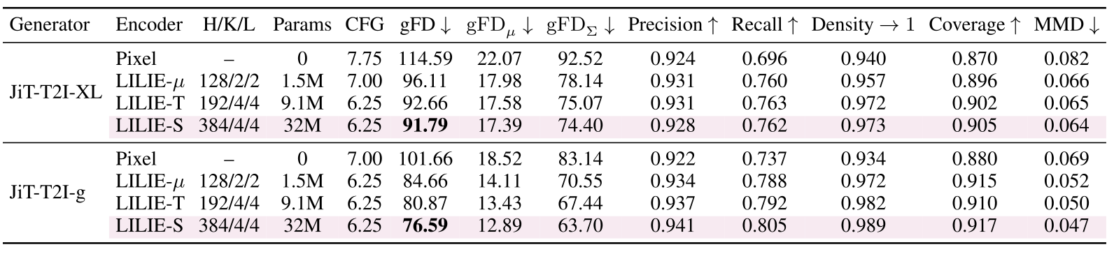
Micro, tiny, and small encoders have 1.5, 9.1, and 32 million parameters. With the larger generator, their Fréchet distances are 84.66, 80.87, and 76.59, compared with pixel-only 101.66. Even the micro encoder helps. These values come from shorter generator training and should not be compared directly with the main full-epoch scores.
Training data.
Training LILIE-S on ten, thirty, and one hundred million images reduces the larger generator’s Fréchet distance from 83.01 to 81.18 to 76.59; the smaller generator improves from 97.79 to 93.52 to 91.79. Increased encoder training therefore helps at a fixed generator budget, but increases total system training compute.
5 Discussion and Conclusion
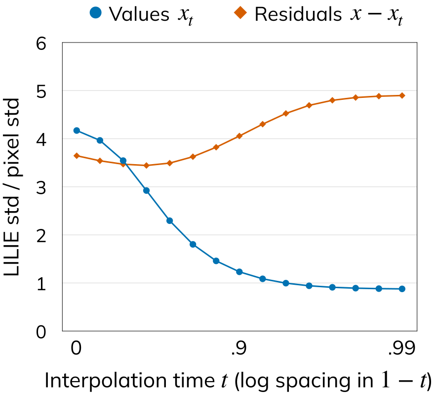
The learned feature loss amplifies some small near-data perturbations: at interpolation time 0.99, the reported residual standard deviation is about 4.9 times that in pixel space despite similar overall feature scale. This describes a measured sensitivity of the learned representation, not a universal guarantee that every amplified error is semantically important.
Comparisons with pretrained perceptual losses.
Combined perceptual losses are strong competitors, and LILIE is not uniformly the best metric score. DINOv2 and SigLIP 2 have different, much larger pretraining distributions that may overlap GPIC test data; DINOv2 is also the evaluation feature extractor. The authors label these useful representation comparisons but not controlled GPIC-protocol-compliant experiments. LPIPS remains a protocol-compliant strong baseline. Combining LILIE with multiple perceptual losses is left untested.
| Loss | Supervised | SSL | Language | Training images | Not distilled | GPIC compliant |
|---|---|---|---|---|---|---|
| DINOv2 | - | ✓ | - | 142M | ✗ | ✗ |
| SigLIP 2 | - | ✓ | ✓ | 10B | ✗ | ✗ |
| LPIPS (VGG16) | ✓ | - | - | 1.28M | ✓ | ✓ |
| LILIE | - | - | ✓ | 100M | ✓ | ✓ |
A simple language-informed loss for visual generation.
A compact invertible encoder trained through language can provide useful supervision for pixel-space generation, either alone or with pixel loss. The reported gain does not require the encoder or captioning model during generator sampling. Released code, encoders, and generator weights are referenced in the original paper.
Acknowledgements.
The authors acknowledge feedback from Stanford Vision Lab and the CogAI group.
Appendix
The appendix retains all training configurations, supplementary metrics, noise/loss sweeps, limitations, exact captioning prompts, and complete qualitative sample grids.
Appendix A Additional Training Details
Implementation details explain preprocessing, noisy vision–language inputs, and the invertible transformer architecture.
preprocess in Algorithm 1 .
Images are resized with antialiased bicubic interpolation so the shorter side is 256 pixels, center-cropped to 256-by-256, and mapped from byte intensities to the interval minus one to one. These preprocessing operations define the image domain being modeled; the claim of invertibility concerns the subsequent encoder, not recovery of discarded crop or resize information.
SmolVLM input.
Noise-corrupted features replace image input to SmolVLM and are not clipped to the usual image-value interval. LoRA adaptation lets the captioning model handle these inputs. Clipping would discard information and change the training procedure.
A.1 Encoder Architecture
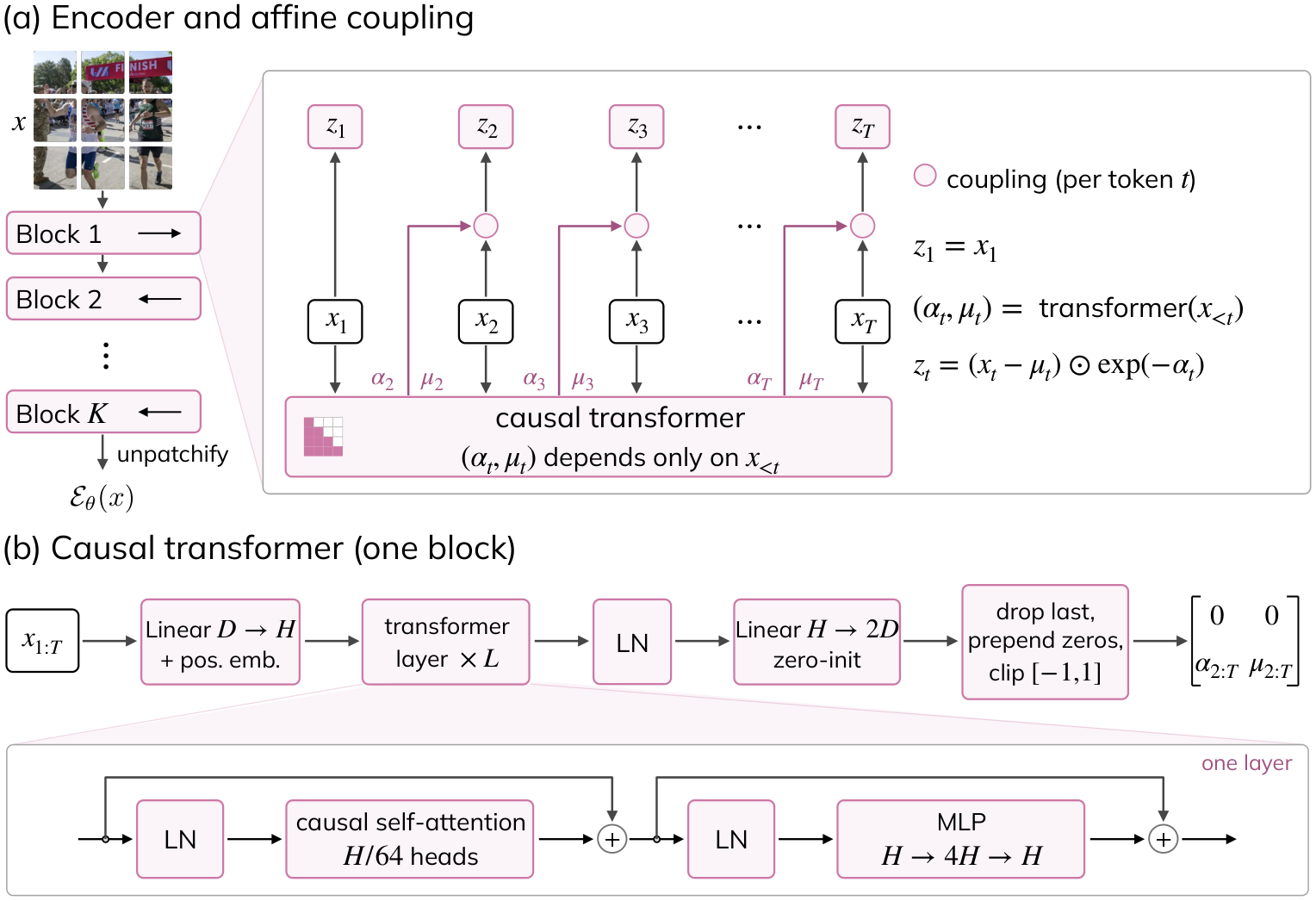
Images are patchified and passed through a stack of autoregressive affine blocks with alternating patch orders, then reassembled to the original tensor shape. The original architectural diagram retains all scale/shift operations and transformer internals.
Block parameters.
For each patch, the affine log-scale and shift depend only on preceding patches in the block’s order and are clipped to minus one through one. The first patch passes through unchanged. This causal structure supports inversion; it does not make the transform a dimensionality-reducing tokenizer.
Transformer internals.
Each block projects patches to the bottleneck width, adds positional embeddings, and applies causal transformer layers with width divided by sixty-four attention heads and a fourfold feedforward expansion. A zero-initialized final head produces scale and shift values. Dropping its last position and prepending zeros ensures that each patch’s transformation uses only earlier patches.
Appendix B Experimental Details
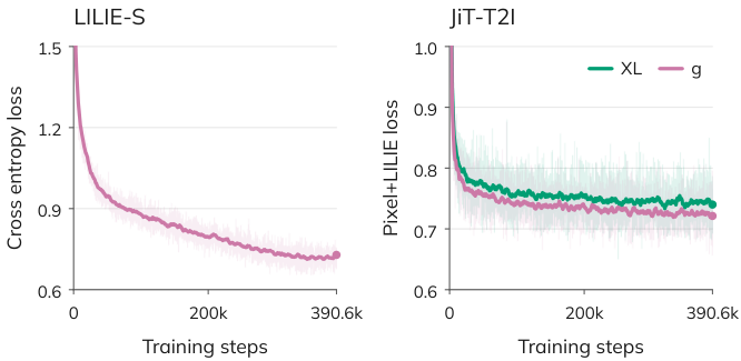
The appendix retains full generation metrics and guidance choices, encoder/generator configurations, and training curves. Three-trial means and sample standard deviations apply to the one-epoch pixel and pixel+LILIE settings at both sizes, rather than every table entry. Main runs use 390,600 steps; selected two-epoch runs use 781,200.
| LILIE- | LILIE-T | LILIE-S | |
| architecture | |||
| flow backbone | Improved TARFlow (Zhai et al., 2025; Lu et al., 2026b) | ||
| blocks | 2 | 4 | 4 |
| layers per block | 2 | 4 | 4 |
| bottleneck dim | 128 | 192 | 384 |
| heads | 2 | 3 | 6 |
| parameters | 1.5M | 9.1M | 32M |
| image size | 256 | ||
| patch size | 16 | ||
| coupling clip range | 1.0 | ||
| VLM | SmolVLM-256M (Marafioti et al., 2025) | ||
| LoRA (Hu et al., 2022) rank | 64 | ||
| LoRA | 32 | ||
| LoRA targets | all linear layers except the output head | ||
| max caption tokens | 256 | ||
| training | |||
| training steps | 390,600 (1 epoch on GPIC Full) | ||
| warmup steps | 20,000 | ||
| optimizer | AdamW (Loshchilov and Hutter, 2019), | ||
| batch size | 256 | ||
| flow learning rate | 1.2e-3 | 8e-4 | 4e-4 |
| VLM learning rate | 4e-4 | ||
| learning rate schedule | linear warmup, cosine decay to 1e-6 | ||
| weight decay | 1e-4 | ||
| gradient clipping | AutoClip (Seetharaman et al., 2020), 10th percentile | ||
| noise level | 0.25 | ||
| feature RMS target | 1/2 | ||
| ema decay for | 0.99 | ||
| JiT-T2I-XL | JiT-T2I-g | |
| architecture | ||
| depth | 24 | 16 |
| hidden dim | 1024 | 1536 |
| heads | 16 | 24 |
| bottleneck | 128 | 256 |
| parameters | 700M | 1.1B |
| image size | 256 | |
| patch size | 16 | |
| text encoder | Qwen3-1.7B (Yang et al., 2025), frozen | |
| max caption tokens | 300 | |
| training | ||
| training steps | 200K (ablations), 390,600, 781,200 | |
| warmup steps | 4,000 | |
| optimizer | AdamW (Loshchilov and Hutter, 2019), | |
| batch size | 256 | |
| learning rate | 1e-4 | |
| learning rate schedule | constant | |
| weight decay | 0 | |
| gradient clipping | 1.0 | |
| ema decay | 0.9999 | |
| time sampler | , , | |
| noise scale | 1.0 | |
| clip of in division | 0.05 | |
| caption drop (for CFG) | 0.1 | |
| sampling | ||
| ODE solver | Euler | |
| ODE steps | 50 | |
| time steps | linear in [0.0, 1.0] | |
| CFG scale (Ho and Salimans, 2022) | selected on GPIC Validation-50K | |
| weights | EMA | |
B.1 Additional Benchmarks
On GenEval, mixed loss gives 36.41±1.32 overall versus pixel-only 33.57±1.38, with standard errors over prompts. LILIE-only gives 32.49±1.32, and mixed loss lowers the two-object score from 28.28 to 24.24 despite improving some other categories. DPG-Bench overall changes modestly from 73.00±0.63 to 73.63±0.61; LILIE-only is 72.86±0.61. These results do not establish uniform compositional or language-alignment improvements. GenEval removes the leading “a photo of” phrase for all three configurations.
| Loss | Overall | Single | Two | Counting | Colors | Position | Color attr. |
|---|---|---|---|---|---|---|---|
| Pixel | 33.571.38 | 67.504.34 | 28.283.26 | 14.692.42 | 53.724.21 | 18.002.78 | 19.252.79 |
| LILIE | 32.491.32 | 62.504.00 | 26.523.17 | 14.062.63 | 56.124.03 | 13.002.32 | 22.752.80 |
| Pixel+LILIE | 36.411.32 | 77.503.57 | 24.243.16 | 15.622.68 | 56.123.89 | 23.753.02 | 21.252.92 |
| Loss | Overall | Global | Entity | Attribute | Relation | Other |
|---|---|---|---|---|---|---|
| Pixel | 73.000.63 | 76.602.31 | 82.210.56 | 86.590.53 | 92.300.58 | 70.002.91 |
| LILIE | 72.860.61 | 76.902.29 | 82.130.58 | 86.250.54 | 91.680.60 | 64.403.07 |
| Pixel+LILIE | 73.630.61 | 79.332.15 | 82.490.57 | 86.150.53 | 92.500.57 | 68.802.89 |
B.2 Implementation of Perceptual Loss Baselines
Perceptual baselines train generators from scratch with one auxiliary feature model and no hidden-state representation alignment. Their loss definitions and time gating are preserved for reproducibility.
LPIPS.
The LPIPS baseline uses the standard pretrained VGG16 implementation.
DINOv2 and SigLIP 2.
DINOv2 and SigLIP 2 provide 256 patch tokens of width 768, with SigLIP features taken before pooling. Combined pixel objectives use average patch cosine dissimilarity; feature-only objectives use normalized squared feature distance. The paper retains both formulas.
Equation
Aggregate form and time gating.
Mixed perceptual loss is enabled only after interpolation time 0.3, with weights 0.1 for LPIPS and 0.01 for DINOv2/SigLIP 2. Feature-only runs use unit weight and remove both pixel loss and the time gate. These baseline settings differ from LILIE’s default weight two and should be included when interpreting the comparison.
Equation
Appendix C Noise Level and Loss Weight
The full validation sweep preserves all twenty encoder-noise/objective combinations and their selected guidance scales. Zero-noise encoders produce very poor generation, with distances around 1,500–2,165, despite their invertible architecture. The best mixed setting is noise 0.25 and weight two, at validation distance 92.07; raising noise does not improve that best result. Guidance in this ablation uses a coarse five-value grid, whereas the final full-result table reports finer 0.05-scale selection.
Appendix D Model Size and Data Ablations
Full size/data tables include distributional-distance components, fidelity/diversity metrics, and guidance choices. Fréchet distance improves with the tested encoder scaling, but individual precision, recall, and coverage entries need not improve monotonically. All generators here have two hundred thousand steps, so these tables isolate encoder changes within that budget rather than total-compute matching.

Appendix E Limitations
All experiments use GPIC, 256-by-256 images, JiT-T2I generators, and SmolVLM-256M encoder supervision. The largest encoder is only 32 million parameters; larger captioning models, larger encoders, other domains/resolutions, and an optimal encoder-training-budget rule remain unexplored. Training requires captions and a pretrained vision–language model. The paper does not test mixtures of LILIE and other perceptual losses.
Appendix F Captioning Prompts
All four original system/user prompt pairs are preserved verbatim with indentation. They request unordered tags, one-to-two-sentence short captions, two-to-three-sentence medium captions, or five-to-seven-sentence detailed captions. These prompts are matched to GPIC’s caption-length labels during encoder training.
[tag]
system:
  Your goal is to write a compressed keyword-style caption (unordered tags)
  for the given image. The output must be a short, unordered list of tags
  describing the main visible content.
user:
  Write a keyword-style caption (tag-style) for the image shown.
[short]
system:
  Your goal is to write a short caption (1-2 sentences) that describes the
  given image in simple language that a middle school student can
  understand. The caption must be enough to identify the main subject and
  the basic setting/action.
user:
  Write a short caption (1-2 sentences) for the image shown.
[medium]
system:
  Your goal is to write a medium-length caption (2-3 sentences) that
  describes the given image in simple language that a middle school student
  can understand. The caption must be enough to identify the main subject
  and the basic setting/action.
user:
  Please write a caption (2-3 sentences) for the image shown.
[long]
system:
  Your goal is to write a long, highly detailed caption (5-7 sentences)
  that describes the given image in simple language that a middle school
  student can understand. The caption should include enough detail for them
  to understand what appears in the foreground and background and picture
  how the scene is arranged.
user:
  Please write a caption (5-7 sentences) for the image shown.
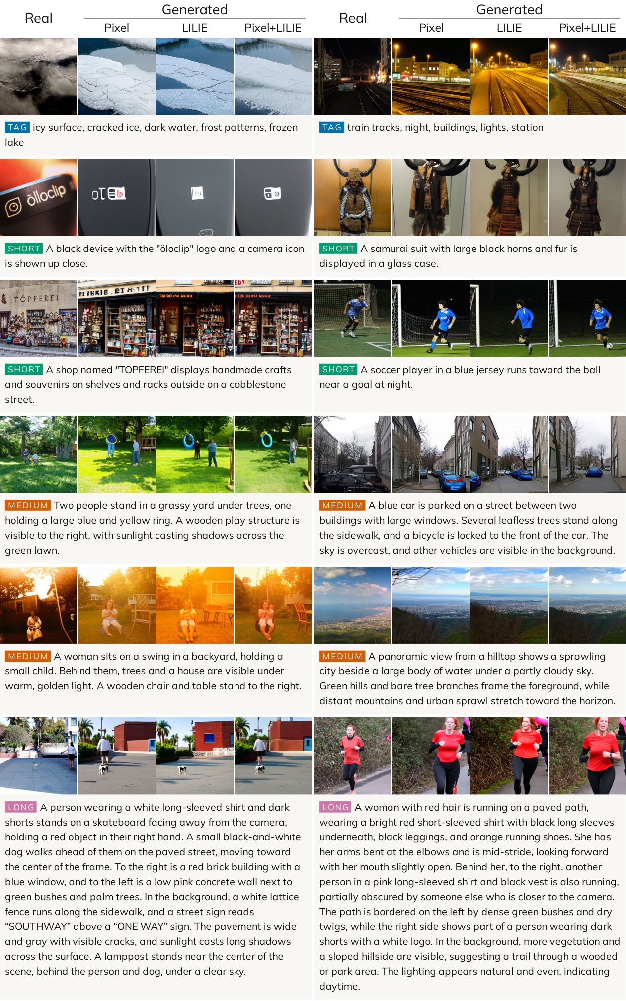
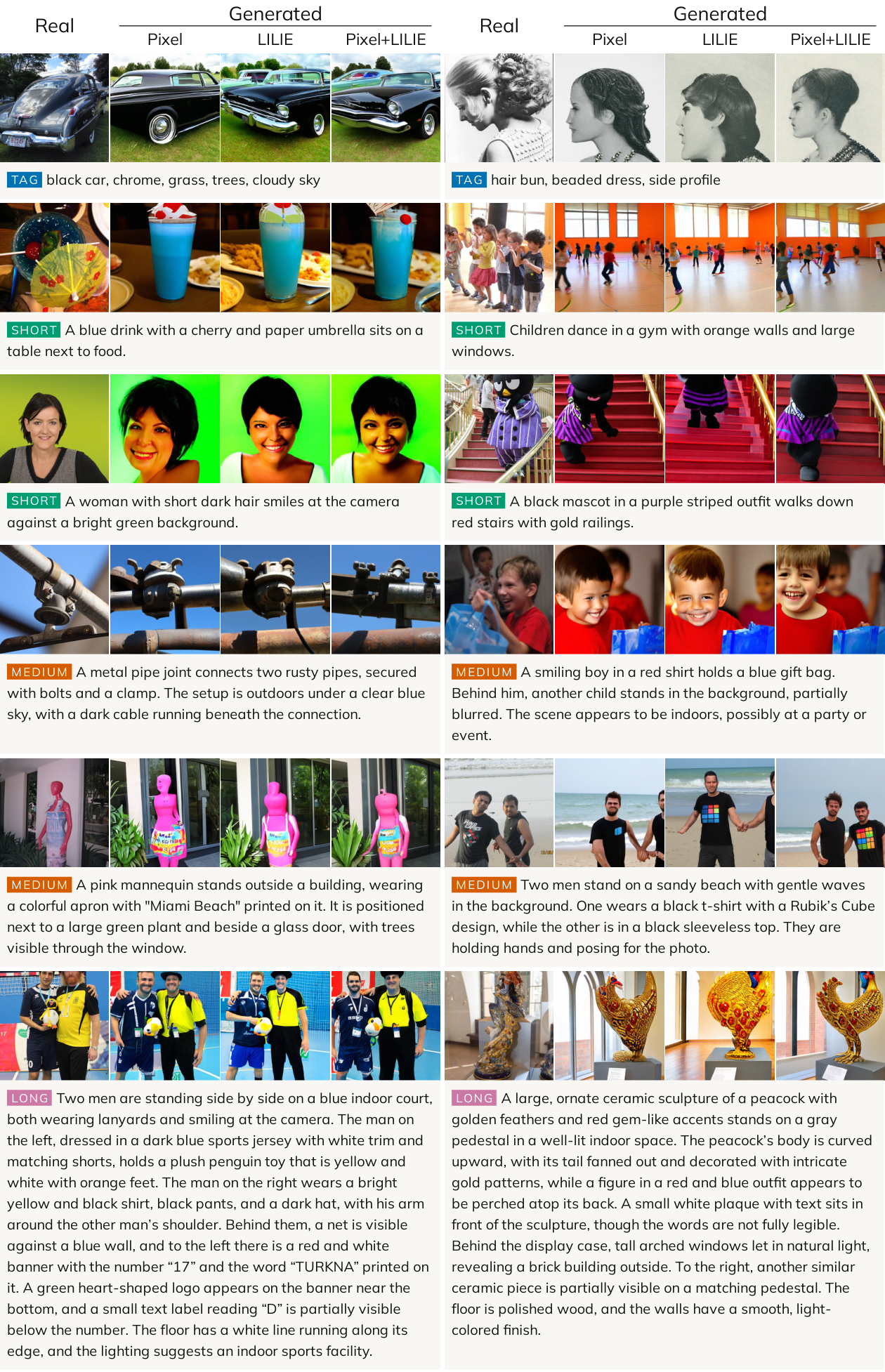
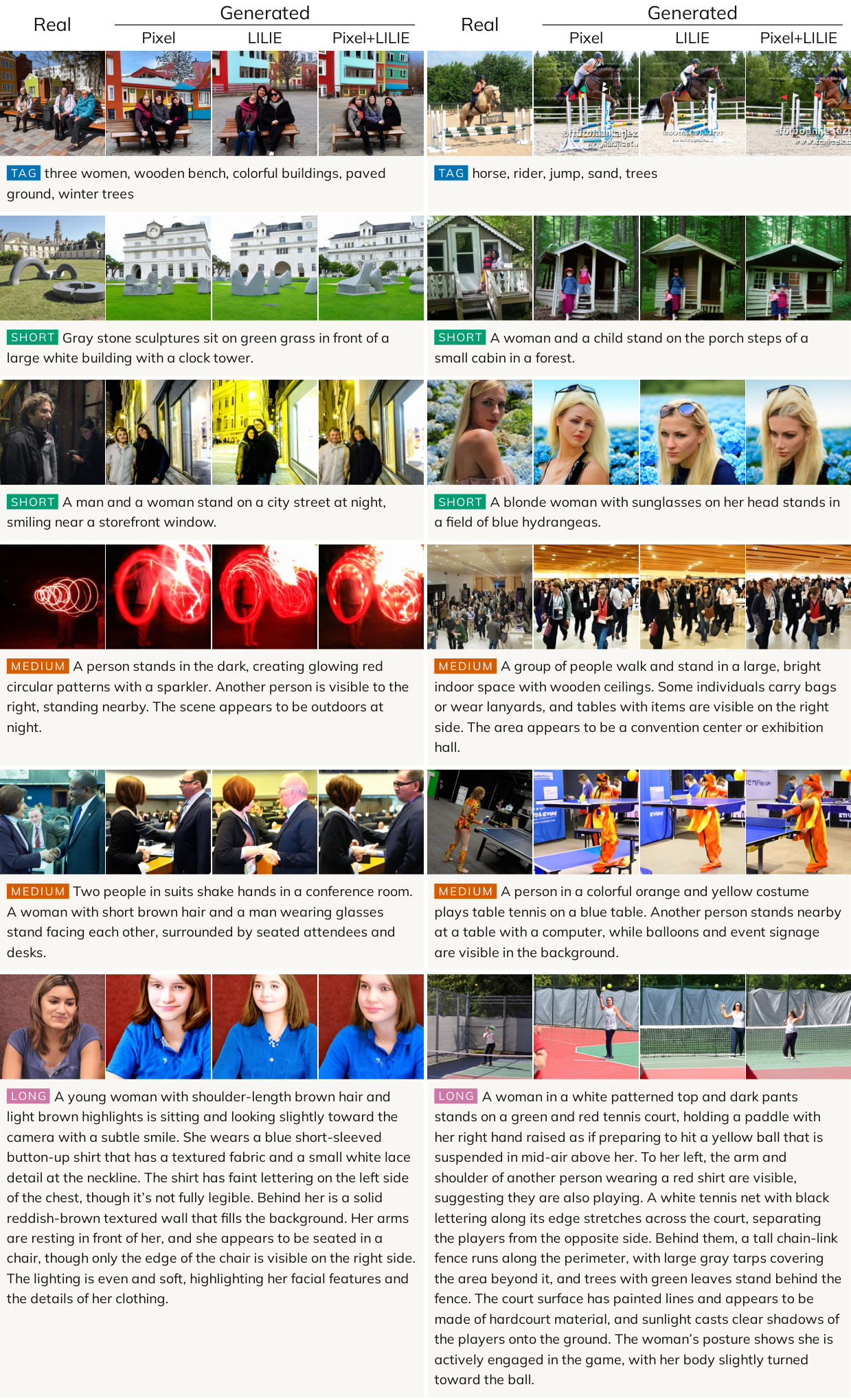
Appendix G Samples
The full appendix retains intermediate clean-image predictions along fifty-step trajectories, five grids of randomly selected held-out examples comparing real images and all three generation losses, and the selected lily mosaic. Each model uses its chosen guidance scale. Selected illustrations and random sample grids serve different evidential roles; neither replaces the quantitative test metrics.