Overview
This edition follows the 38-page arXiv v1 of 15 October 2026, including all 22 figures, 12 numbered tables, 16 equations, the algorithm and six appendices. It preserves full-resolution qualitative panels and restores six reduced HTML figures from native PDF art. Read the experiments as task-level world-model adaptation from observed interactions, with candidate action sets guaranteed to contain a successful option. The headline physical-error average combines different units and is not a single calibrated pixel-error measure.
At a glance
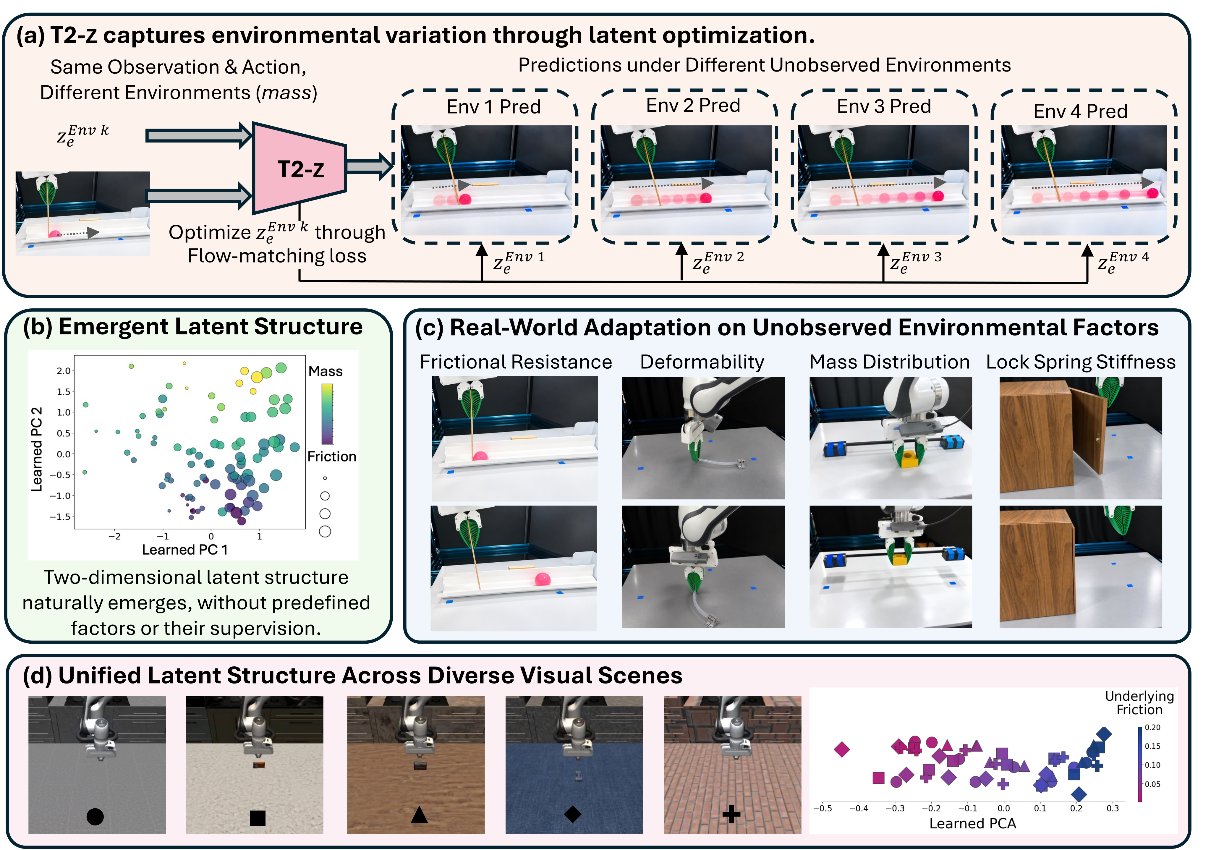
T2-z conditions a robotic video world model on a 32-dimensional environment vector. Alternating training fits shared dynamics with vectors fixed, then fits vectors with the model fixed; test-time adaptation changes only a new vector using observed interaction outcomes. Across seven simulation and four hardware settings, average action success rises from 33.73% to 72.96% relative to the non-adaptive model. The reported prediction-error reduction from 15.20 to 7.00 averages pixel, angle and lamp-score errors. One or two interaction trajectories suffice for the main task protocols, but this does not guarantee identifying arbitrary hidden dynamics.
1 Introduction
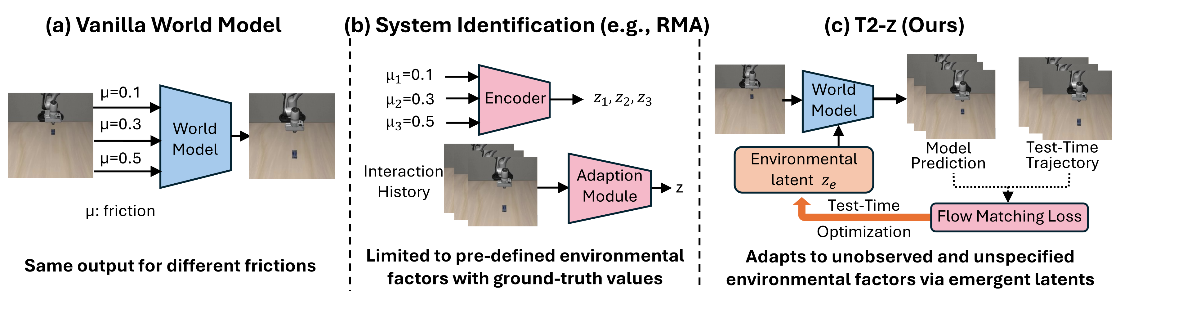
Visually similar scenes can respond differently because of hidden friction, mass or interaction rules. Optimizing a predictive latent offers an alternative to specifying numerical physical factors or learning a fixed history encoder. The latent is learned without factor-value labels, although training still groups trajectories by environment. Once adapted, it conditions predictions for new actions in that environment; it is not itself a policy or an explicit physical-parameter estimate.
2 Related Works
The approach connects action-conditioned world models with system identification and test-time adaptation. Rapid Motor Adaptation uses privileged factor supervision and a history-to-embedding model; T2-z instead fits its vector through video-prediction error. It builds on BWM and the Wan backbone. Other cited methods adapt policies, prompts, memory or world-model weights; this paper isolates a small environment representation while freezing the shared model at deployment.
3 Method
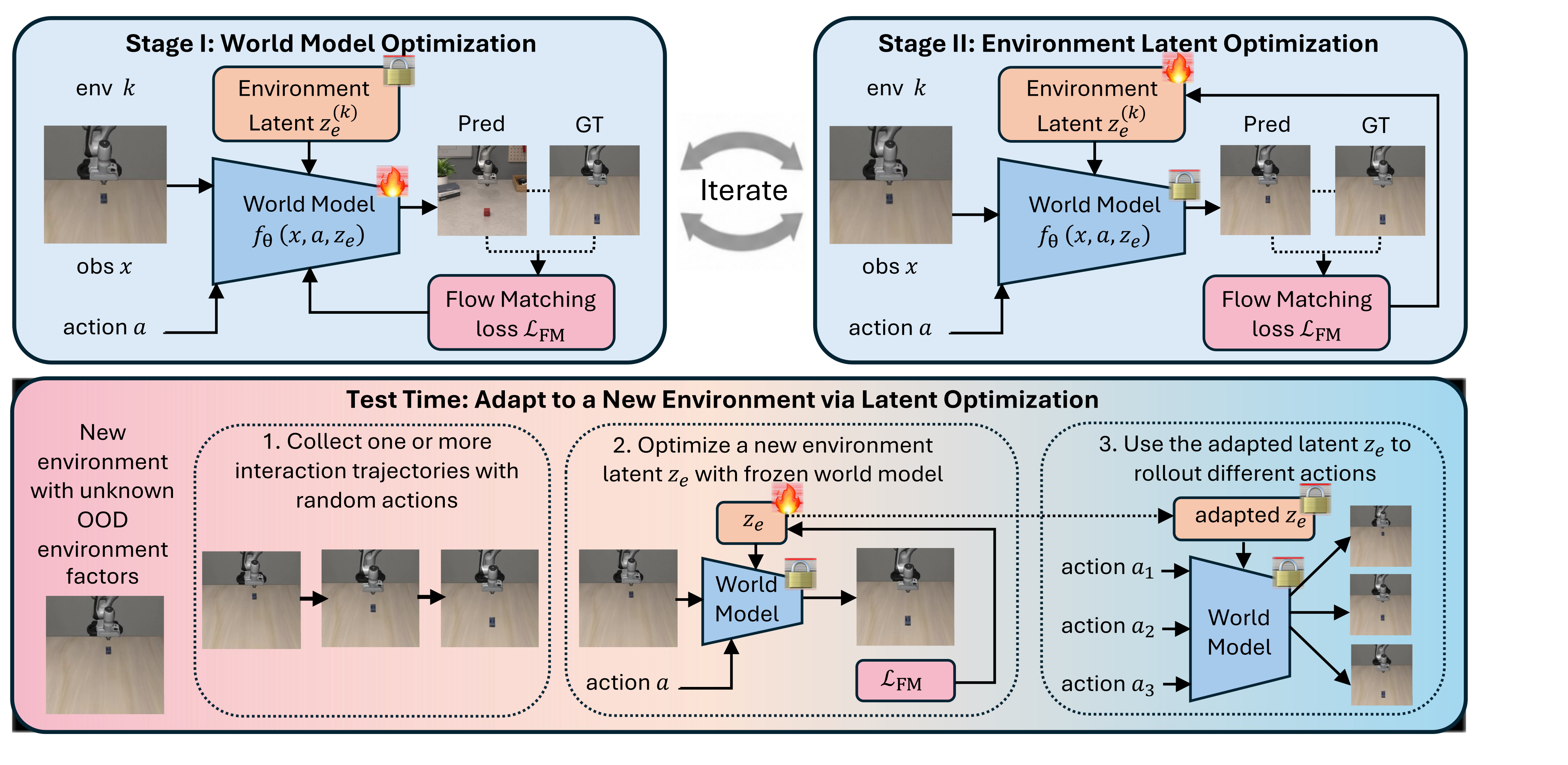
A shared flow-matching objective supports three operations: train the world model, train environment vectors, and fit a new vector at test time. Algorithm 1 preserves the exact alternating and deployment loops.
3.1 Problem Setup
The predictive distribution depends on the initial observation, action and environment latent. Flow matching trains the velocity of noisy/interpolated future video latents. No loss directly supervises which physical factor a latent coordinate should represent.
Equations 1–2
| (1) |
| (2) |
3.1.1 Training
Each training environment receives a vector initialized independently from the unit uniform distribution. Slow shared-model learning alternates with faster latent updates; environment identities associate multiple action trajectories with the same vector.
Equation 3
| (3) |
Stage I: World-Model Optimization.
Hold all environment vectors fixed while updating shared world-model weights across environments and actions. This phase learns predictive structure that can be reused across the training distribution.
Equation 4
| (4) |
Stage II: Environment-Latent Optimization.
Freeze shared weights and optimize the vector associated with each environment against its observed trajectories. Differences in action outcomes can then be explained only through the conditioning vector, within the representational capacity of the fixed predictor.
Equation 5
| (5) |
Alternating Optimization
Training begins with a model-only block, then alternates fixed-length latent and model blocks. Updated vectors inform subsequent model training; an improved model changes the prediction-error landscape used to fit those vectors.
3.1.2 Test-Time Optimization
For a held-out environment, collect one or more random-action interaction trajectories and optimize a freshly initialized vector while all shared weights remain frozen. A coarse-to-fine learning-rate schedule minimizes flow loss on those observations. Reuse the resulting vector for disjoint query actions; their outcomes do not enter adaptation. Variable interaction counts are supported by the objective, but successful extrapolation still depends on informative interactions and the learned model.
Equations 6–8
| (6) |
| (7) |
| (8) |
4 Experiments
Seven simulated settings and four physical tasks evaluate video prediction and action selection, with additional latent, optimization and compute studies.
4.1 Experimental Setup
All methods share task-level data, query inputs and candidate actions; adaptive methods receive the same interaction trajectories. Architecture and adaptation procedures differ.
Tasks
Simulation varies friction, gravity, collision mass, hidden light-switch rules, balance mass ratios, joint mass/friction and friction across 30 backgrounds. Hardware tasks vary a ball’s internal bead load, a door-latch spring, stick-end weights and soft-tube properties. These are controlled task families, not an unrestricted changing-world benchmark.
Implementation Details.
The BWM-initialized Wan2.2-TI2V-5B uses a 32-D latent. After 300 model updates, 200 latent and 200 model updates alternate at learning rates 0.03 and 10⁻⁵. Test time uses 40 latent updates: ten each at 3.0, 1.5, 0.5 and 0.15. Main evaluations use one interaction in seven settings and two in light-switch, mass-balance, door and stick tasks.
| Task | Method | Physical Error (Mean) | Physical Error (Final) | LPIPS | PSNR | Action Success |
|---|---|---|---|---|---|---|
| Mass Balance | Standard World Model | 1.1844 | 4.5571 | 0.0244 | 32.969 | 40.0% |
| LoRA TTA | 1.7975 | 7.3105 | 0.0631 | 24.895 | 50.0% | |
| DINOv2 Context | 1.2636 | 4.9480 | 0.0239 | 33.263 | 30.0% | |
| TTT-KQV | 2.5075 | 10.1759 | 0.0312 | 32.114 | 30.0% | |
| T2-z (Ours) | 0.6403 | 2.0842 | 0.0240 | 32.814 | 80.0% | |
| Friction | Standard World Model | 11.0626 | 24.4116 | 0.0667 | 31.113 | 32.0% |
| LoRA TTA | 8.1902 | 19.1902 | 0.0582 | 32.031 | 48.0% | |
| DINOv2 Context | 11.8142 | 26.1703 | 0.0681 | 30.697 | 48.0% | |
| TTT-KQV | 10.8137 | 23.8675 | 0.0649 | 30.779 | 32.0% | |
| T2-z (Ours) | 3.8540 | 7.5931 | 0.0495 | 31.976 | 72.0% | |
| Gravity | Standard World Model | 21.4246 | 34.8779 | 0.0345 | 32.509 | 23.5% |
| LoRA TTA | 7.9005 | 13.7137 | 0.0231 | 33.328 | 47.1% | |
| DINOv2 Context | 5.9300 | 8.8290 | 0.0195 | 34.095 | 76.5% | |
| TTT-KQV | 18.9572 | 30.9355 | 0.0291 | 33.308 | 35.3% | |
| T2-z (Ours) | 7.3408 | 11.0653 | 0.0202 | 33.389 | 82.4% | |
| Mass Collision | Standard World Model | 21.9329 | 25.7364 | 0.0904 | 29.805 | 38.9% |
| LoRA TTA | 15.8704 | 24.5877 | 0.0691 | 30.049 | 33.3% | |
| DINOv2 Context | 8.5264 | 10.2101 | 0.0540 | 31.039 | 38.9% | |
| TTT-KQV | 20.9753 | 29.2930 | 0.0842 | 29.385 | 55.6% | |
| T2-z (Ours) | 6.4522 | 8.1321 | 0.0538 | 31.150 | 61.1% | |
| Light Switch | Standard World Model | 10.3500 | 18.8200 | 0.0187 | 32.619 | 50.0% |
| LoRA TTA | 8.2800 | 14.7700 | 0.0175 | 33.123 | 50.0% | |
| DINOv2 Context | 10.0000 | 18.3700 | 0.0160 | 33.074 | 50.0% | |
| TTT-KQV | 10.4800 | 18.8700 | 0.0161 | 32.692 | 50.0% | |
| T2-z (Ours) | 3.4300 | 4.7400 | 0.0150 | 33.517 | 87.5% | |
| Mass Friction | Standard World Model | 16.0219 | 29.2454 | 0.0610 | 31.077 | 35.0% |
| LoRA TTA | 16.8282 | 26.9302 | 0.0701 | 29.865 | 26.7% | |
| DINOv2 Context | 11.8116 | 19.0756 | 0.0565 | 31.367 | 60.8% | |
| TTT-KQV | 18.9511 | 29.1411 | 0.0726 | 29.739 | 33.3% | |
| T2-z (Ours) | 8.1481 | 13.7222 | 0.0500 | 30.673 | 69.7% | |
| Diverse Backgrounds | Standard World Model | 8.0260 | 16.1831 | 0.1059 | 28.201 | 45.8% |
| LoRA TTA | 6.5805 | 16.2328 | 0.1074 | 27.986 | 58.3% | |
| DINOv2 Context | 7.7367 | 16.0065 | 0.1064 | 28.000 | 58.3% | |
| TTT-KQV | 7.7783 | 15.5869 | 0.1116 | 27.691 | 58.3% | |
| T2-z (Ours) | 3.7145 | 6.3403 | 0.0888 | 28.804 | 66.7% | |
| Average | Standard World Model | 12.8575 | 21.9759 | 0.0574 | 31.185 | 37.9% |
| LoRA TTA | 9.3496 | 17.5336 | 0.0584 | 30.182 | 44.8% | |
| DINOv2 Context | 8.1546 | 14.8014 | 0.0492 | 31.648 | 51.8% | |
| TTT-KQV | 12.9233 | 22.5528 | 0.0585 | 30.815 | 42.1% | |
| T2-z (Ours) | 4.7971 | 7.6682 | 0.0430 | 31.760 | 74.2% |
Evaluation Metrics.
Mean/final physical errors measure task-specific tracked states: pixels for positions, degrees for bar tilt and percentage points for lamp color. LPIPS and PSNR assess image appearance rather than physical correctness alone. Action success comes from executing a choice based on predicted outcomes. Do not treat the cross-task physical-error average as a quantity with one common physical unit.
Baselines.
The non-adaptive model has no environment latent. LoRA TTA updates low-rank attention adapters; DINOv2 Context predicts a 32-D context from observed transitions; TTT-KQV updates temporary fast weights. Matching interaction evidence does not make their update costs or inference mechanisms identical.
4.2 Simulation Experiments
Table 1 retains each task’s prediction, appearance and action-selection metrics, plus the arithmetic task averages.
Single-Factor Environmental Variation.
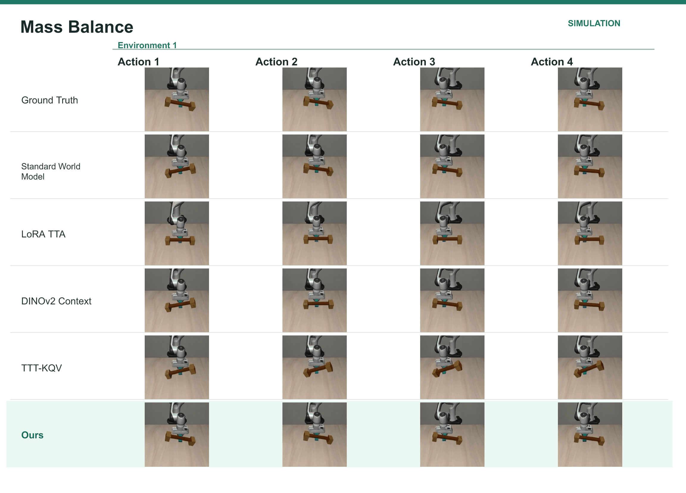
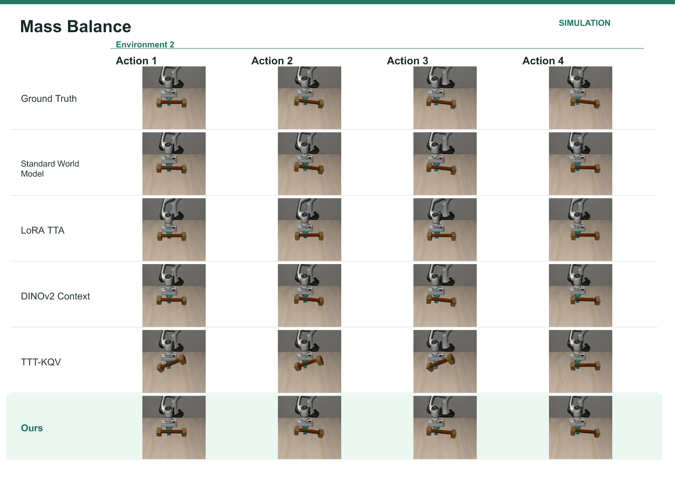
Across five single-factor tasks, action success rises from 36.9% to 76.6%. Friction mean error falls from 11.06 to 3.85 pixels, collision error from 21.93 to 6.45 pixels, and balance error from 1.18° to 0.64°. T2-z wins action success on these tasks but not every prediction metric: DINOv2 Context has lower gravity prediction errors and slightly better gravity appearance scores.
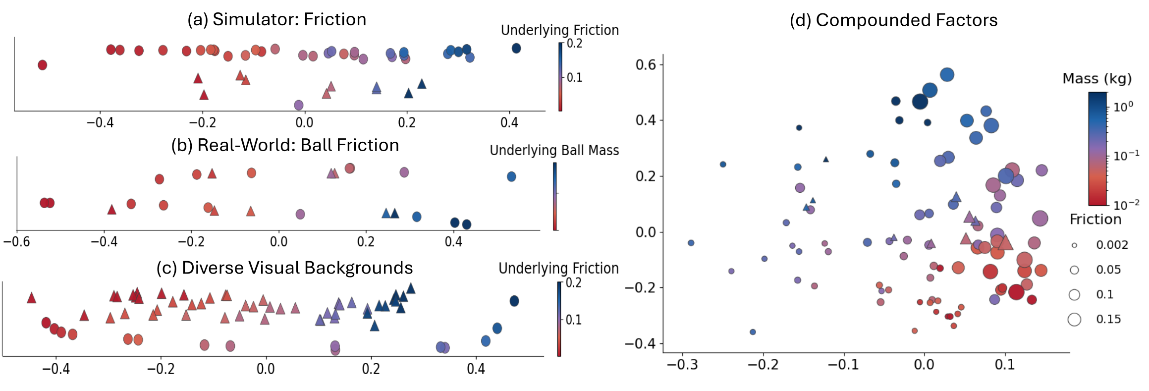
Emergent Structure of Environment Latents.
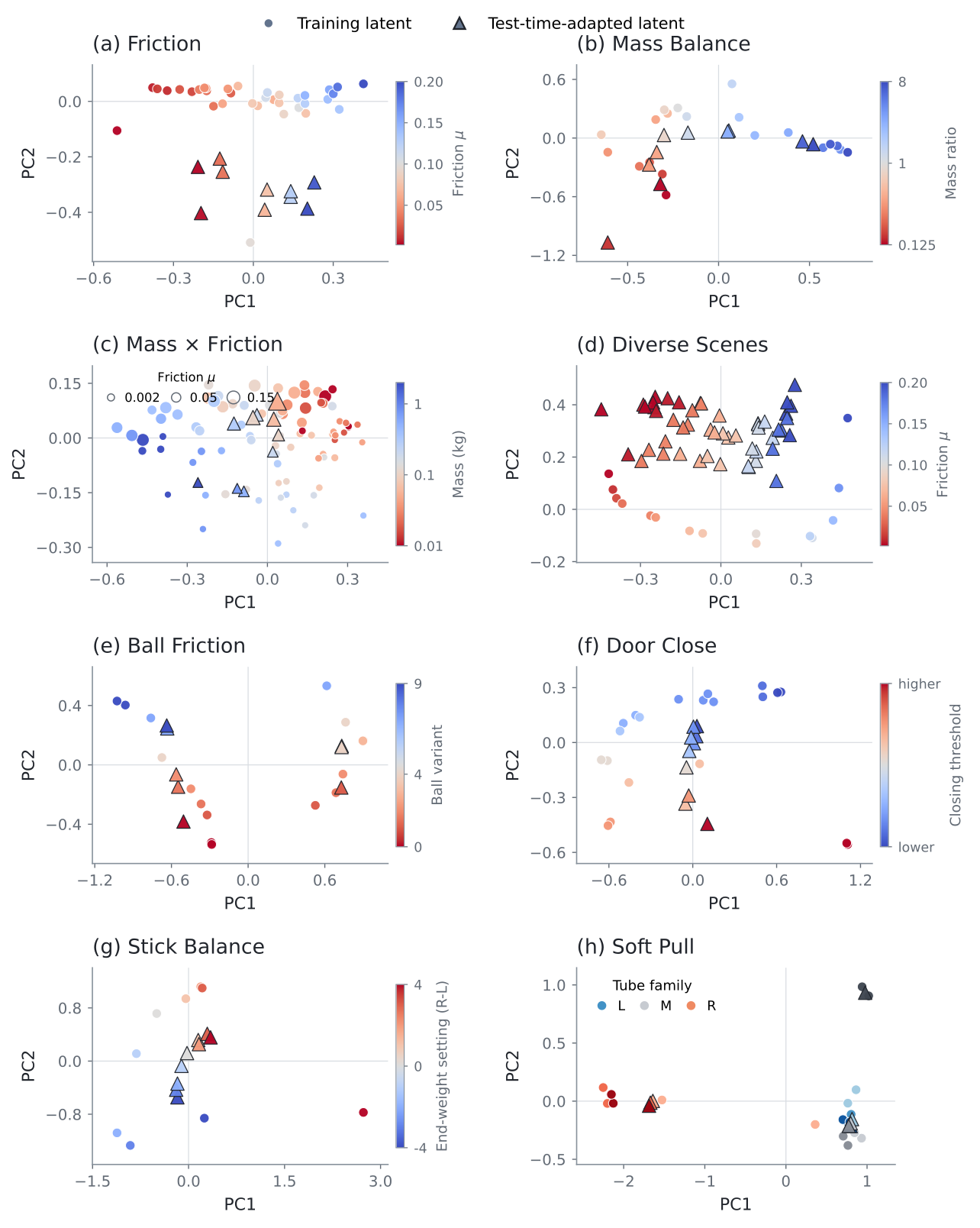
Two-dimensional PCA plots show organization correlated with held-out physical annotations. Those numerical factor values are used to interpret plots, not to train the vectors. Such projections support structured representations in these datasets; they do not establish uniquely identifiable physical coordinates or a general disentanglement theorem.
Compounded Environmental Factors.
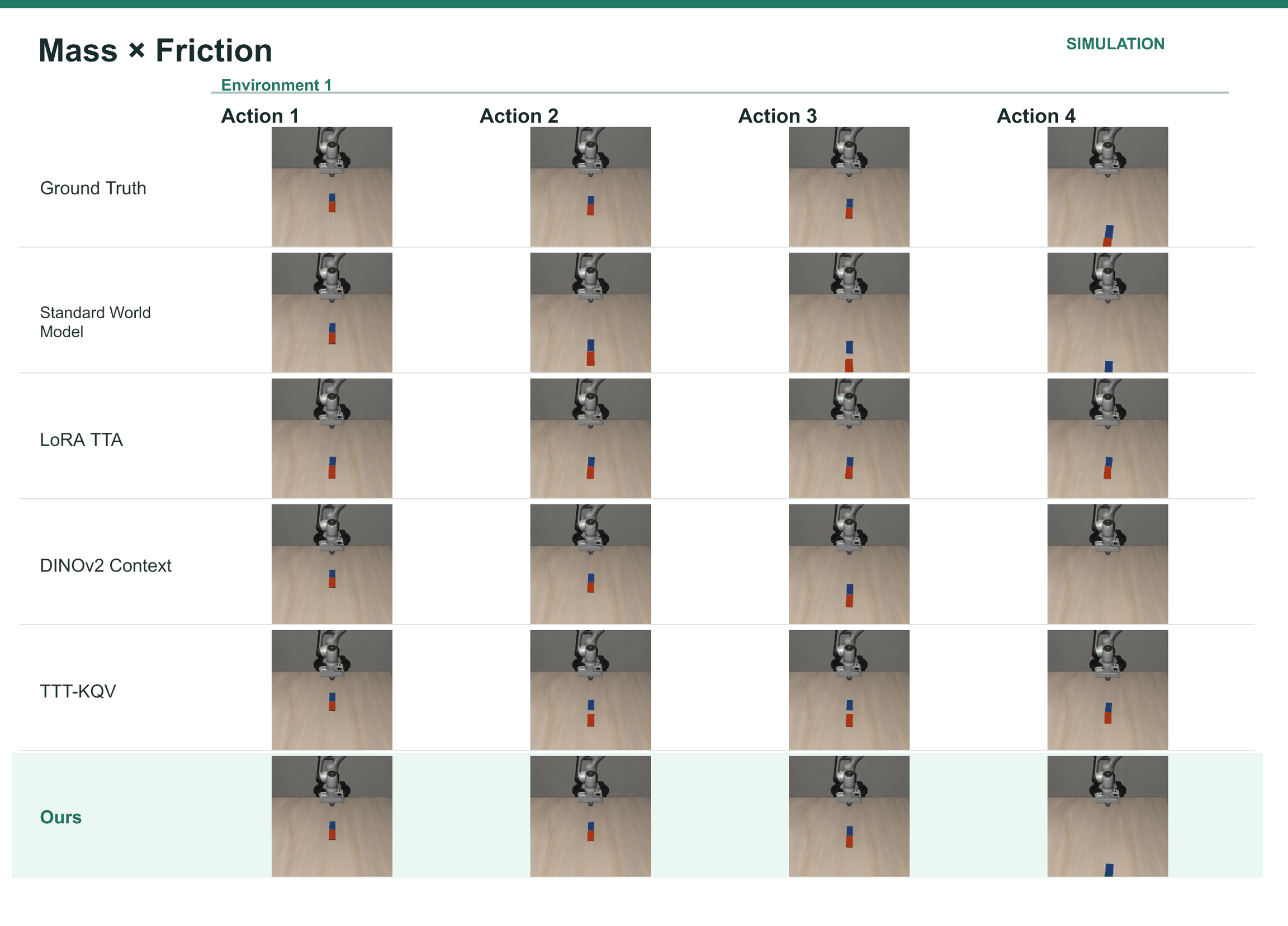
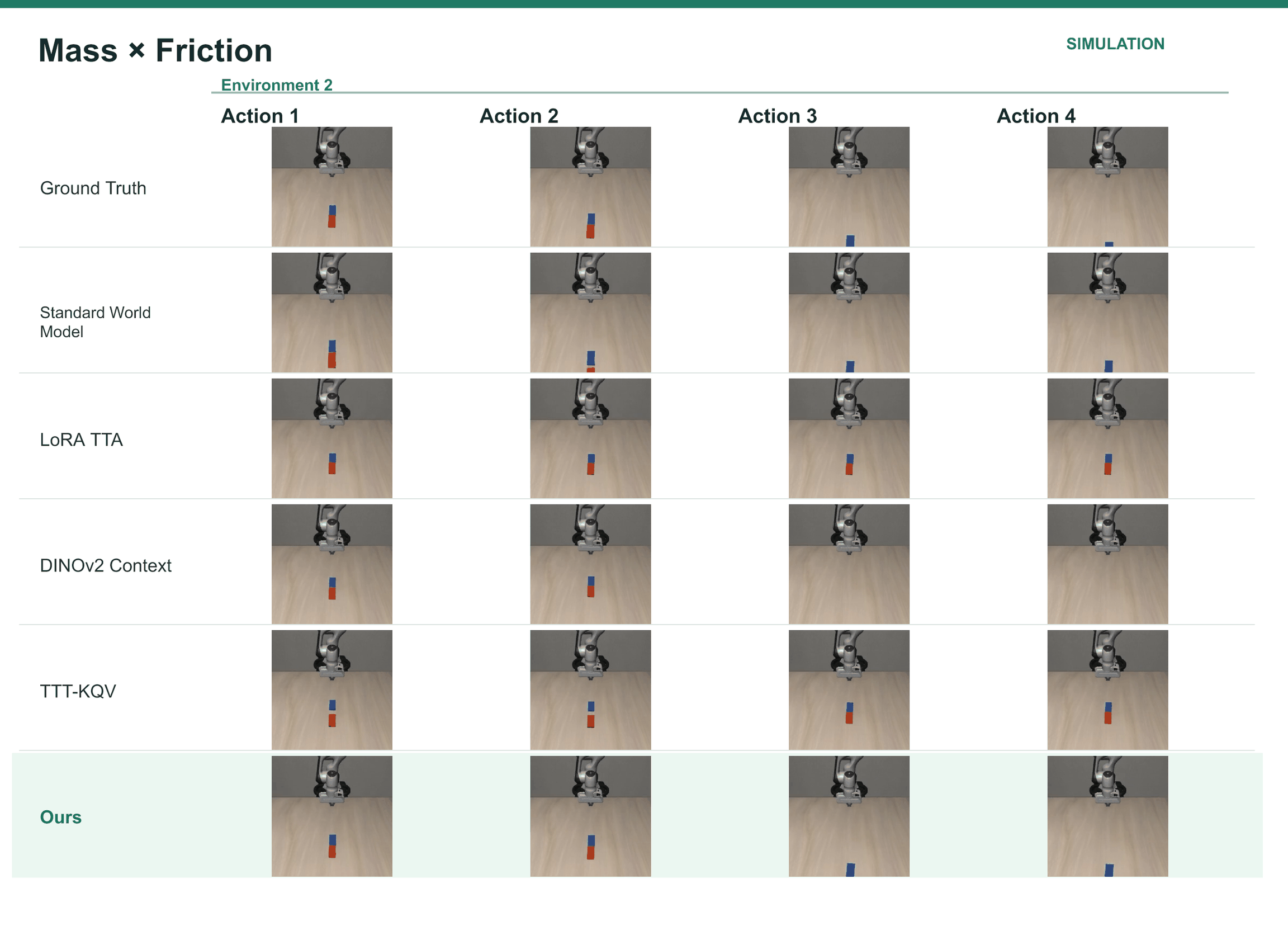
With mass and friction changing together, action success rises from 35.0% to 69.7% and positional errors improve. The plotted latent geometry correlates with both factors despite no numerical factor supervision. This demonstrates useful joint variation in the tested grid, not automatic recovery of every possible number or type of hidden factor.
Robustness across Diverse Visual Scenes.
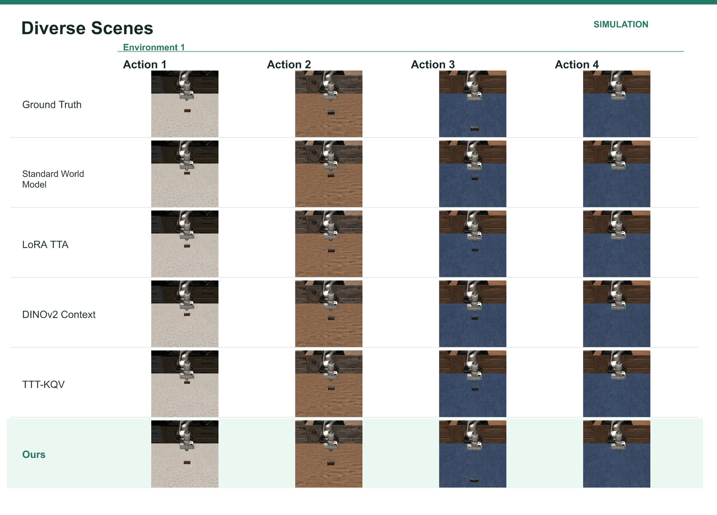
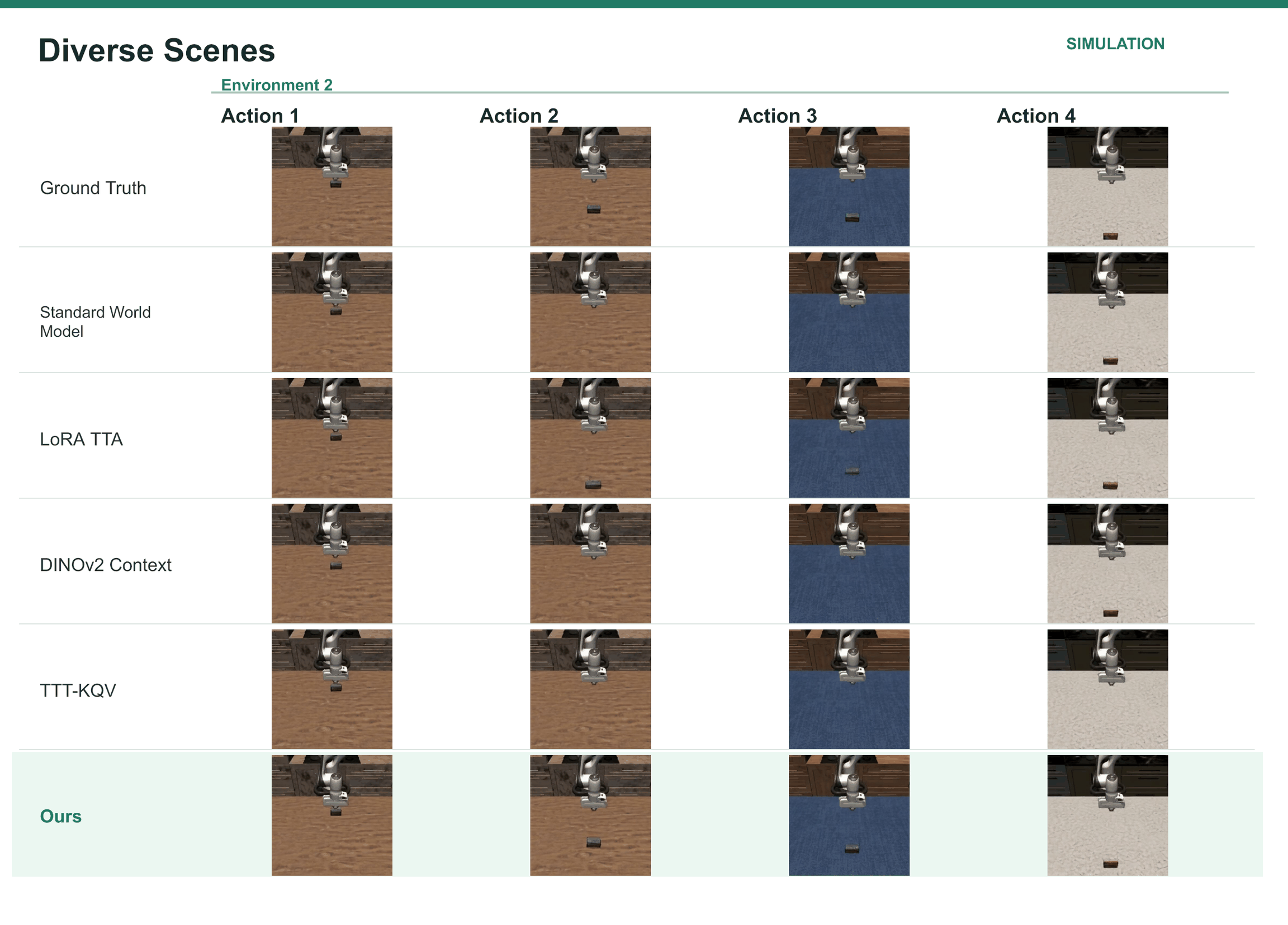
Across 30 visual backgrounds, T2-z reaches 66.7% success versus 45.8% without adaptation and improves all reported metrics. Similar friction settings organize together in the projected latent space. This is evidence of robustness to the evaluated backgrounds, rather than proof of complete appearance invariance.
| Task | Method | Physical Error (Mean) | Physical Error (Final) | LPIPS | PSNR | Action Success |
|---|---|---|---|---|---|---|
| Door Close | Standard World Model | 21.82 | 41.22 | 0.05700 | 29.96 | 22.22% |
| LoRA TTA | 17.35 | 32.14 | 0.04946 | 30.24 | 22.22% | |
| DINOv2 Context | 21.12 | 38.90 | 0.05490 | 30.28 | 22.22% | |
| TTT-KQV | 19.87 | 35.93 | 0.05164 | 30.95 | 22.22% | |
| T2-z (Ours) | 7.95 | 13.47 | 0.03208 | 32.15 | 55.56% | |
| Ball Friction | Standard World Model | 28.36 | 64.42 | 0.03153 | 36.04 | 0.00% |
| LoRA TTA | 37.48 | 72.09 | 0.03805 | 35.44 | 50.00% | |
| DINOv2 Context | 24.90 | 52.54 | 0.02934 | 36.32 | 12.50% | |
| TTT-KQV | 29.80 | 67.37 | 0.03224 | 36.29 | 25.00% | |
| T2-z (Ours) | 14.47 | 24.57 | 0.02401 | 36.23 | 62.50% | |
| Stick Balance | Standard World Model | 5.29 | 11.40 | 0.04716 | 31.87 | 20.00% |
| LoRA TTA | 3.63 | 7.24 | 0.04111 | 32.40 | 40.00% | |
| DINOv2 Context | 2.80 | 7.54 | 0.03640 | 33.58 | 20.00% | |
| TTT-KQV | 4.49 | 10.40 | 0.03948 | 33.38 | 25.00% | |
| T2-z (Ours) | 2.27 | 5.01 | 0.04175 | 32.05 | 83.33% | |
| Soft Pull | Standard World Model | 21.71 | 35.90 | 0.07207 | 33.32 | 63.64% |
| LoRA TTA | 18.63 | 26.20 | 0.06862 | 33.63 | 63.64% | |
| DINOv2 Context | 21.19 | 29.17 | 0.07087 | 33.47 | 72.73% | |
| TTT-KQV | 18.23 | 29.69 | 0.06439 | 34.03 | 72.73% | |
| T2-z (Ours) | 18.71 | 23.59 | 0.07580 | 32.52 | 81.82% | |
| Average | Standard World Model | 19.30 | 38.24 | 0.05194 | 32.80 | 26.47% |
| LoRA TTA | 19.27 | 34.42 | 0.04931 | 32.93 | 43.97% | |
| DINOv2 Context | 17.50 | 32.04 | 0.04788 | 33.41 | 31.86% | |
| TTT-KQV | 18.10 | 35.85 | 0.04694 | 33.66 | 36.24% | |
| T2-z (Ours) | 10.85 | 16.66 | 0.04341 | 33.24 | 70.80% |
4.3 Real-World Robotic Experiments
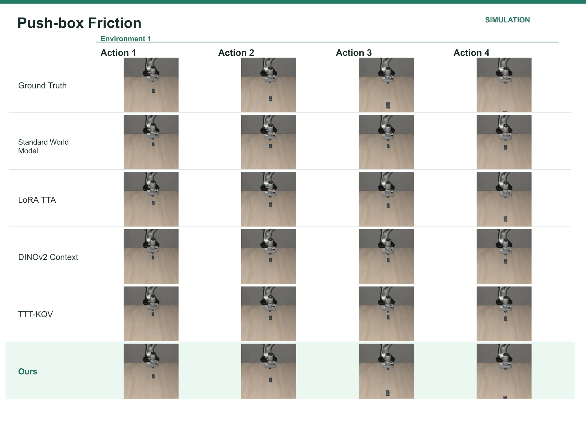
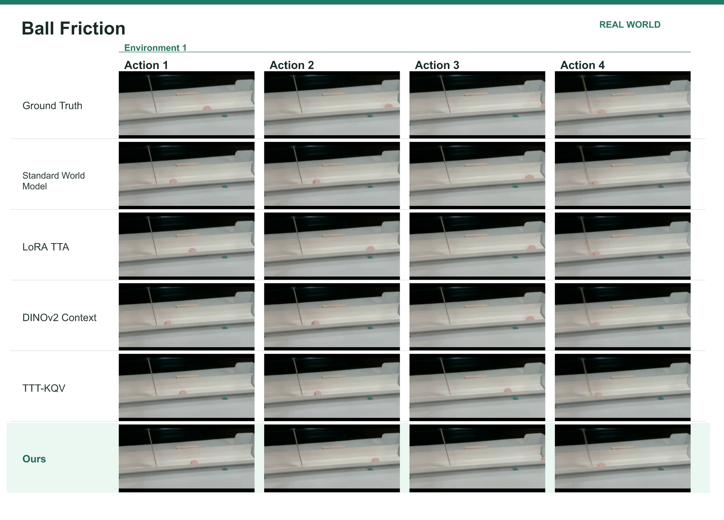
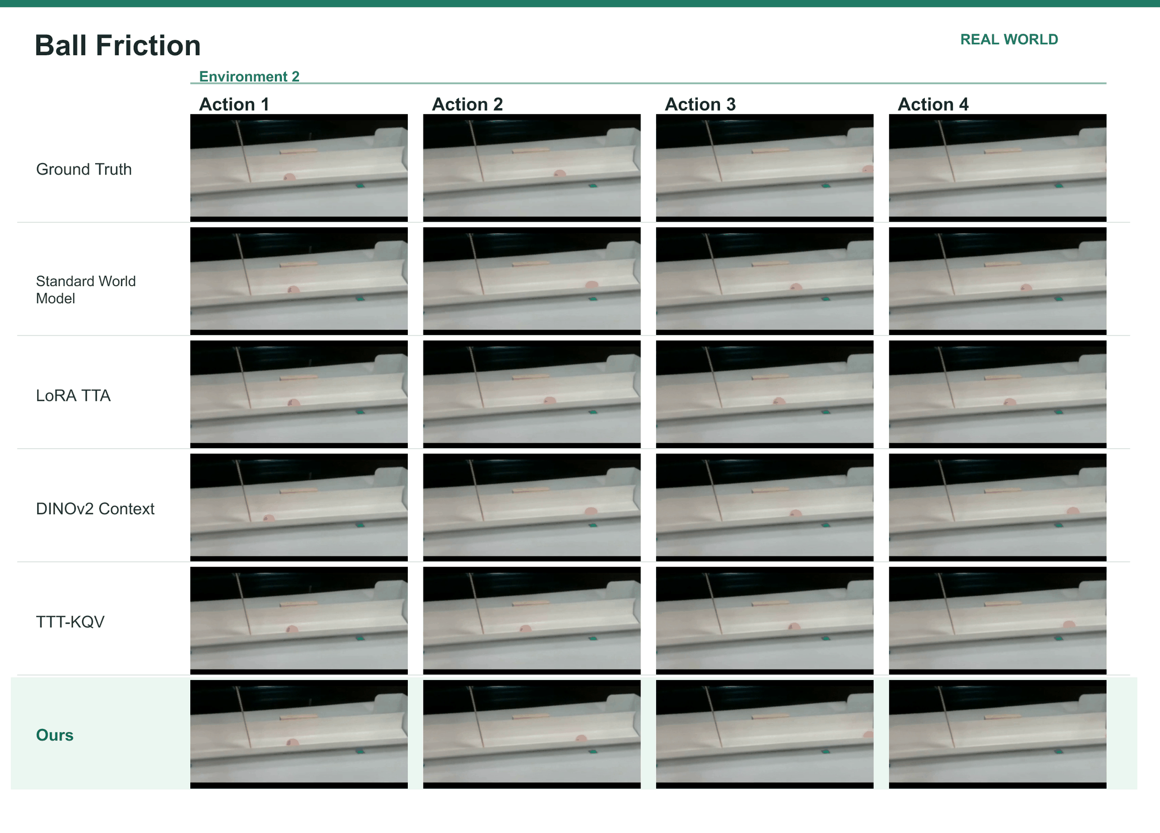
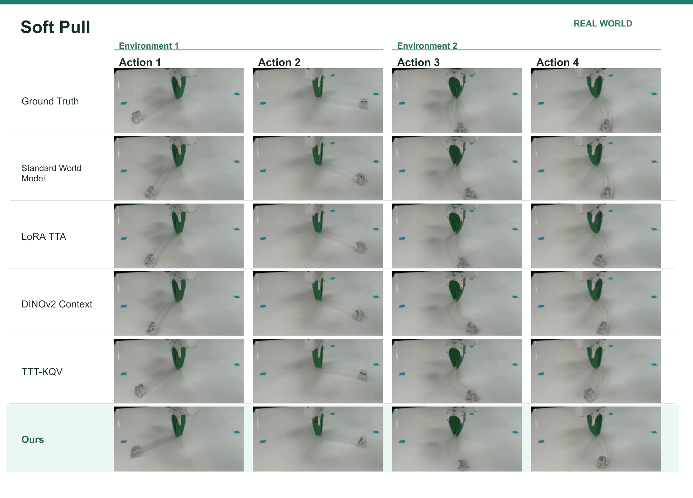
Hardware mean/final tracked-state error improves from 19.30/38.24 to 10.85/16.66 native-image pixels, and mean action success from 26.47% to 70.80%. Stick balance improves from 20.00% to 83.33%. T2-z does not win every appearance measure: its Soft Pull LPIPS is worse than all four baselines, and TTT-KQV has slightly lower Soft Pull mean positional error. Success protocols and native image scales differ across tasks.
4.4 Ablative & Qualitative Studies
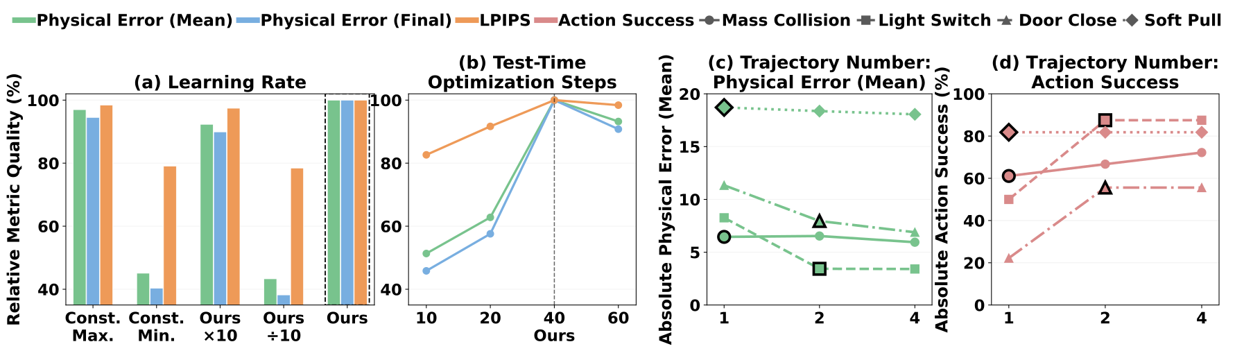
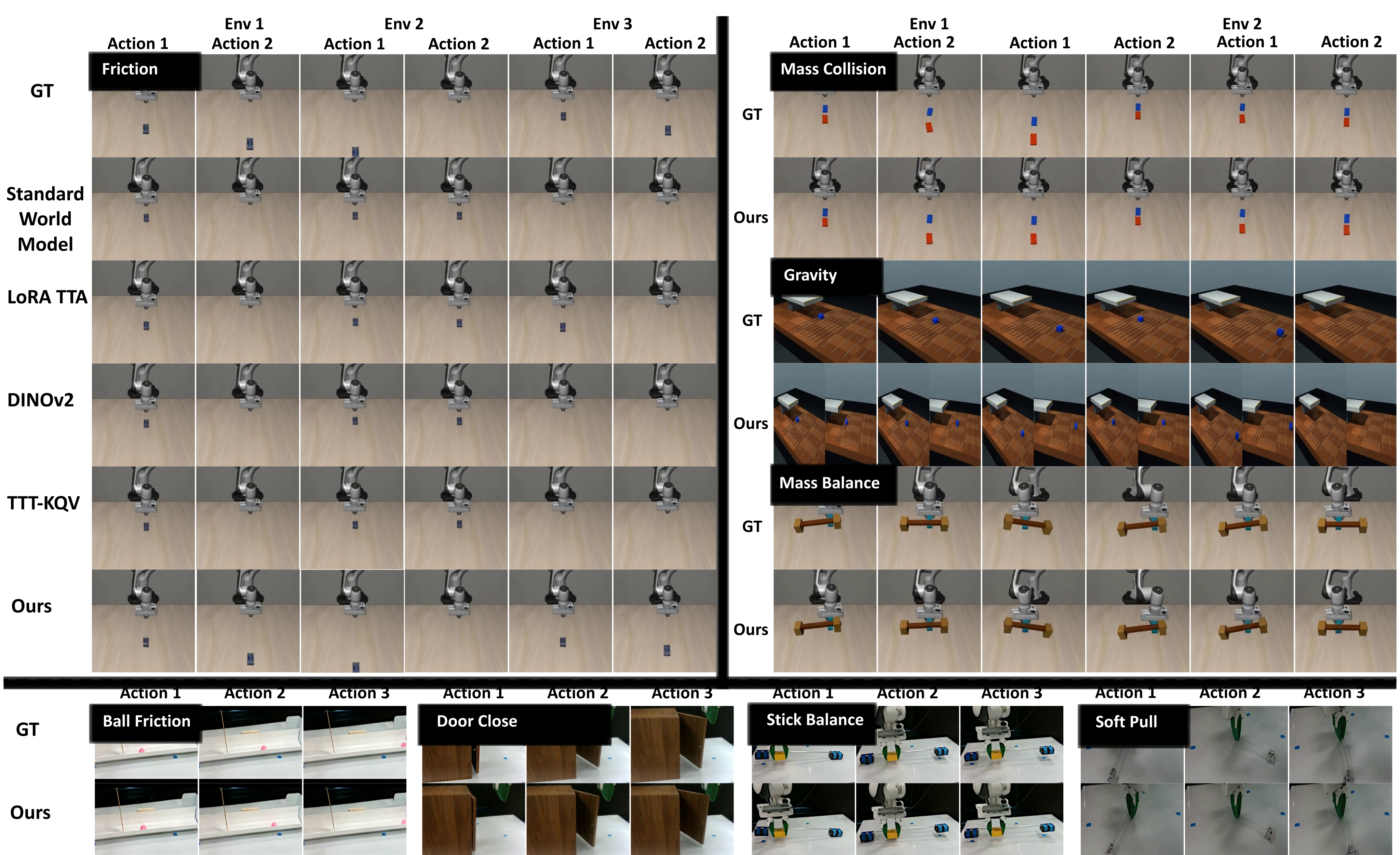
The selected coarse-to-fine schedule and 40-update budget outperform the tested alternatives. Joint training, a directly optimized 3072-D token, another initialization range and shorter/longer alternation blocks generally weaken Friction results, although some appearance scores improve. Interaction counts have task-dependent effects; the collision success rate continues from 61.1% at one trajectory to 72.2% at four. Selected visual examples complement, rather than replace, quantitative results.
| Method | Physical Error (Mean) | Physical Error (Final) | LPIPS | PSNR | Action Success |
|---|---|---|---|---|---|
| Joint Model-Latent Training | 7.03 | 15.66 | 0.0657 | 31.203 | 68% |
| Direct Token (3072-D) | 94.50 | 80.49 | 0.7626 | 15.218 | 24% |
| 32-D Random | 4.81 | 9.73 | 0.0495 | 32.172 | 60% |
| Alternating Latent/Model (100/100) | 5.41 | 11.50 | 0.0484 | 32.208 | 56% |
| Alternating Latent/Model (400/400) | 4.31 | 8.80 | 0.0507 | 32.430 | 68% |
| T2-z | 3.85 | 7.59 | 0.0495 | 31.976 | 72% |
5 Conclusion
A small optimized environment vector can adapt a frozen world model and improve action selection in these controlled settings. The paper has no separate limitations section. Practical boundaries include environment-grouped training, observed adaptation interactions, expensive shared video generation, task-specific training and evaluation, and candidate sets known to contain a feasible action. Latent plots and few-interaction results do not guarantee recovery of unobserved factors in general.
Acknowledgements
Funding acknowledgements credit ONR MURI programs, Singapore MDDI, the Korean IITP/MSIT program, 2077AI and Toyota Research Institute’s university program.
Contents
The supplement covers model conditioning and optimization, dataset budgets, exact evaluation protocols, baseline implementations, ablations, compute profiling and all selected qualitative comparisons.
Appendix A Model Architecture and Optimization
Implementation details specify which components learn during each phase and where the environment vector enters the inherited architecture.
A.1 Architecture and latent conditioning
One initial RGB frame and an aligned 14-D action sequence condition future video prediction. The environment vector enters both attention and timestep modulation.
Inputs and inherited backbone.
BWM supplies the pretrained video transformer and action encoder; the Wan video autoencoder stays frozen. Text conditioning is disabled. The initial image enters the video-latent stream, rather than becoming an extra cross-attention token.
Environment-indexed latent conditioning.
Episodes in one environment share a free 32-D vector. Separate bias-free 32→128→3072 projectors, each with normalization and GELU, create attention and modulation representations. The 128-D size is an internal hidden width, not the final conditioning dimension.
Equation 9
| (9) | ||||
Cross-attention branch.
One projected environment token is prepended to encoded action tokens. Every video patch can attend to both through cross-attention keys and values. The displayed equation is a schematic attention head; implementation is multi-head.
Equation 10
| (10) |
Modulation branch.
Groups of four actions map to modulation vectors for aligned video-latent time groups. These add to the noise-timestep embedding and projected environment vector before the inherited time projection. Six width-3072 outputs control normalization shifts/scales and residual gates; the modified timestep embedding also conditions the output head.
Equation 11
| (11) |
| Component | Initialization or structure | Training update |
|---|---|---|
| Video DiT | BWM-initialized Wan2.2 backbone | Model blocks |
| Action encoder | BWM-initialized 14-D action pathway | Model blocks |
| Video VAE | Wan2.2 video encoder/decoder | Frozen |
| Environment table | Learnable 32-D latents indexed by environment | Latent blocks |
| Latent projectors | Two MLPs | Model blocks |
A.2 Training and test-time adaptation
Training alternates shared-weight and environment-table optimization. Deployment keeps all shared components, including the two projectors, fixed.
Training schedule.
The loss excludes the initial conditioning frame. Model blocks update the transformer, action encoder and latent projectors using AdamW at 10⁻⁵, weight decay 0.01, 100 warmup updates, clipping 0.5 and bfloat16. Latent blocks use learning rate 0.03 with zero weight decay; uniformly initialized training latents are clipped to [0,1] after updates.
Test-time adaptation.
A fresh 32-D vector is fit for each held-out environment using 40 updates and the four-stage schedule. Its interaction videos are distinct from query outcomes. The same fitted vector is reused across that environment’s query actions; task-specific execution configurations are referred to the released code.
Appendix B Experimental Setup
Tables 5–6 retain task-level data counts, frame/chunk settings, batch structure, image resolutions and compute budgets.
B.1 Training data and resource budgets
Counts are physical environments and recorded episodes, not latent entries. Simulation ranges from 12 to 84 environments; hardware uses 8–10 environments and 146–438 episodes per task. Typical training budgets are two H200 GPUs for 24 hours per method; joint mass/friction uses four for 48 hours and diverse backgrounds four for 24. Batch notation is environments × chunks per environment. These are task-level models and budgets, not one jointly trained eleven-task model.
| Task | Physical envs. episodes/env. | Frames | Stride | Batch | Budget |
|---|---|---|---|---|---|
| Friction | 41 | 1 | |||
| Gravity | 61 | 1 | |||
| Mass Collision | 61 | 1 | |||
| Light Switch | 33 | 1 | |||
| Mass Balance | 41 | 2 | |||
| Mass Friction | 61 | 1 | |||
| Diverse Backgrounds | 41 | 1 |
| Task | Physical envs. / episodes | Frames | Stride | Native RGB | Input RGB | Batch | Budget |
|---|---|---|---|---|---|---|---|
| Ball Friction | 8 / 240 | 61 | 1 | ||||
| Door Close | 10 / 438 | 49 | 1 | ||||
| Stick Balance | 9 / 421 | 33 | 3 | ||||
| Soft Pull | 9 / 146 | 33 | 3 |
B.2 Simulator and real-world setup
Simulation and hardware use Franka arms and 14-channel action representations, with task-dependent target-action meaning.
Simulator.
Custom tasks run in a LIBERO-based simulator with a Franka Panda, 224×224 RGB frames and 20 Hz recording. Figure 7 retains representative views and tracked targets.
Real world.
Hardware uses a fixed RealSense D435i main RGB view at 640×480 and 20 Hz. Task-dependent crops are letterboxed to the model-input sizes in Table 6. Native-image pixel errors therefore should not be read as metric distances or as resolution-normalized scores.
Appendix C Evaluation Protocols
These protocols define what is observed during adaptation, what is predicted at query time, and how actual action success is judged.
C.1 Shared protocol and metrics
Prediction and action selection use shared queries across methods. Tables 7 and 9 report query-video counts, which are not automatically the numbers of action-selection trials.
Shared comparison.
Every evaluated candidate-action set contains at least one successful option; none of its query outcomes is exposed before prediction. Position error averages tracked-point distances or uses the final frame; scalar tasks use their own units. LPIPS uses unmasked full-frame AlexNet features, averaged over future frames then query videos. PSNR/SSIM also measure appearance. Interaction count K is per test environment, while query counts sum across environments.
Equation 12
| (12) |
| Task | Query videos | |
|---|---|---|
| Friction | 1 | 90 |
| Gravity | 1 | 90 |
| Mass Collision | 1 | 80 |
| Light Switch | 2 | 60 |
| Mass Balance | 2 | 130 |
| Mass Friction | 1 | 80 |
| Diverse Backgrounds | 1 | 90 |
C.2 Simulated tasks
Seven simulated settings vary hidden dynamics or rules while evaluating task-relevant outcomes. Main query counts range from 60 to 130 video chunks per setting.
| Task | Tracked quantity | Object-centric error |
|---|---|---|
| Friction | Pushed-block centroid | ADE/FDE |
| Gravity | Blue projectile centroid | ADE/FDE |
| Mass Collision | Red struck-object centroid | ADE/FDE |
| Light Switch | Yellow-pixel fraction in lamp region | Mean/final absolute error (pp) |
| Mass Balance | Balance-bar tilt angle | Mean/final angle error (∘) |
| Mass Friction | Red struck-object centroid | ADE/FDE |
| Diverse Backgrounds | Pushed-block centroid | ADE/FDE |
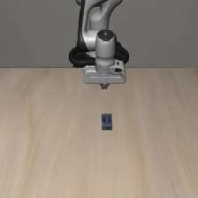
(a) Friction
(b) Gravity
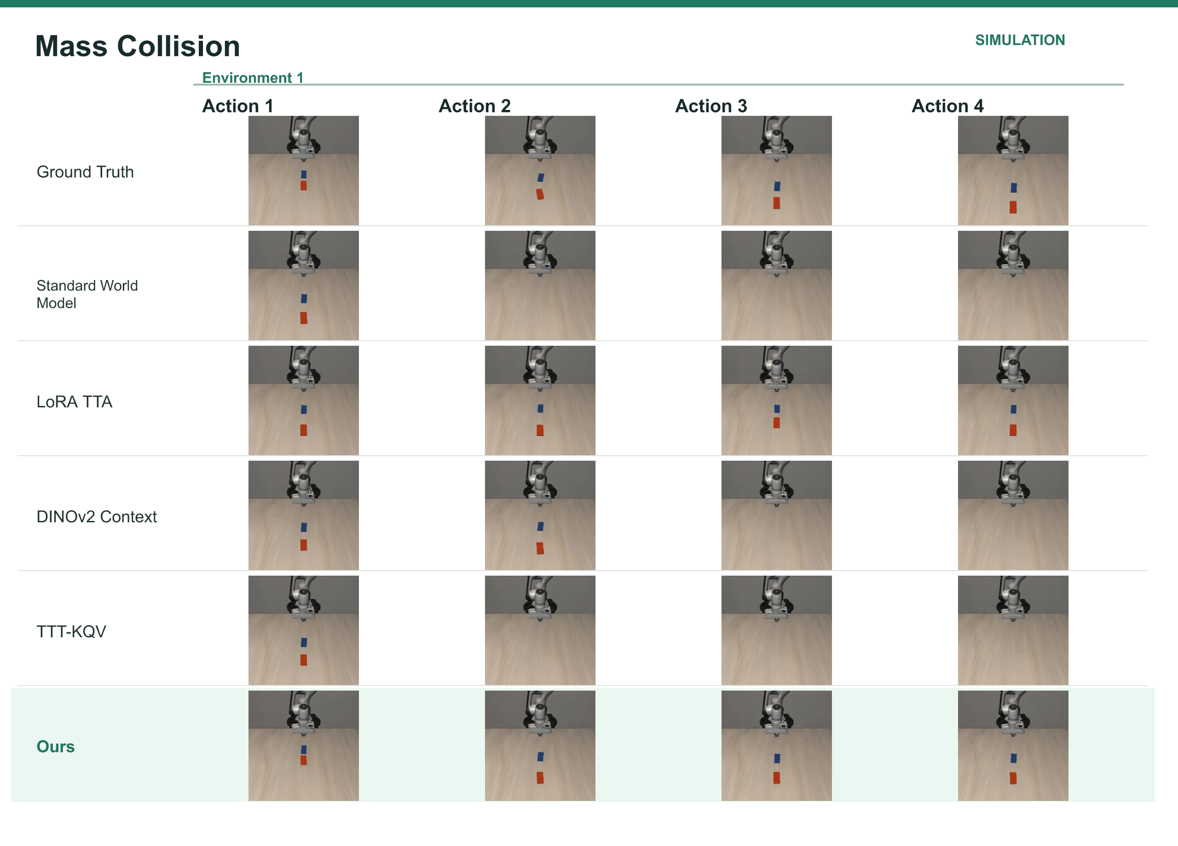
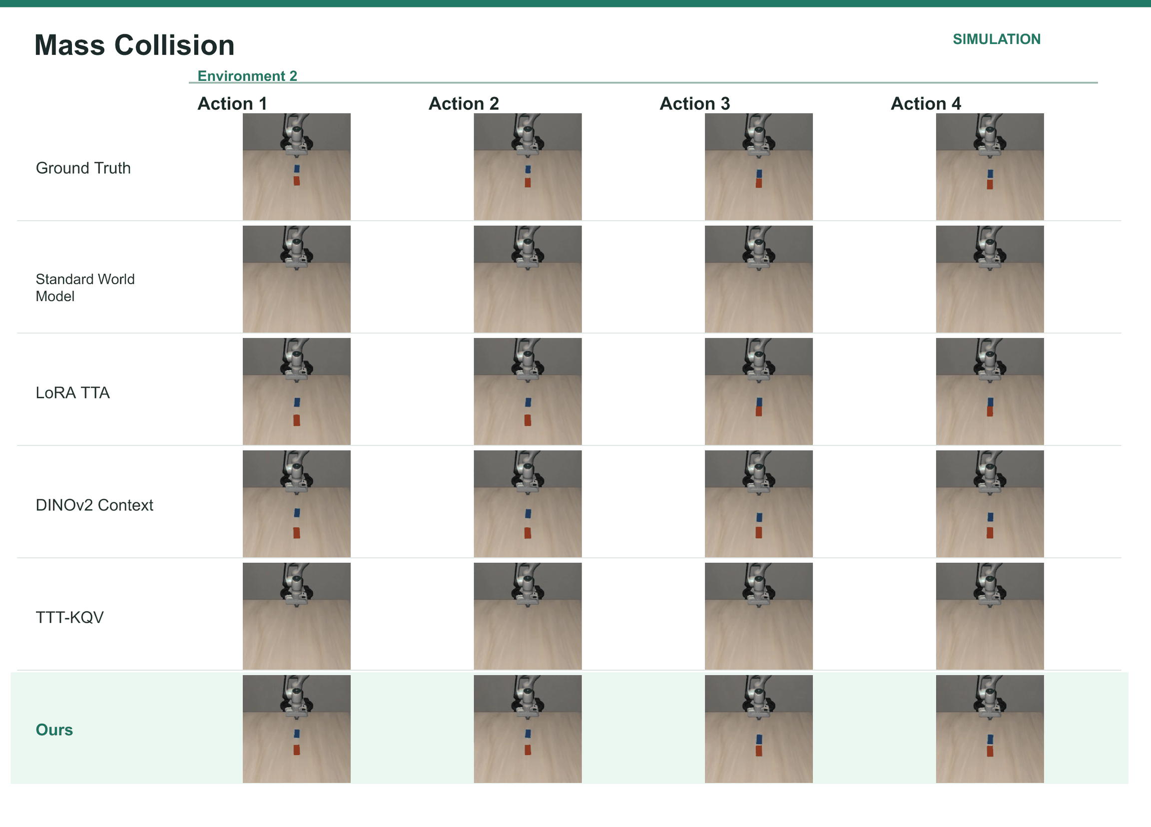
(c) Mass Collision
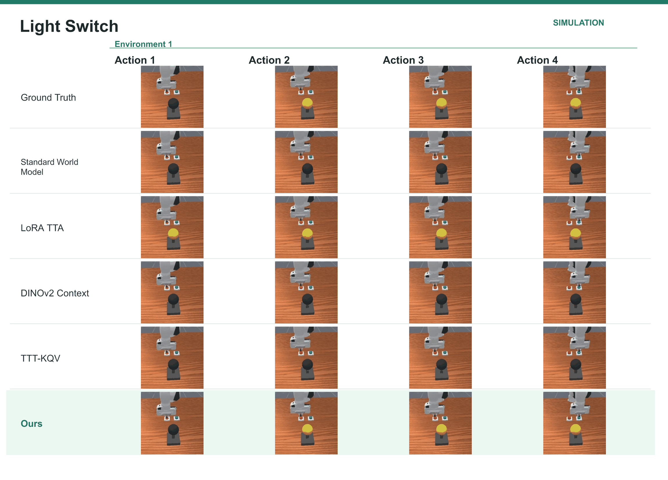
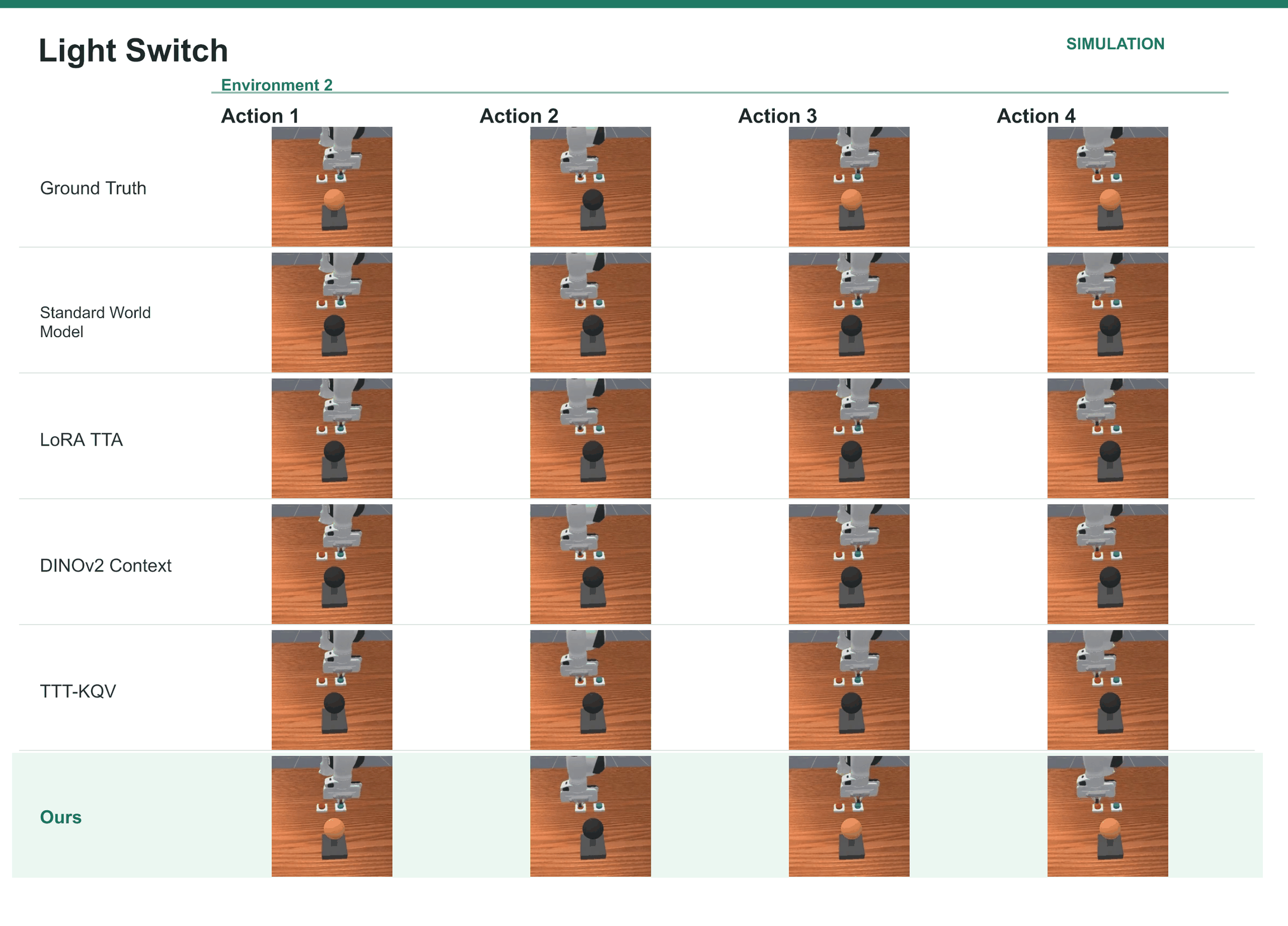
(d) Light Switch
(e) Mass Balance
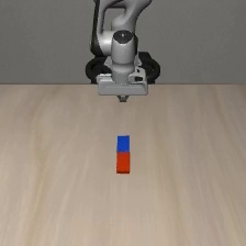
(f) Mass Friction
Friction.
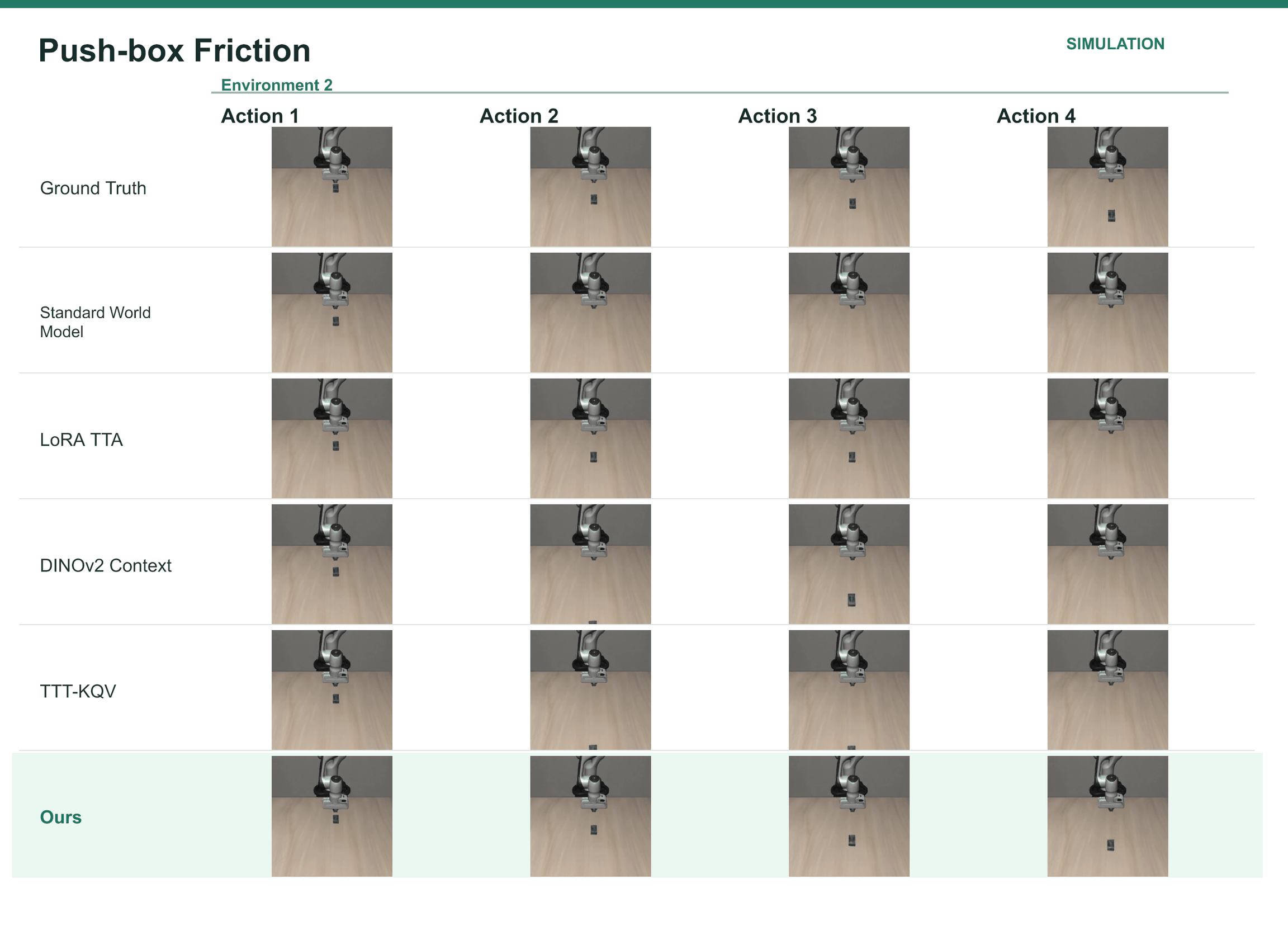
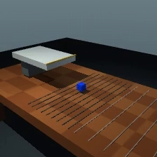
Vary table friction and push strength; track the pushed block’s centroid. Success requires observed displacement in the requested short, medium or long region.
Gravity.
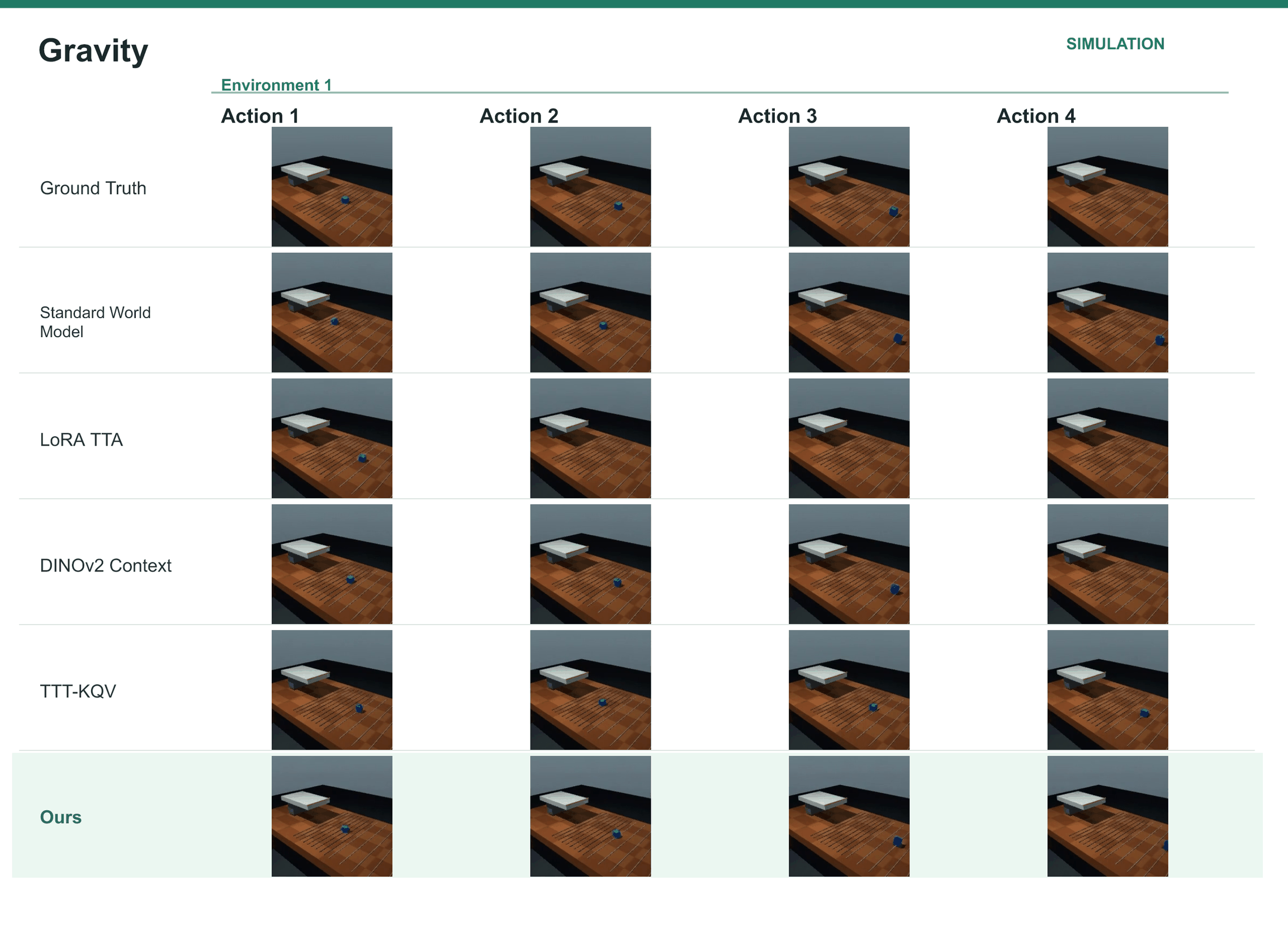
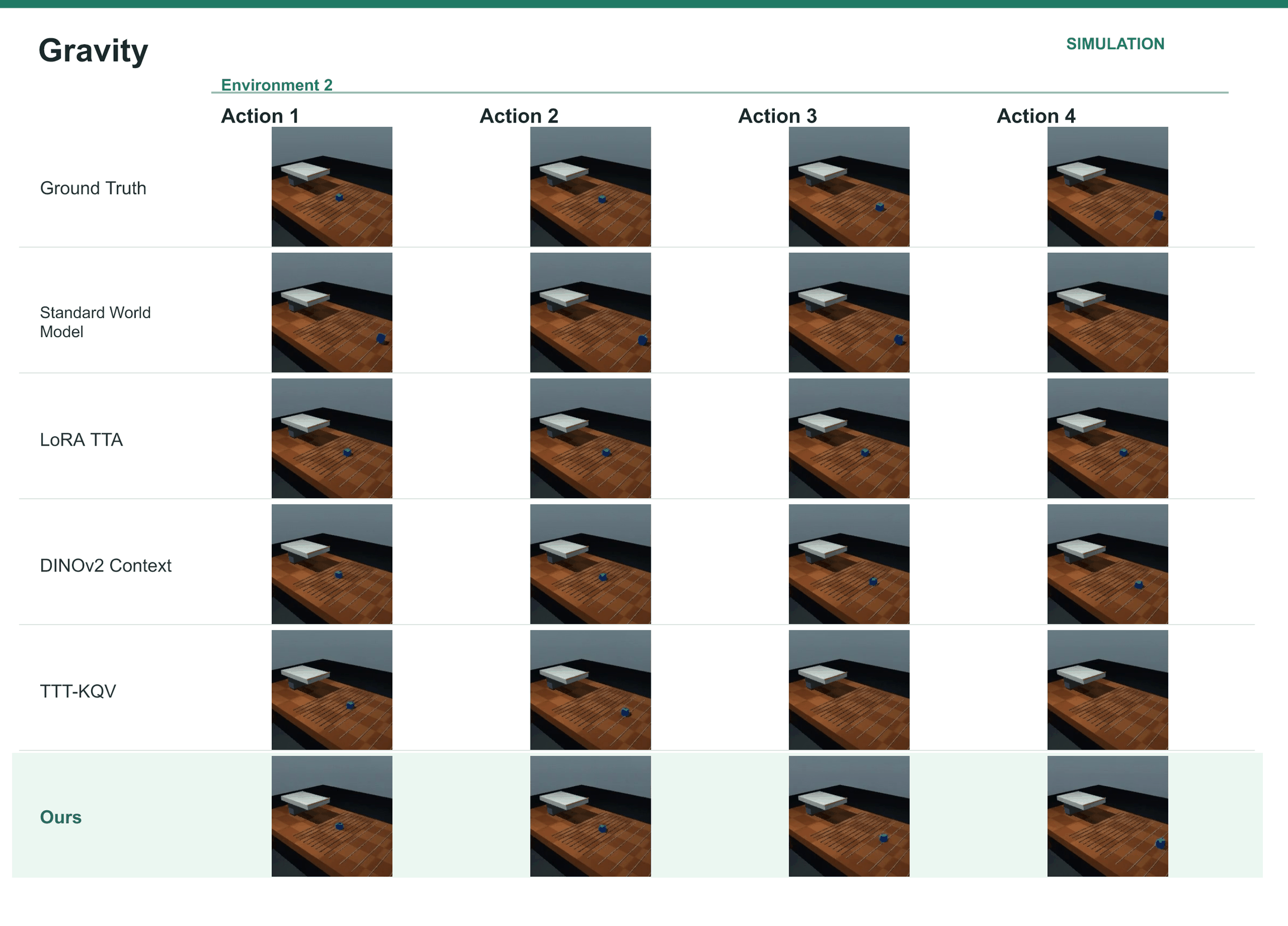
Vary gravity and projectile launch speed. Track the blue block and judge whether its observed endpoint reaches the requested near, middle or far region.
Mass Collision.
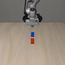
Vary the struck red object’s mass while a driver object collides with it. Track the red target rather than the driver and judge its displacement region.
Light Switch.
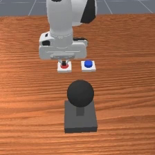
Hidden rules determine whether red, blue, both or neither button changes the lamp. A fixed RGB rule measures yellow-pixel fraction inside the lamp region; errors are percentage-point differences, not average-brightness errors. A score of at least 0.35 means on, and success matches the requested terminal on/off state.
Equations 13–14
| (13) |
| (14) |
Mass Balance.
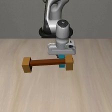
Vary left/right mass ratio while changing the robot support position as the action. Track bar angle in degrees; success means the final angle falls in the horizontal-balance interval.
Mass × Friction.
Vary collision mass and surface friction jointly. Track the struck red object; select the least forceful sampled action whose predicted endpoint crosses a target line, then evaluate the observed outcome.
Diverse Backgrounds (multi-background).
Repeat the friction push task across varied backgrounds. Background changes appearance rather than the action definition; centroid displacement remains the outcome and target.
C.3 Real-world tests
Hardware evaluates 80 ball, 100 door, 45 stick and 24 tube query videos. Ball/tube adaptation uses one interaction; door/stick use two. These query counts differ from action-success denominators.
| Task | Query videos | |
|---|---|---|
| Ball Friction | 1 | 80 |
| Door Close | 2 | 100 |
| Stick Balance | 2 | 45 |
| Soft Pull | 1 | 24 |
| Task | Tracked quantity | Object-centric error |
|---|---|---|
| Ball Friction | Visible ball center | ADE/FDE |
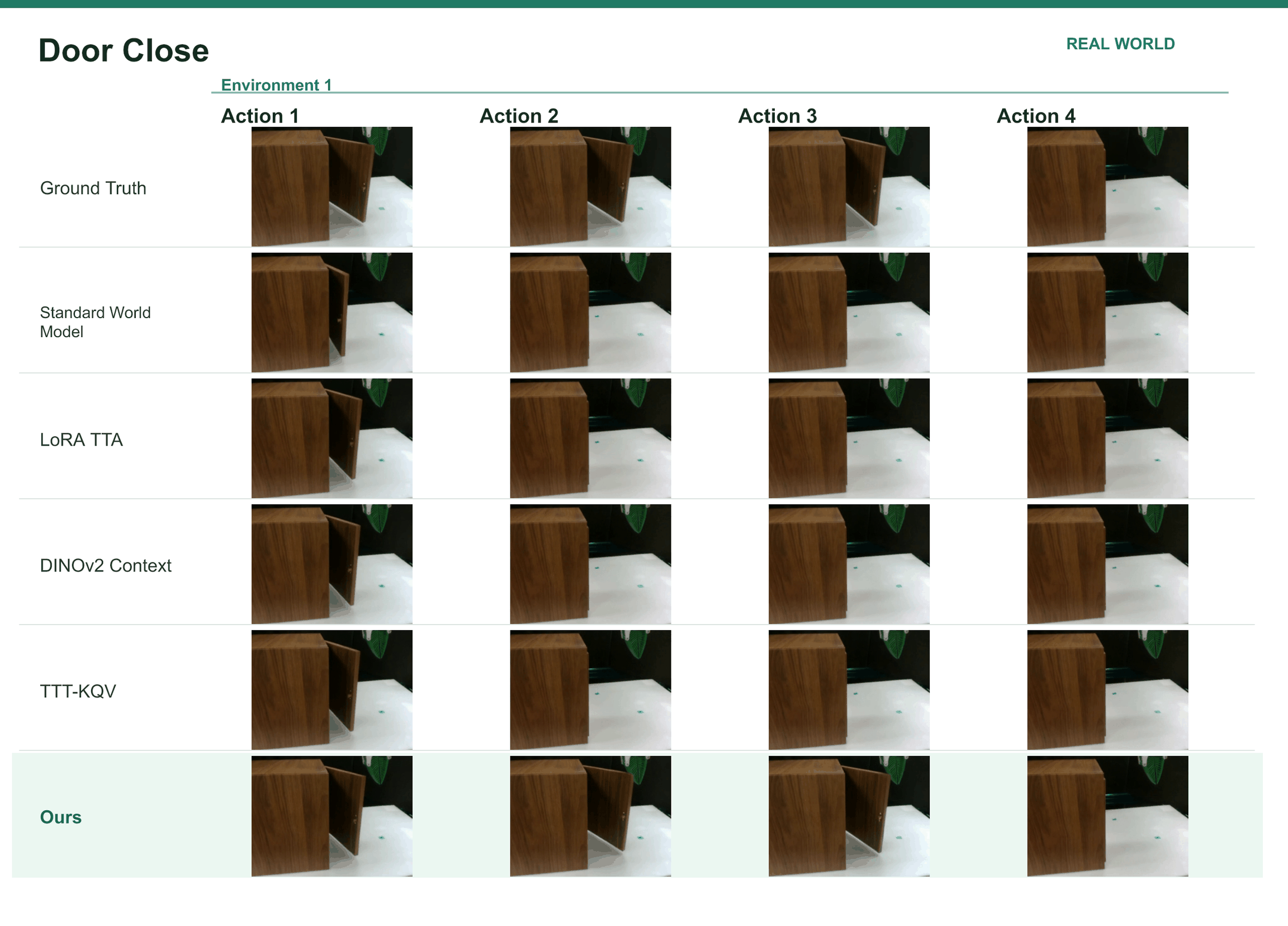
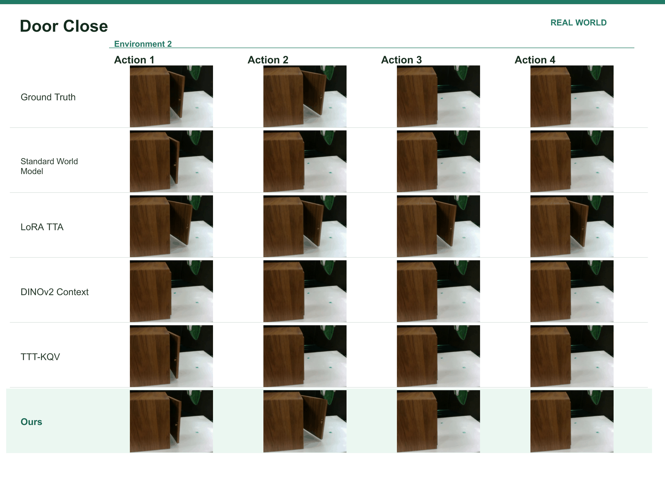
| Door Close | Outer door-edge position | ADE/FDE |
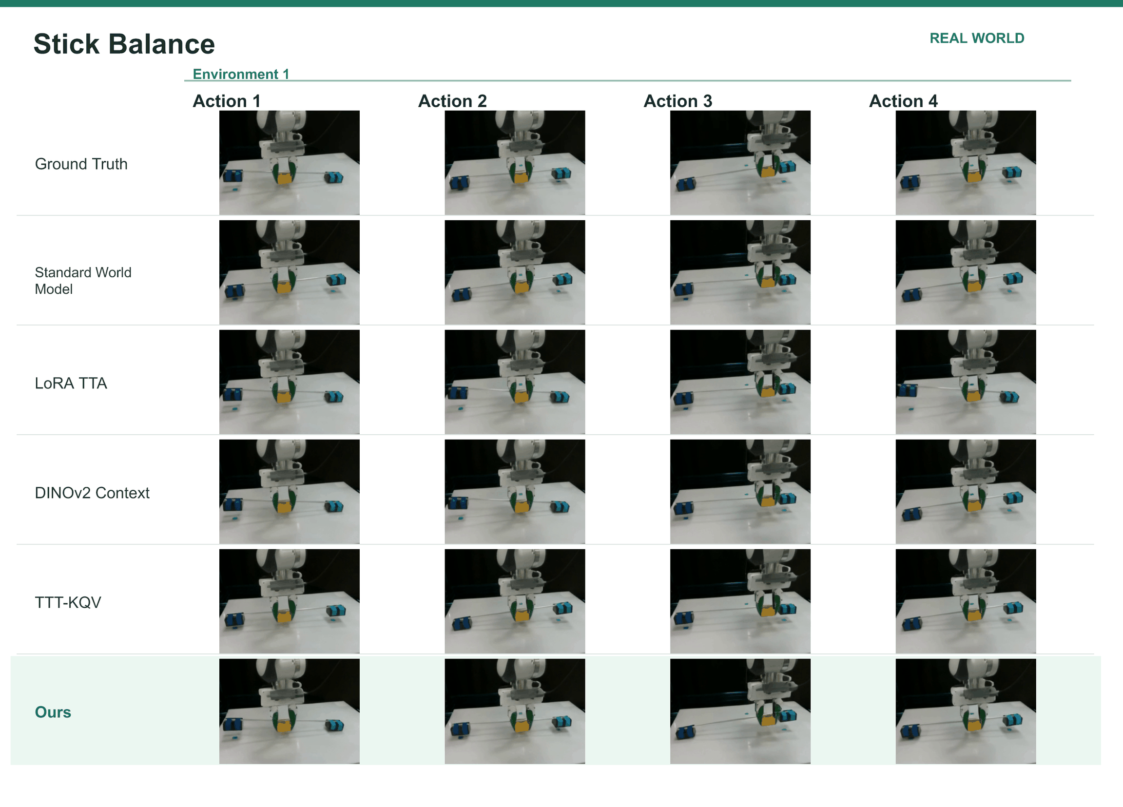
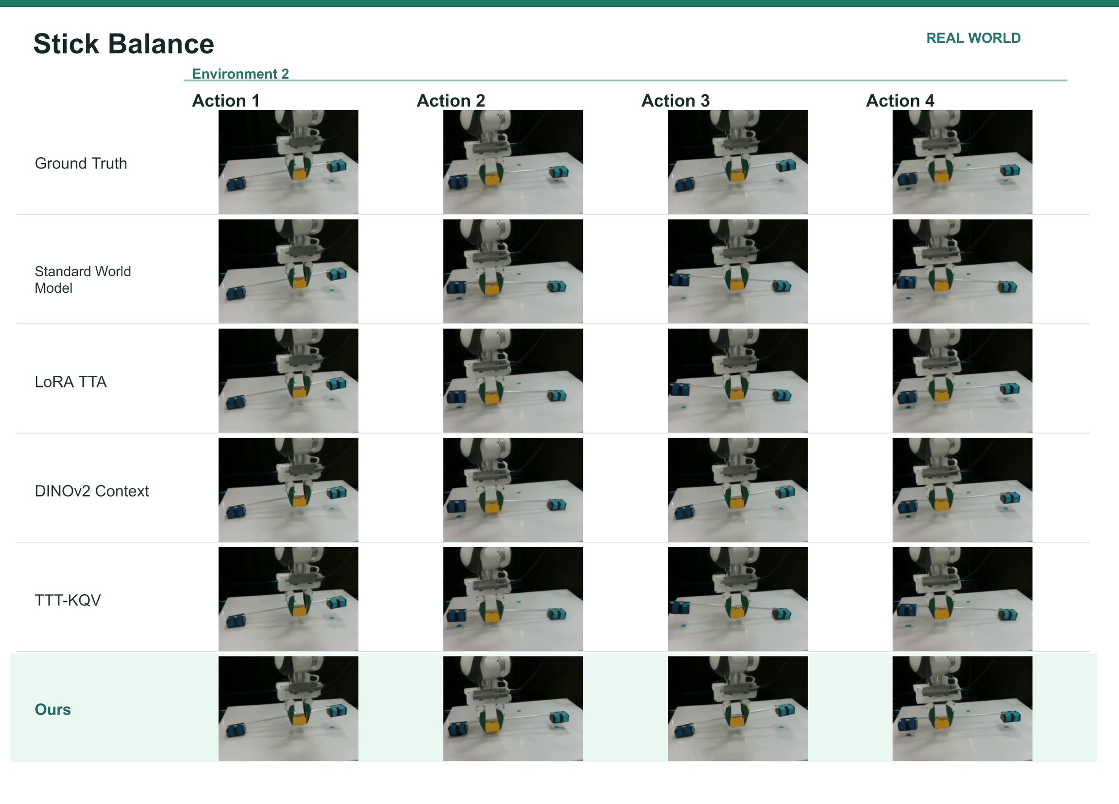
| Stick Balance | Two end markers, averaged | ADE/FDE |
| Soft Pull | Dragged object’s visible center | ADE/FDE |
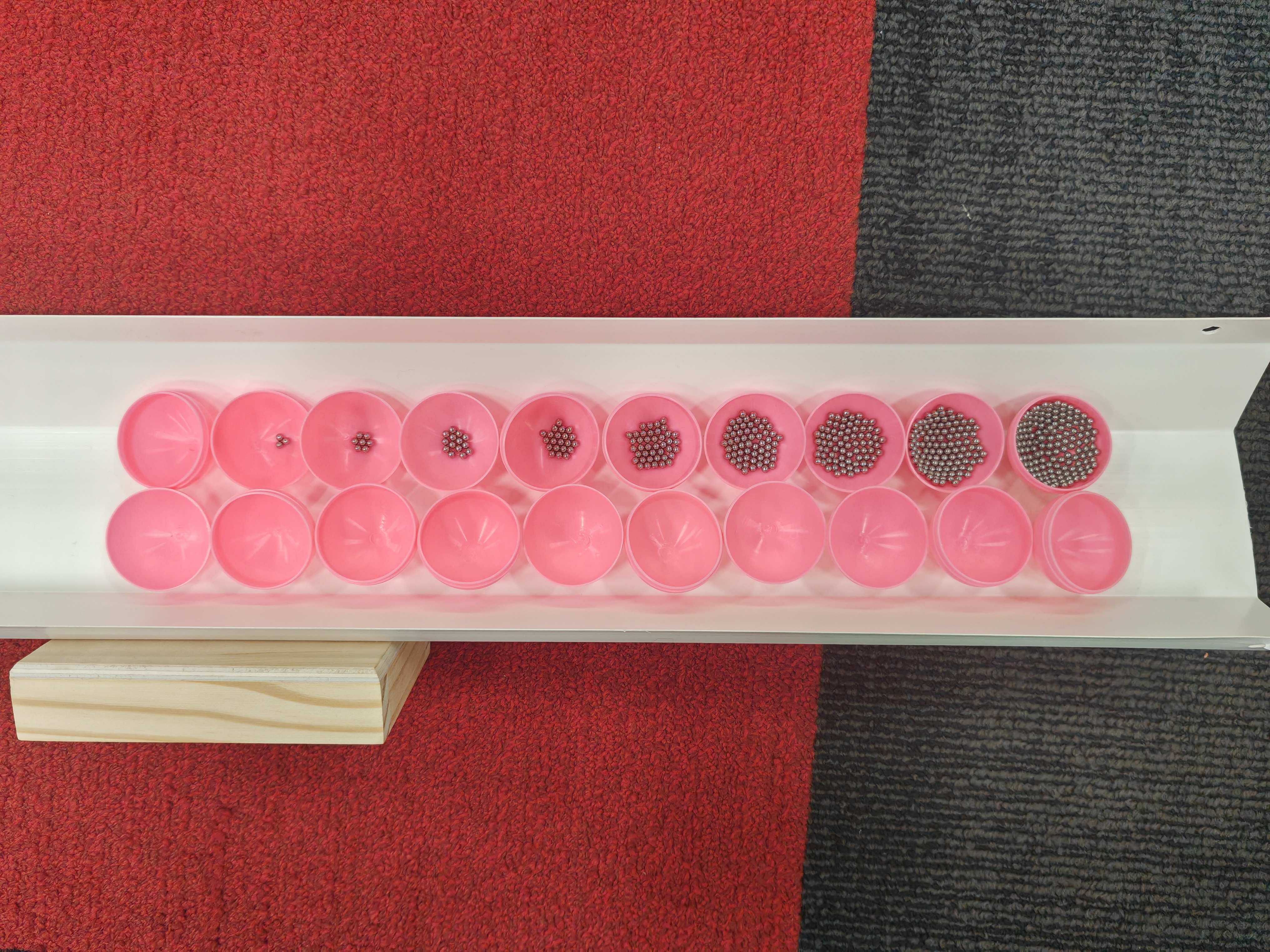
(a) Steel-bead loads for the ball variants
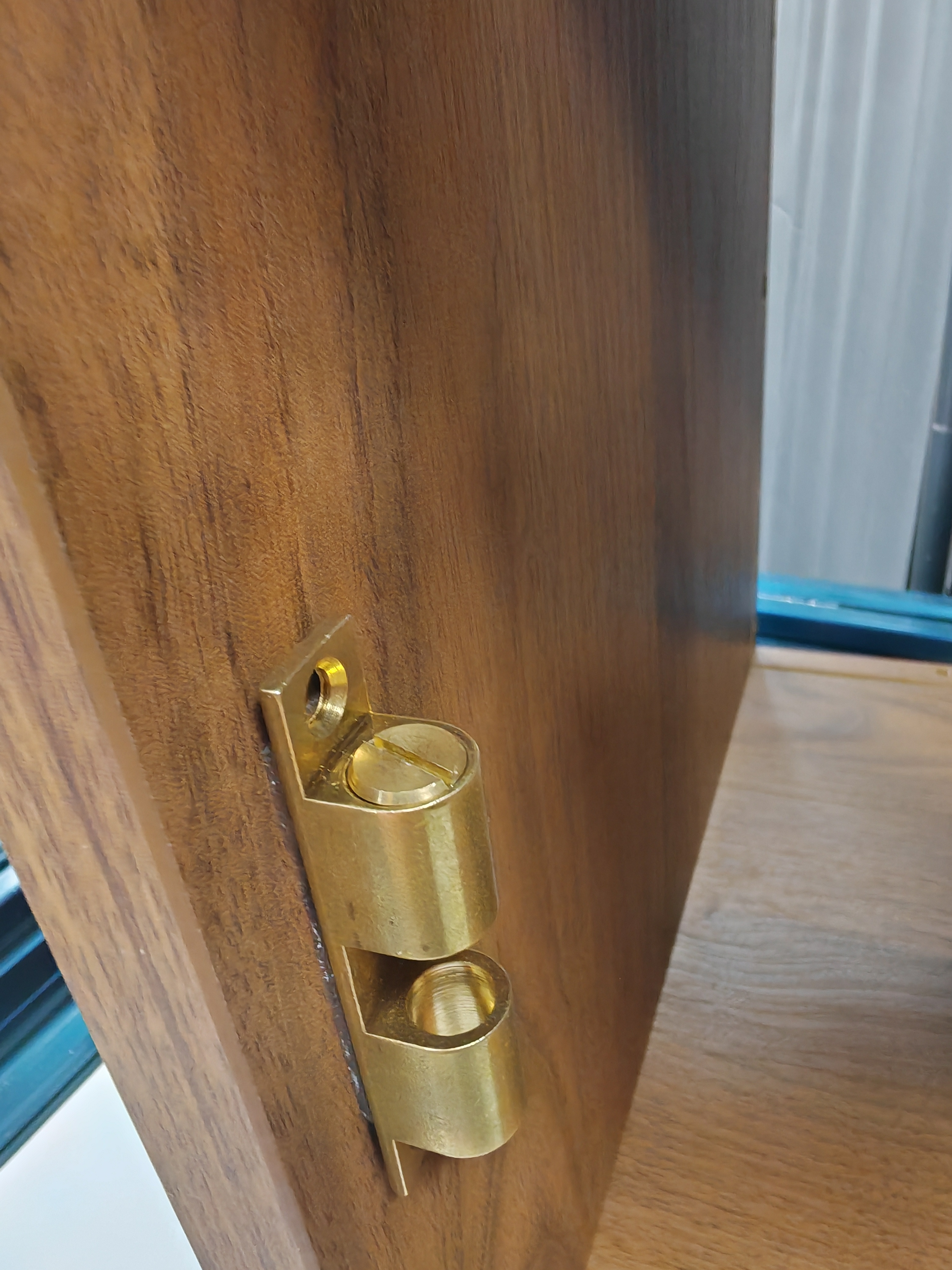
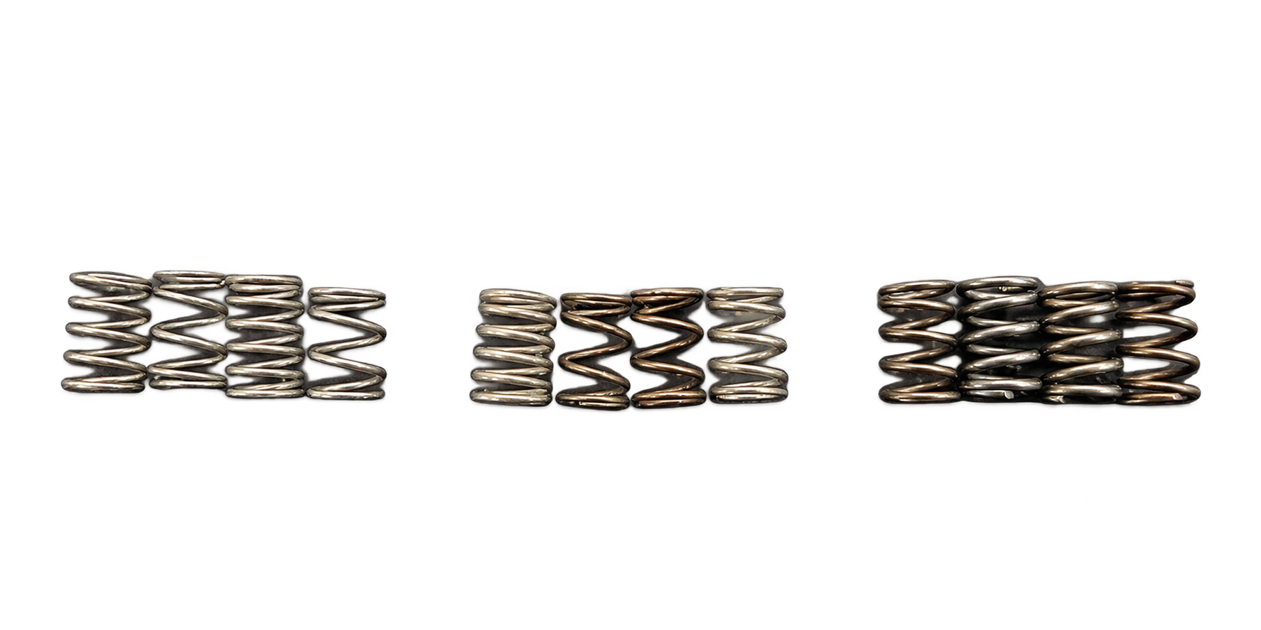
(b) Door latch and alternative springs
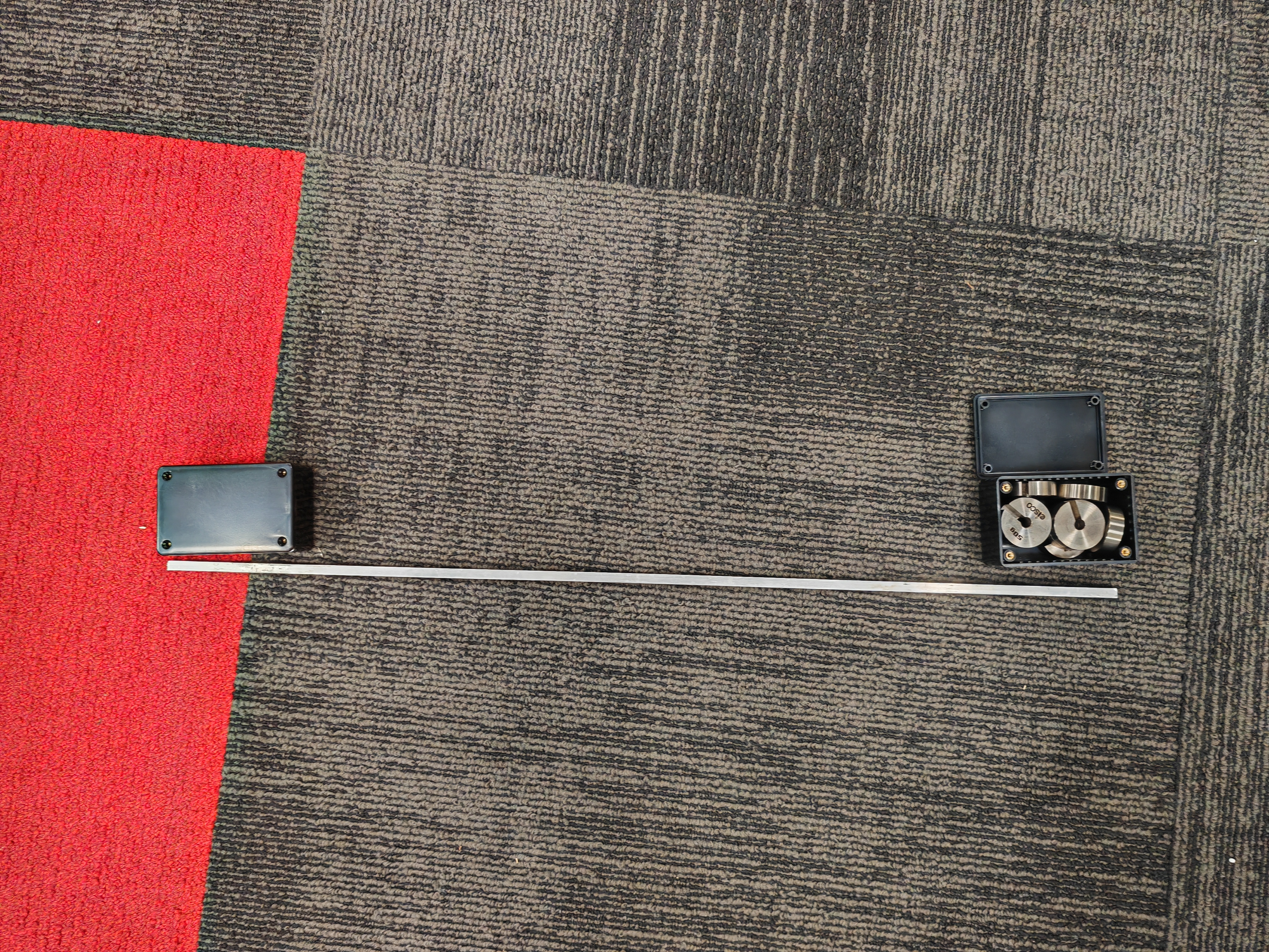
(c) Stick with adjustable end masses
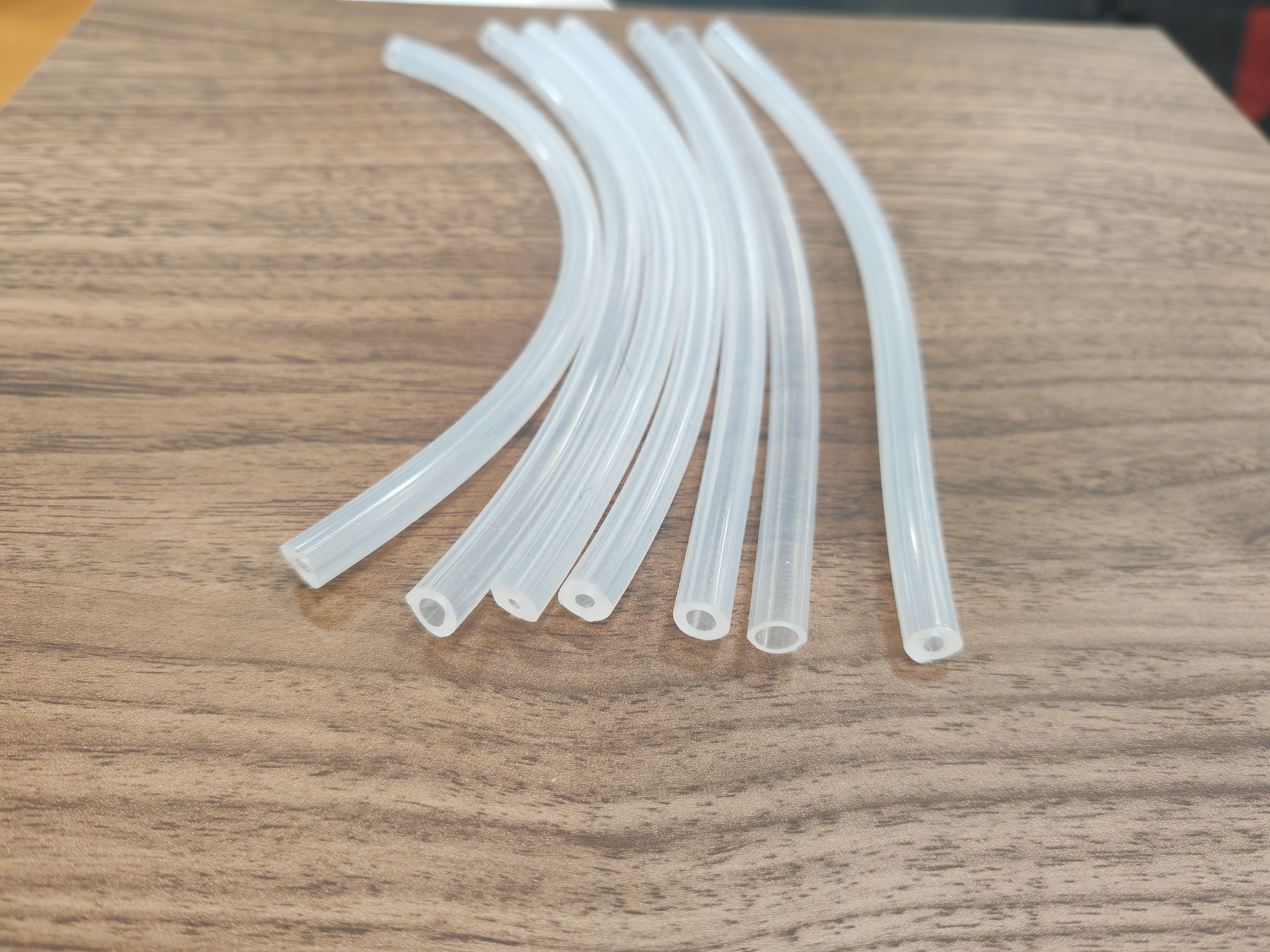
(d) Soft tubes with different stiffness and curvature
Ball Friction.
Steel beads hidden inside a ball vary its mass and resulting sliding-friction force. Track the visible center in native pixels; success means the chosen swing reaches the right-hand blue marker. The latent plot’s ball variants refer to bead loads, not directly measured friction coefficients.
Door Close.
Replace a spring-loaded latch’s spring to vary closing difficulty. Track the outer door edge, not a centroid or hinge angle. Success requires the door to close fully and latch.
Stick Balance.
Vary stick-end weights and average errors at two material markers. Choose uniformly from the candidate actions predicted to balance; if none is predicted, count failure. Execute the choice and judge actual balance. Every sampled candidate set has at least one feasible balancing action.
Soft Pull.
Tubes differ in stiffness and natural curvature and may be grasped from either side. Predict the rotation angle at which an attached object starts sliding, then perform two tests at predicted angle minus and plus 6°. Success requires no sliding in the first and sliding in the second. This threshold-bracketing test is different from choosing a single target-reaching action.
Appendix D Baseline Implementation Details
Baselines share task datasets and GPU budgets but differ in conditioning and training streams. DINOv2 conditions on a sampled trajectory subset; TTT-KQV uses ordered within-environment streams.
D.1 Standard World Model
Fine-tune the BWM transformer and action encoder on pooled trajectories without a latent or deployment updates. AdamW settings match the shared-model recipe: 10⁻⁵ learning rate, 0.01 decay, 100 warmup updates, clipping 0.5 and bfloat16.
D.2 LoRA TTA
Starting from that model, add rank-eight, alpha-eight LoRA adapters to attention query/key/value/output projections. Reset adapters for each environment, adapt on its interaction videos, then freeze them for queries. The reported Friction configuration uses 50 AdamW updates at 10⁻⁴ and clipping 1; other task settings are delegated to code.
D.3 DINOv2 Context
Frozen DINOv2 frame features and a 128-D action GRU form transition features; an MLP projects them to a 32-D context. Multiple trajectory summaries are averaged before the final projection. Training samples one or two conditioning trajectories, or one to four for Soft Pull, while all sampled trajectories act as queries. Thus this comparator already trains across varying context counts. Context heads and world-model components train jointly; test-time inference uses a forward pass without gradients.
D.4 TTT-KQV
The video test-time-training baseline inserts gated two-layer MLP fast-weight modules after eight attention blocks. Ordered chunks share a flow timestep but independent noise. Key–value binding uses learned token/head-dependent step scaling and batches of at most 64 tokens; shared slow parameters learn through the outer prediction loss. At inference, reset and replay interactions separately at every denoising timestep, then branch independently for each query’s noisy tokens. No query ground truth is used, and fast states do not carry between queries or timesteps.
Equations 15–16
| (15) | ||||
| (16) |
Appendix E Additional Experiments
Supplementary tables and plots expose interaction-count sensitivity, latent-size choice, projection methodology and compute tradeoffs.
E.1 Test-time interaction-count ablation
Going from one to two interactions raises light-switch success from 50.0% to 87.5% and door success from 22.2% to 55.6%; four gives no further success gain on these tasks. Collision improves from 61.1% through 66.7% to 72.2% for one/two/four interactions, while Soft Pull stays 81.8%. Prediction error and action success need not improve together or saturate at the same count.
| Physical error (mean) | Action success (%) | |||||
|---|---|---|---|---|---|---|
| Task | ||||||
| Mass Collision | 6.452 | 6.534 | 5.946 | 61.1 | 66.7 | 72.2 |
| Light Switch | 8.26 | 3.43 | 3.41 | 50.0 | 87.5 | 87.5 |
| Door Close | 11.337 | 7.954 | 6.889 | 22.2 | 55.6 | 55.6 |
| Soft Pull | 18.710 | 18.363 | 18.060 | 81.8 | 81.8 | 81.8 |
E.2 Latent dimensionality
On Friction with one interaction, ten held-out environments, 90 query videos and 25 reachable target decisions, 32 latent dimensions outperform 8, 16, 64 and 128 in the reported metrics. This supports the chosen size for this protocol, not a universal optimal dimension. Here video metrics explicitly use concatenated main and wrist views, whereas object errors use the main-view centroid; retain that distinction from the main-camera qualitative displays.
| Latent dim. | ADE | FDE | PSNR | SSIM | LPIPS | Success |
|---|---|---|---|---|---|---|
| 8.92 | 19.26 | 31.293 | 0.9474 | 0.0646 | 44% | |
| 7.63 | 15.90 | 29.557 | 0.9470 | 0.0614 | 64% | |
| (ours) | 3.85 | 7.59 | 31.976 | 0.9513 | 0.0495 | 72% |
| 6.86 | 13.98 | 31.692 | 0.9504 | 0.0551 | 64% | |
| 7.08 | 14.51 | 31.372 | 0.9483 | 0.0581 | 64% |
E.3 Latent-space PCA across tasks
Fit PCA separately for each task using centered training latents without feature rescaling. Project test latents with the training mean and basis; held-out latents do not influence the fit. Axes across panels are not a shared coordinate system. Colors/sizes show physical annotations only for analysis; Soft Pull’s displayed test latents use four interactions, unlike its one-interaction main evaluation.
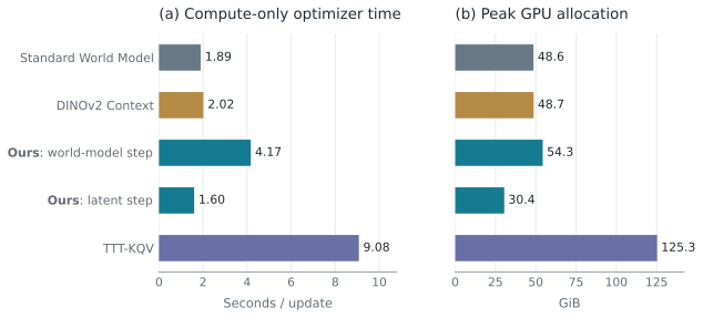
E.4 Computational efficiency
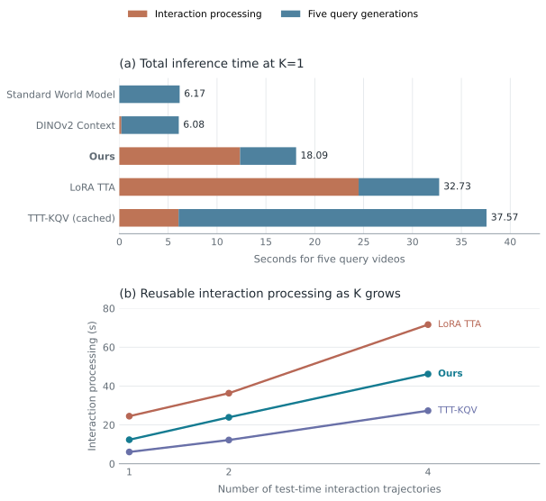
On one H200, training profiles use two warmups and ten timed updates, each with six loss-bearing chunks; they report median compute-only update time and peak allocated memory. T2-z model/latent phases cost 4.17/1.60 seconds and 54.3/30.4 GiB, respectively. With one interaction and five disjoint queries at 25 denoising steps, total compute is 18.09 seconds versus 32.73 for LoRA and 37.57 for cached TTT-KQV, but about 6.1 seconds for non-adaptive/DINOv2 methods. Loading, dataset reads and video writing are excluded; query timing includes sampling/decoding. Interaction processing is reused, and K>1 plots cover processing only, not full query generation.
Appendix F Additional Qualitative Results
Figures 12–22 preserve all selected held-out comparisons: two environments and four actions per task, except Soft Pull’s two actions per environment. Every column uses the same initial observation/action across ground truth and all five methods. The 21 original 2304×1656 comparison panels remain intact; these selected examples illustrate behavior rather than estimate failure frequency.