Overview
RePR learns image representations by fitting embedding similarities to the incremental denoising benefit provided by another image view. It uses generative prediction to reduce shortcut-driven feature suppression and tests the resulting features as conditioning for image generation.
At a glance
Relative Prediction Representations estimates a weighted pointwise-mutual-information target from a conditional generative model and trains embeddings to approximate it. Recursive feature prediction improves representations beyond pixel prediction alone. ImageNet and text-to-image experiments show useful downstream generative features, including lower generation error under selected training-compute budgets. The headline seven-to-eight-fold encoder-efficiency comparison is extrapolated from fitted scaling curves, not directly achieved by the largest trained model. Practical noise weighting, finite-model estimation, and inference architecture depart from the idealized information-theoretic objective.
1 Introduction
Discriminative self-supervision can solve its matching task using a salient shortcut while discarding other predictable features. Generative models instead need to account for detailed observations, but their internal features are not automatically convenient representations. RePR connects the two through relative prediction: how much does an additional view improve prediction of a target patch? The representation is trained to reproduce that improvement and then evaluated primarily through downstream image generation.
2 Related Work
Contrastive and noncontrastive methods learn invariances or predict features, while masked autoencoders and diffusion models predict observations. RePR follows the information-theoretic interpretation of contrastive predictive coding and implicit matrix factorization, but derives supervised embedding targets from generative prediction differences rather than a classification loss over negatives. Downstream generation uses Latent Forcing, which generates representation features before pixels.
3 Background
Pointwise mutual information measures the change in log likelihood of an observation after conditioning on another view. A contrastive optimum recovers this quantity only up to a conditioning-view-dependent offset; finite-dimensional embeddings introduce further restrictions. RePR aims to estimate useful relative prediction quantities directly. Mutual information, pointwise mutual information, and an embedding dot product are distinct objects, so the theoretical interpretation depends on the stated modeling and factorization assumptions.
Equations 1–3
| (1) |
| (2) |
| (3) |
4 Method
The method converts differences between conditional denoising errors into targets for representation similarities. It uses a practical noise-weighting schedule, predicts incremental information about one patch, and fits this target with a stop-gradient regression objective.
Equations 4–5
| (4) | ||||
| (5) |
4.1 PMI Estimation from Generative Models
The diffusion variational bound relates a log probability to integrated denoising error, following Kingma and colleagues. Subtracting conditional and unconditional errors estimates how informative a context is about a target. Equality to the true likelihood requires an optimal denoiser and appropriate endpoint/discrete-data assumptions; approximation errors need not cancel for finite trained models. The computation is therefore an estimated prediction difference, rather than an exact density-ratio oracle.
Equations 6–8
| (6) |
| (7) |
| (8) |
4.2 Timestep Weighting
The likelihood-derived weighting strongly emphasizes fine detail at small noise levels. RePR replaces it with a chosen weighting function to emphasize useful prediction scales and improve numerical behavior. This changes the target to weighted mutual-information-like prediction, not exact pointwise mutual information. The ablation using the unmodified singular weighting produces NaNs, making this practical modification central to the working method.
Equations 9–12
| (9) |
| (10) |
| (11) |
| (12) |
4.3 Bootstrapped PMI Estimation
Instead of estimating a full similarity in one expensive step, training samples a context and another patch and regresses the incremental information supplied by that patch. Exact consistent increments can telescope to a full information quantity. This motivates bootstrapping, but does not prove that finite, biased, noise-weighted estimates retain every property of exact mutual information.
Equations 13–14
| (13) |
| (14) |
4.4 Representation Objective
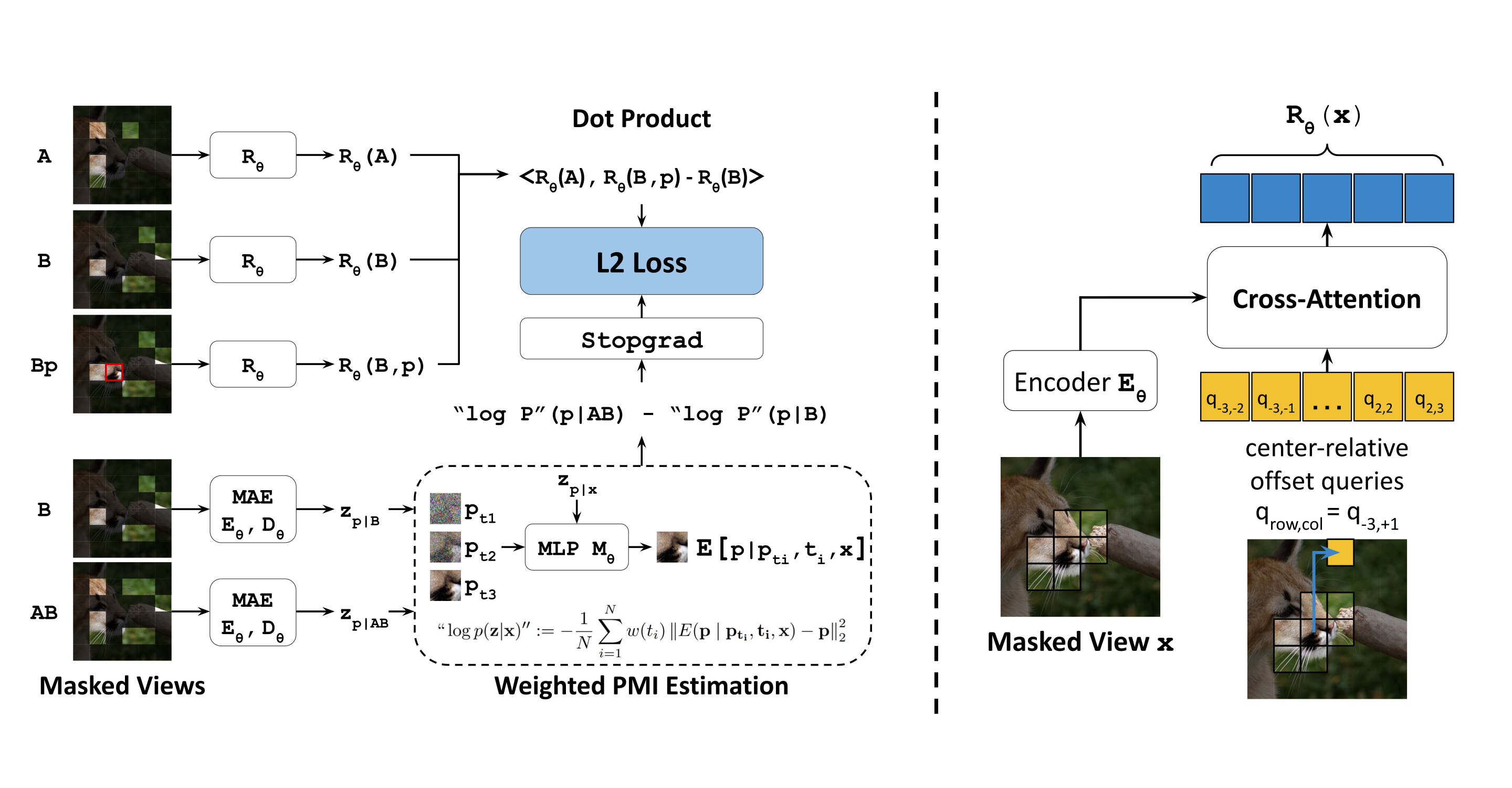
The predicted increment is a dot product between the first view’s representation and the difference between second-view representations with and without the target patch. The generative-model target is detached while the representation learns by squared error. Since mutual-information matrices need not be positive semidefinite and weighted targets may be asymmetric, separate input roles matter: the implementation marks the target patch and permits asymmetric representations. A single shared symmetric Gram matrix could not in general represent every such target.
Equation 15
| (15) | ||||
5 Architecture
A masked autoregressive prediction branch and a representation branch share an image encoder. Prediction supplies supervision during training; the final representation branch is used downstream. Its output is a spatial feature map rather than solely a global classification token.
5.1 Prediction Model
An eighteen-layer encoder feeds a six-layer prediction decoder and a small diffusion multilayer perceptron that denoises patches. This follows masked autoregressive modeling and pixel-space denoising designs, including MAR and JiT. Conditional predictions with and without a view use the same sampled noise, reducing variance in their difference.
Equation 16
| (16) |
5.2 Representing Patch Features
The representation branch adds three self-attention and three cross-attention layers to the shared eighteen-layer encoder. Relative positional structure and queries centered on patch locations produce a full patch map; an extra row and column of queries provide padding features. An additional classification-token representation objective supports linear probing. In the largest configuration, inference has twenty-four layers and width 1,024, rather than including the complete training-time prediction decoder.
5.3 Masking Strategy
Two block-masked views may overlap, while the target patch is outside both. The reported sampling masks 75–100% of view A and 93.75–100% of view B. Repeating sampled patches and views amortizes encoding. These choices control which conditional prediction problems supervise the representation; they are not a claim that all possible view/patch relationships are exhaustively observed.
5.4 Iterative Feature Prediction
After an initial pixel-prediction stage, later iterations train a new model to predict the preceding model’s features. Each stage uses the earlier representation as its target space. The reported compute includes preceding stages, so an iterative model’s final-stage epoch count alone understates its total training. Improvements are empirical and do not establish that arbitrarily many iterations monotonically improve a representation.
5.5 Joint Optimization
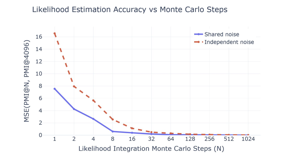
Training combines the masked generative loss with the representation regression loss, with a reported one-to-three update schedule between the joint and prediction-only components. Thirty-two Monte Carlo noise samples estimate each incremental target and add only 1.3% compute in the reported accounting. Shared noise reduces variance, while stopping gradients through the target avoids directly optimizing the predictor to make its own information estimate easier to fit.
6 Experiments
Experiments use ImageNet and GPIC, examining shortcut suppression, model/compute scaling, and image-generation quality. The primary generation comparison predicts both learned features and pixels without a separately trained perceptual/GAN image decoder. Text-to-image experiments nevertheless use an external FLAN-T5-large text encoder, and the later representation-autoencoder experiment adds separate perceptual/GAN components.
6.1 Feature Suppression
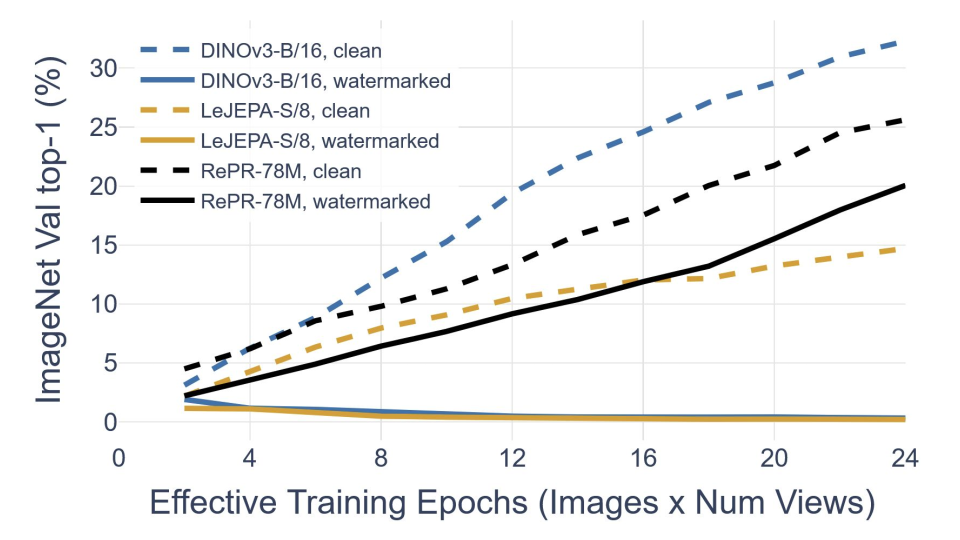
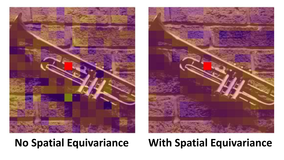
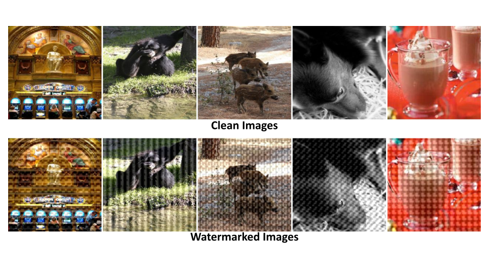
A synthetic watermark supplies each training image’s identity in every 16-by-16 patch. It makes view matching easy without understanding image content: DINOv3 and LeJEPA lose classification-probe quality under this manipulation, whereas RePR remains useful. This is evidence against one constructed feature-suppression failure mode, not a universal robustness guarantee for real-world shortcuts, distribution shifts, or all contrastive architectures.
6.2 Scaling Laws
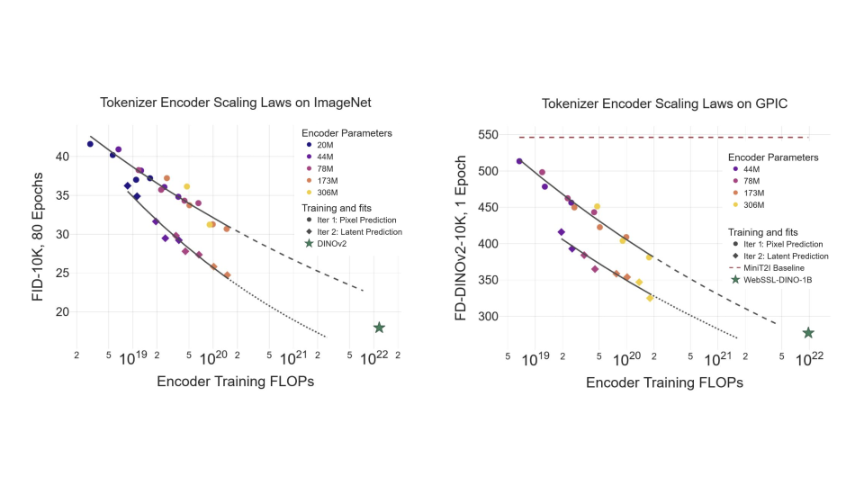
At fixed depth, encoder widths span roughly twenty to 306 million inference parameters, with training budgets varying by about two orders of magnitude. Features condition a fixed downstream generator: ImageNet evaluation uses JiT-B trained for eighty epochs and FID on ten thousand samples; GPIC uses MiniT2I and a DINOv2-feature Fréchet distance after one GPIC epoch. These metrics and datasets are not directly interchangeable.
The best measured RePR ImageNet value in the scaling table is FID 24.73, versus 17.95 for the referenced DINO feature baseline; the best listed GPIC distance is 325 versus 277.1 for the web-scale reference. The claimed seven-to-eight-fold encoder compute reduction extrapolates fitted curves to those reference scores. It is not an experimentally reached equality. The largest ImageNet models overfit after about two hundred epochs, and some individual longer runs regress slightly, so the observed scaling is not uniformly monotonic.
6.3 Compute Optimal Generation
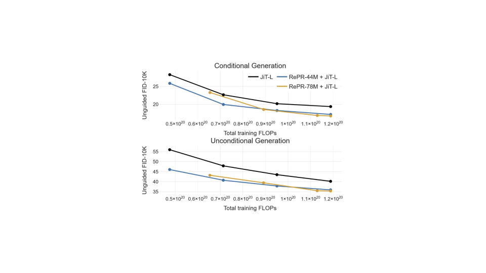
At a fixed total budget, spending some training compute on learned representation features improves a Latent Forcing generator over directly generating pixels. The medium-budget experiment allocates about twenty or thirty-five percent to two-stage forty-four- or seventy-eight-million-parameter encoders. At the larger guided setting, a seventy-eight-million-parameter, three-stage RePR encoder plus a JiT-L generator gives FID 2.18 and Inception Score 338.4 at approximately 3.49×10²⁰ training FLOPs, compared with pixel JiT-L at FID 2.36 and Inception Score 298.5 for 3.57×10²⁰.
The three encoder stages total 830 effective epochs, and guidance and the small autoguidance model are included in the reported accounting. Compute is approximated as six times parameter count times training tokens, excluding self-attention operations. It is not measured wall-clock cost or a complete inference-cost comparison, and “compute optimal” applies to the tested configurations and budget range.
6.4 Ablation Studies
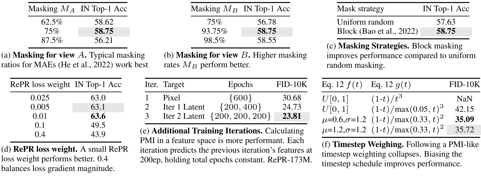
Mask rates, block masking, representation-loss weight, recursive stages, and noise weighting all affect performance. Some ablations use linear-probe accuracy as a proxy rather than downstream generation. At six hundred total epochs, one, two, and three representation stages yield generation FIDs 30.68, 24.73, and 23.81. Excessive representation-loss weights substantially reduce probe accuracy. The exact likelihood-style singular noise weighting fails numerically; clamped or smoothly reweighted alternatives train, with nontrivial sensitivity to the sampling schedule. The tables retain every setting rather than presenting a single successful recipe as inevitable.
6.5 GAN+LPIPS Decoding
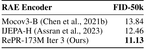
A separate experiment uses representation autoencoders with perceptual and adversarial reconstruction losses. After twenty epochs of DiT-XL generation training, the listed RePR encoder gives FID 11.13, versus 12.46 for I-JEPA-H and 13.84 for MoCo v3-B. This compares roughly matched encoder-training budgets, not a setting free of external perceptual-model costs. The cited perceptual/GAN component alone has substantial external training compute. Appendix reconstruction results also favor RePR on rFID and PSNR, while using separate decoder training and different final-stage/total-epoch conventions.

7 Conclusion
Relative generative prediction is a useful supervision signal for representations, and the experiments support recursive feature learning and allocating some generation-training compute to representations. Limits include approximate finite-model density estimates, manually chosen noise/masking schedules, idealized factorization arguments, extrapolated scaling claims, and overfitting at larger ImageNet budgets. The work chiefly tests generative utility and a synthetic shortcut stress test; it does not establish optimal features for every downstream perception or control task.
Acknowledgments
The acknowledgments identify NSF graduate fellowship support and computing support from Rhoda AI, together with feedback from colleagues.
AI use statement
The authors disclose AI assistance for coding, visualization, boilerplate, proof checking, readability, and search. They state that authors reviewed the outputs and developed the central algorithmic ideas themselves.
Appendix A Appendix
The appendix retains the exact training pseudocode, reconstruction experiments, implementation settings, theoretical qualifications, qualitative generations, watermark construction, and complete raw scaling tables.
A.1 Algorithm
The original algorithm is preserved as an indented code block. It encodes the two views and their union, predicts masked content, estimates the incremental denoising benefit under a no-gradient block with shared noise, and fits the representation increment. The final loss adds the generative term and a weighted representation-regression term. All variable names, indexing, and line breaks remain available for checking the operational meaning of the equations.
Minimal Implementation, see Sec. 5 for details. : mask for . : index of . : Number of Monte Carlo integration steps. Efficiency-only parameters and omitted for brevity. For feature prediction, the MAR target is replaced with and is replaced with
A, B, AB, p, m_AB, p_i = get_masks(X)
a, b, ab, bp = E(A), E(B), E(AB), E(B, p)
d_ab, d_b = D(ab), D(b)

x = X[m_AB]
t, eps = sample_t_eps(x)
x_t = (1 - t) * x + t * eps
x_pred = M(x_t, t, d_ab[m_AB])
mar_loss = mean(w(t) * (x_pred - x)**2)

with no_grad():
  t, eps = sample_t_eps(p, N)
  p_t = (1 - t) * repeat(p, N) + t * eps
  p_ab = M(p_t, t, d_ab[p_i])
  p_b = M(p_t, t, d_b[p_i])
  pmi = mean(g(t)*((p_b-p)**2-(p_ab-p)**2))

pred = dot(R(a), R(bp) - R(b))
repr_loss = mean((pred - pmi)**2)

loss = mar_loss + loss_weight * repr_loss
A.2 Additional Experiments
The additional reconstruction comparison reports RePR-B third-stage rFID 0.47 and PSNR 21.72, versus DINO’s 0.49 and 18.09 with the specified decoder setup. Reconstruction fidelity and downstream sample generation are different measurements. The table’s six-hundred-epoch label refers to the last encoder stage; the corresponding cumulative three-stage training can total 1,030 epochs, which matters when comparing encoder budgets.
| Model | rFID | Reconstruction PSNR |
|---|---|---|
| DINOv2-B (Oquab et al., 2024) | 0.49 | 18.09 dB |
| RePR-B Iter. 3 600ep (Ours) | 0.47 | 21.72 dB |
A.3 Implementation Details
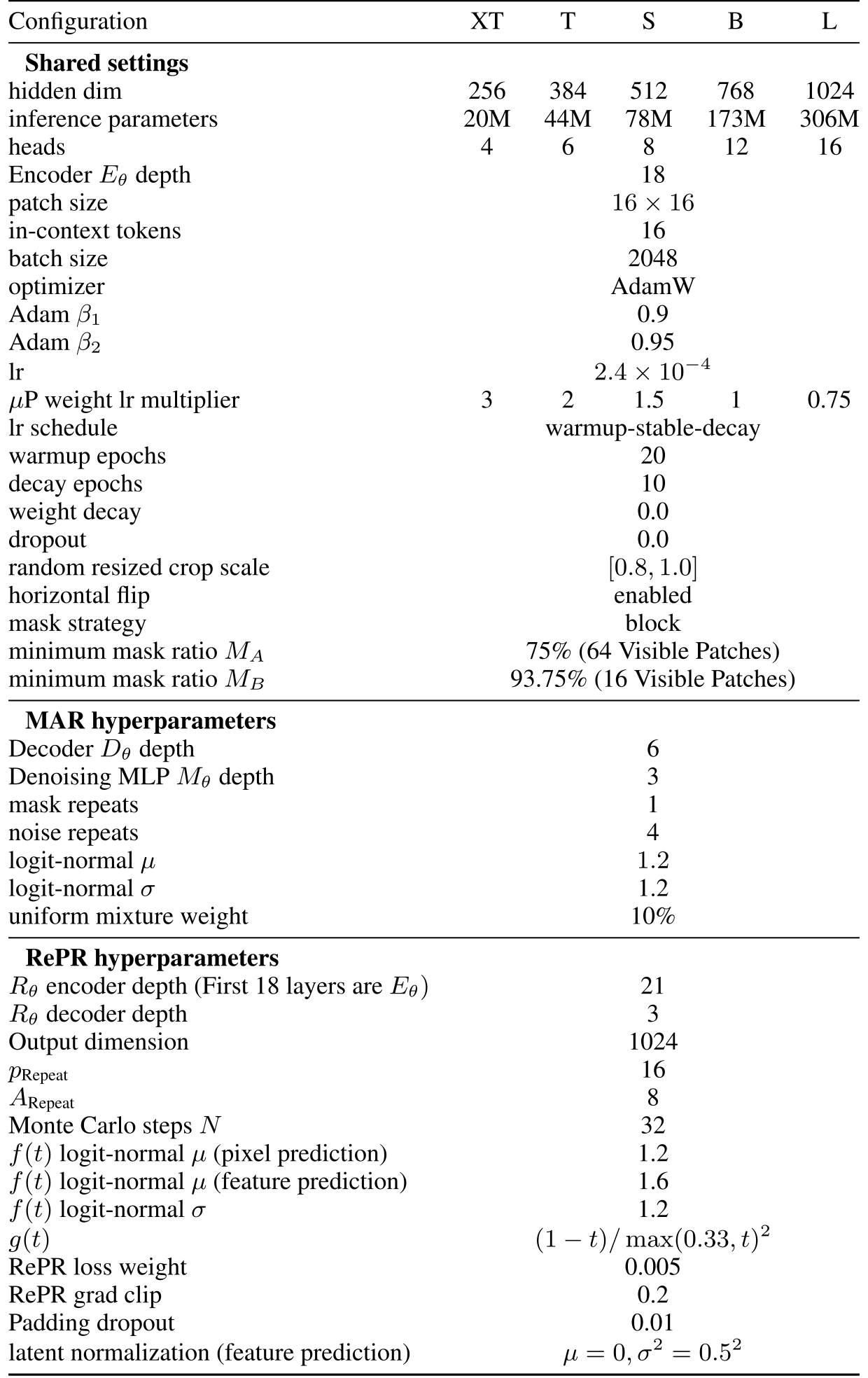
Reported training uses batch size 2,048, AdamW, base learning rate 0.00024 with width-dependent parameterization, no weight decay or dropout, and gradient clipping at 0.2. The representation-loss coefficient is 0.005. The prediction target standard deviation is scaled to 0.5 for feature prediction; pixel and feature stages use different logit-normal time means. The practical weighting is proportional to (1−t)/max(0.33,t)², with thirty-two noise samples. Effective epochs count image views relative to ImageNet size, not simply optimizer steps.
All model, masking, and generation settings are retained in the original tables. Guidance uses the specified time interval, classifier-free scale, and autoguidance settings; these are part of the reported best generation configuration. The text-to-image setup includes a pretrained FLAN-T5-large text encoder. Source HTML misrenders several configuration and numerical tables as positioned spans, so native PDF vector table bodies replace those broken conversions while retaining captions and anchors.
A.4 Properties of PMI
The appendix discusses idealized reconstruction from prediction-based information. Its argument assumes uncorrupted conditioning observations, support for the relevant pixel values, arbitrarily small noise, and access to an idealized search over possible target values. It motivates preserving predictable information but does not prove lossless finite-dimensional practical encodings under masking and imperfect optimization. Pointwise-information matrices can be indefinite, and weighted prediction information can be asymmetric; role-dependent factors address this expressivity issue rather than making a shared symmetric dot-product matrix universally sufficient.
| config | ImageNet | ImageNet | GPIC |
|---|---|---|---|
| decoder | JiT-B (Li and He, 2026) | JiT-L (Li and He, 2026) | MiniT2I (Wang et al., 2026) |
| hidden dim | 768 | 1024 | 768 |
| backbone depth | 12 | 20 | 17 |
| output experts Baade et al. (2026) | 2 1024 dim | 2 1024 dim | - |
| text encoder | - | - | FLAN-T5-large |
| max text tokens | - | - | 128 |
| epochs | 80 | ||
| global batch size | 1024 | ||
| optimizer | AdamW | ||
| peak lr | |||
| lr schedule | constant after warmup | ||
| warmup epochs | 5 | ||
| weight decay | 0.0 | ||
| pixel time | |||
| pixel time | 0.8 | ||
| latent time | |||
| latent time | 1.0 | ||
| latent selection probability | 0.5 | ||
| latent loss weight | 1.0 | ||
| (Li and He, 2026) | 0.05 | ||
| latent normalization | |||
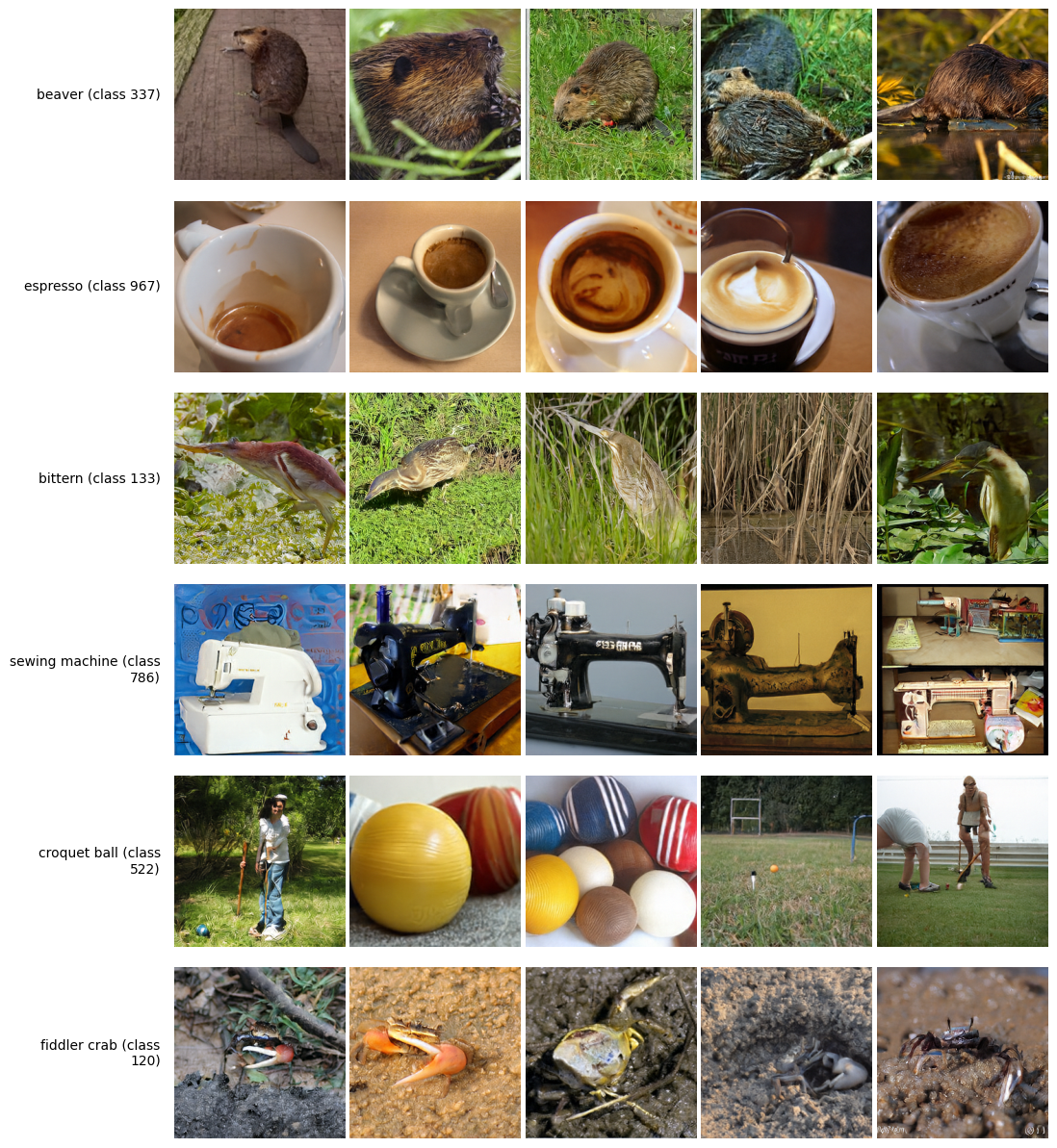
A.5 Qualitative Results
The retained image grids show generated samples from the reported representation-conditioned models. Latent Forcing jointly models feature and pixel trajectories, avoiding a fixed lossy image decoder in this evaluation. Its pixel-space generation path does not imply that the representation alone exactly reconstructs every input image.
A.6 Watermarking
Each image receives a unique synthetic watermark repeated within every image patch, creating an easy identity signal across masked views. The figure preserves the construction and examples. This deliberately strong shortcut makes the suppression experiment interpretable but differs from uncontrolled naturally occurring correlations.
A.7 Raw Numbers for Scaling Plots
The complete raw ImageNet and GPIC tables retain every listed width, parameter count, stage length, compute value, and quality score. They expose saturation, overfitting, and small nonmonotonic changes that fitted scaling curves can hide. The comparison to larger pretrained encoders uses extrapolation to their scores; it should be read alongside the measured points and the approximate FLOP accounting.
| Iteration 1: Pixel | Iteration 2: Latent | |||
| Encoder (width) | Epochs | FID | Epochs | FID |
| 20M (256) | 110 | 41.61 | 36.24 | |
| 210 | 40.19 | 34.89 | ||
| 410 | 37.01 | – | – | |
| 610 | 37.21 | – | – | |
| 44M (384) | 110 | 40.93 | 31.64 | |
| 210 | 38.20 | 29.48 | ||
| 410 | 36.07 | 29.22 | ||
| 610 | 34.82 | – | – | |
| 78M (512) | 110 | 38.26 | 29.81 | |
| 210 | 35.72 | 27.80 | ||
| 410 | 34.31 | 27.36 | ||
| 610 | 34.00 | – | – | |
| 173M (768) | 110 | 37.22 | 25.82 | |
| 210 | 33.73 | 24.73 | ||
| 410 | 31.27 | – | – | |
| 610 | 30.68 | – | – | |
| 306M (1024) | 110 | 36.14 | – | – |
| 211 | 31.23 | – | – | |
| Iteration 1: Pixel | Iteration 2: Latent | |||
|---|---|---|---|---|
| Encoder (width) | ImageNet Epochs-Worth | FD | ImageNet Epochs-Worth | FD |
| 44M (384) | 110 | 514 | 416 | |
| 210 | 479 | 393 | ||
| 410 | 456 | – | – | |
| 78M (512) | 110 | 498 | 384 | |
| 210 | 463 | 365 | ||
| 410 | 443 | – | – | |
| 173M (768) | 110 | 450 | 359 | |
| 210 | 423 | 354 | ||
| 410 | 409 | – | – | |
| 306M (1024) | 110 | 451 | 347 | |
| 210 | 404 | 325 | ||
| 410 | 381 | – | – | |