Overview
This edition includes the 14-page arXiv v1 and the separate 18-page appendix supplied by the authors’ project. All figure panels, tables, formal statements, proof steps, algorithms and the original video remain. The project’s main PDF has the same technical text as arXiv v1, but changes bibliography entries 7 and 53; this edition retains the arXiv bibliography and labels the supplement separately. The standalone supplement cites additional numbers without supplying their bibliography, so missing entries are not invented.
At a glance
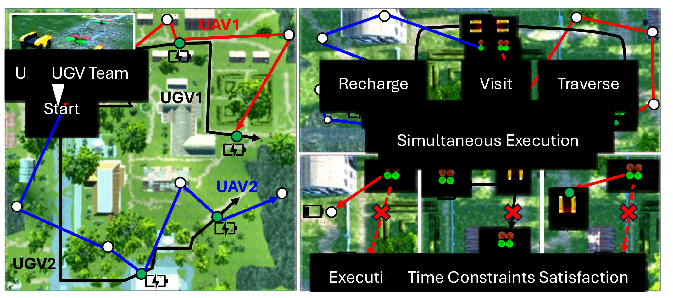
MEND plans for aerial robots that visit tasks and ground robots that support recharging along traversable routes. It learns masked action sequences from mixed-integer expert plans, removes actions rejected by symbolic energy/coordination checks, and reveals a low-entropy admissible position at each decoding step. Reported simulations achieve 100% task completion across eight mission/team settings, with lower makespan and energy than the selected baselines. A mixed-reality demonstration adds physical robot execution. The theory has narrower assumptions than an unconditional guarantee for the learned adaptive sampler.
1 Introduction
Energy-limited UAVs can cover tasks that road-constrained UGVs cannot directly reach, while the UGVs provide mobile recharge support. Coordinating task visits, ground travel and rendezvous makes their plans interdependent. MEND addresses this through a joint conditional generator with explicit execution-time admissibility checks. It generates a complete plan centrally; it does not implement decentralized online replanning for new tasks during a mission.
2 Related Work
The related work connects optimization, symbolic planning, reinforcement learning and masked generative policies. MEND’s main distinction is hard reweighting of the learned action distribution with domain-specific logical checks, followed by entropy-guided decoding under that constrained distribution.
Collaborative Planning for Multi-Robot Systems
MIP, dynamic programming and heuristic route search can coordinate tasks and recharge events, but large exact problems can be expensive. Symbolic languages express operational rules; reinforcement learning learns routing or coordination policies. The comparison does not imply that all optimization planners are inherently too slow at every problem size or that learned inference eliminates the offline expert-generation cost.
Masked Diffusion Models.
Masked diffusion progressively fills discrete action positions. Random or entropy-based reveal orders can alter sample quality. The cited information-curve analysis concerns dependence between tokens; MEND adds feasibility-aware probabilities before computing entropy. Learned probability concentration is a decoding heuristic, rather than a direct estimate of task makespan or a calibrated certificate of correctness.
3 Preliminaries
The preliminaries define absorbing-mask corruption, learned conditional denoising and symbolic predicates/actions. The original transition and posterior formulas remain. A symbolic rule evaluates current modeled context; physical validity still depends on the predicates, state estimates and simulator matching the actual environment.
MDM Inference Scheduling
An inference schedule records which positions have been revealed. Entropy-guided decoding chooses among still-masked positions using the model’s conditional distribution. MEND later computes this entropy after inadmissible actions are removed. Low entropy means a concentrated predicted action distribution; it does not by itself mean a globally optimal route.
4 Approach
The approach represents tasks, robots and rendezvous paths as a heterogeneous graph, predicts a joint action sequence and applies symbolic checks during generation. It combines parallel robot execution with centralized joint-plan inference. The logical checks target task affordability, support movement and recharge coordination.
Problem Definition
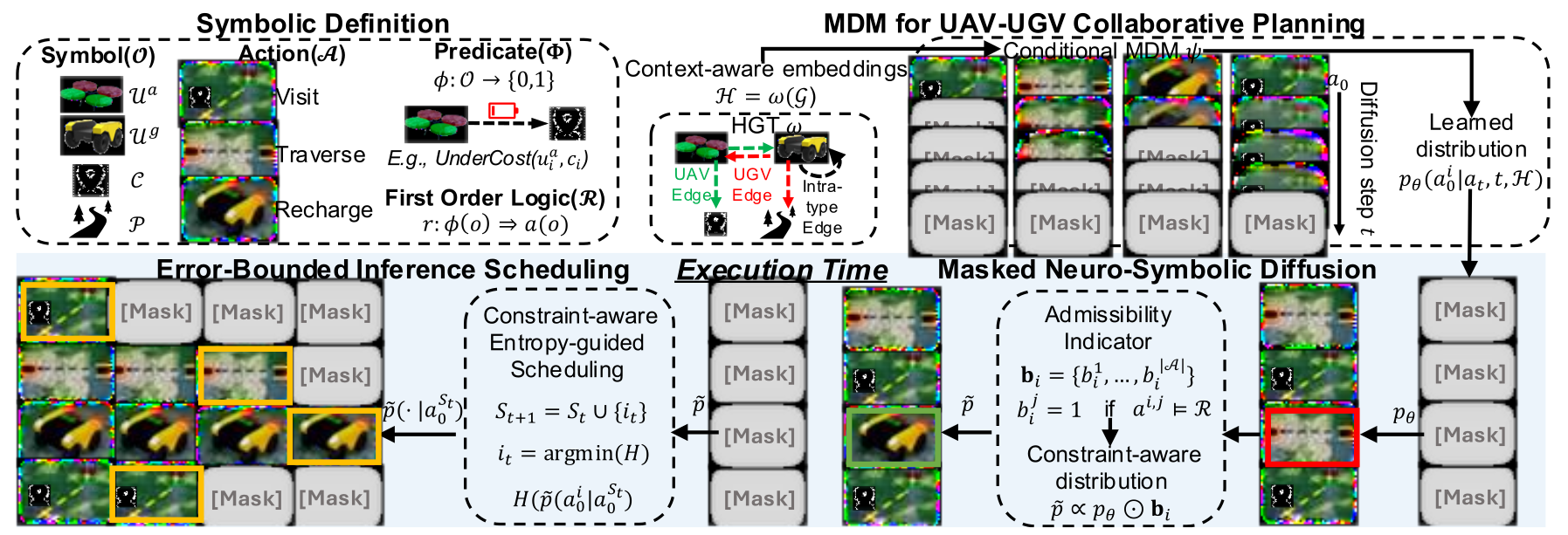
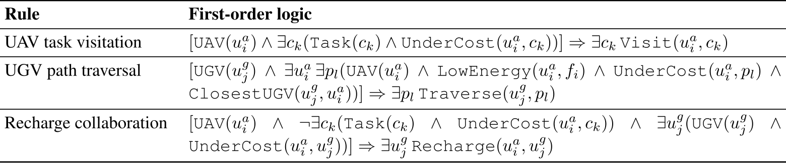
UAV task nodes store location/visit status; rendezvous nodes encode traversable ground paths; UAV nodes include location and energy; UGV context includes its own state and UAV locations. Typed and proximity relations connect the entities. Grounded Visit, Traverse and Recharge actions form the discrete vocabulary. The printed FOL examples are existential implications, while the implementation additionally uses explicit admissibility masks; the table alone is not a complete executable specification of every allowed action.
MDM for Collaborative Planning of Heterogeneous Robots
A heterogeneous graph Transformer produces context embeddings through same-type and cross-type attention. A conditional masked model then predicts action tokens from the partially masked sequence, timestep and graph context. Training minimizes the clean-token negative log likelihood at masked positions using MIP-generated demonstrations. The learned distribution is an approximation to those experts, rather than an exact solver of the original combinatorial problem.
Execution-Time Masked Neuro-Symbolic Diffusion
At each masked position, MEND multiplies predicted action probabilities by a Boolean admissibility vector and renormalizes. Rejected actions receive zero probability and surviving actions retain their relative probabilities. This requires nonzero predicted mass on at least one admissible action; a zero-support fallback is not specified. Appendix D describes full-sequence state simulation and tensorized fuel/visit checks. Constraint satisfaction is conditional on those masks being sound for the final joint execution; binary masking alone does not certify unmodeled dynamics or estimation error.
Execution-Time Error-Bounded Inference Scheduling
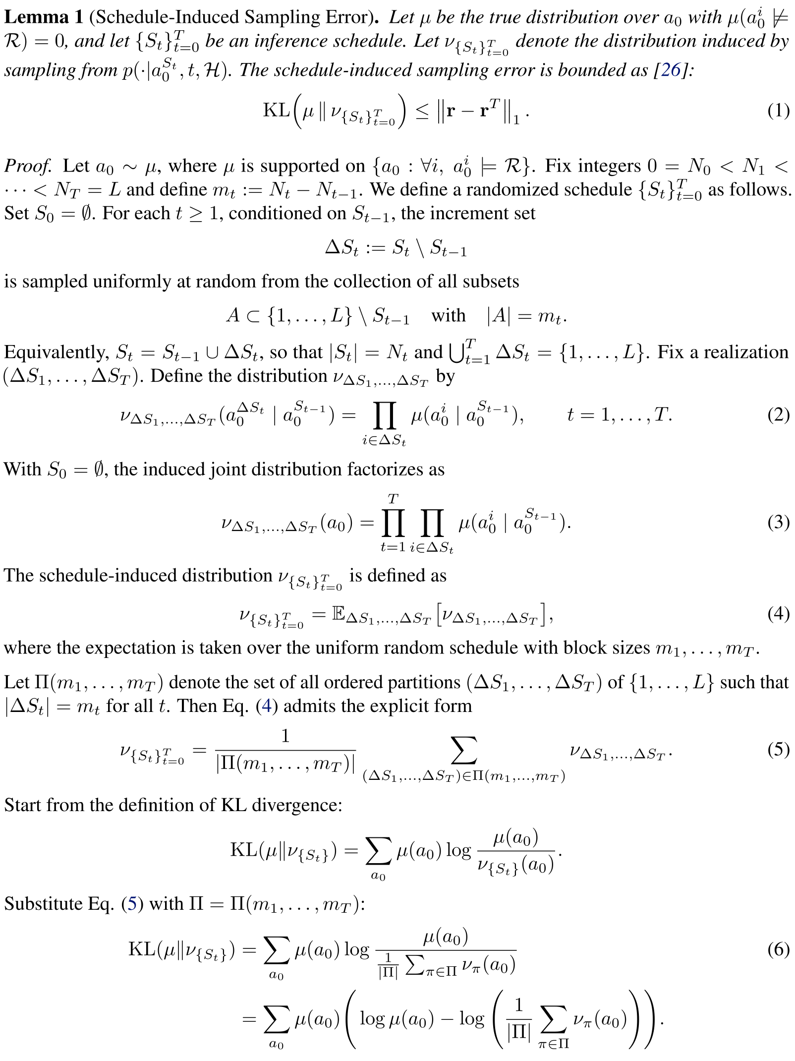
MEND reveals a position with minimum entropy under its constrained distribution. The retained Lemma 1 bounds schedule error by information-curve mismatch; Appendix B proves it for exact data conditionals and a uniformly randomized block schedule. The proof does not include learned-denoiser error or establish the same bound for the adaptive minimum-entropy schedule. Theorem 1’s KL identity is valid for global conditioning on a feasible set, as explicitly defined in supplementary Eq. 32. History-dependent token masks generally use different normalizers, so equivalence to that globally conditioned joint law requires an additional argument. These results do not certify globally optimal makespan.
Lemma 1 (Schedule-Induced Sampling Error).
Let be the true distribution over with , and let be an inference schedule. Let denote the distribution induced by sampling from . The schedule-induced sampling error is bounded as [26]:
Equation 1
| (1) |
Theorem 1 (Error Reduction via Constraint-Aware Scheduling).
5 Experiments
Experiments compare three heuristic planners and two masked-diffusion baselines across two task/path workloads and four team configurations. They also inspect new road/depot layouts, a scanned campus map, physical robots, inference speed and selected ablations. The appendix supplies training details and additional variability tables.
Experimental Setups
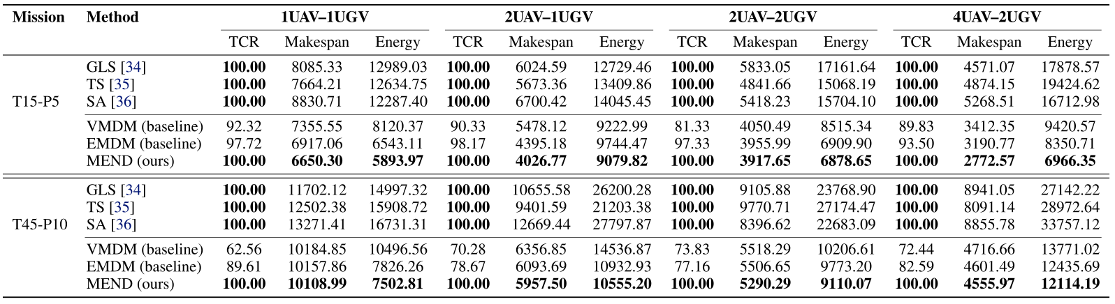
Unity/ROS simulations use Starling 2 UAV and Warthog UGV models on a 10 km square region. Missions contain 15 tasks/5 paths or 45 tasks/10 paths, with 1–4 UAVs and 1–2 UGVs. Main speeds are 10 and 4.5 m/s; capacities are 287.7 and 36,810 kJ. Task Completion Rate is the fraction of required tasks completed, not automatically a mission success probability. Makespan is evaluated only on the intersection of cases all compared methods finish; the supplement applies this restriction to energy comparisons as well. Energy sums the entire team’s mission consumption. The exact retained successful-subset sizes are not reported.

Accessible table and original mathematical notation
Mission
Method
1UAV–1UGV
2UAV–1UGV
2UAV–2UGV
4UAV–2UGV
TCR
Makespan
Energy
TCR
Makespan
Energy
TCR
Makespan
Energy
TCR
Makespan
Energy
T15-P5
GLS [34]
100.00
8085.33
12989.03
100.00
6024.59
12729.46
100.00
5833.05
17161.64
100.00
4571.07
17878.57
TS [35]
100.00
7664.21
12634.75
100.00
5673.36
13409.86
100.00
4841.66
15068.19
100.00
4874.15
19424.62
SA [36]
100.00
8830.71
12287.40
100.00
6700.42
14045.45
100.00
5418.23
15704.10
100.00
5268.51
16712.98
VMDM (baseline)
92.32
7355.55
8120.37
90.33
5478.12
9222.99
81.33
4050.49
8515.34
89.83
3412.35
9420.57
EMDM (baseline)
97.72
6917.06
6543.11
98.17
4395.18
9744.47
97.33
3955.99
6909.90
93.50
3190.77
8350.71
MEND (ours)
100.00
6650.30
5893.97
100.00
4026.77
9079.82
100.00
3917.65
6878.65
100.00
2772.57
6966.35
T45-P10
GLS [34]
100.00
11702.12
14997.32
100.00
10655.58
26200.28
100.00
9105.88
23768.90
100.00
8941.05
27142.22
TS [35]
100.00
12502.38
15908.72
100.00
9401.59
21203.38
100.00
9770.71
27174.47
100.00
8091.14
28972.64
SA [36]
100.00
13271.41
16731.31
100.00
12669.44
27797.87
100.00
8396.62
22683.09
100.00
8855.78
33757.12
VMDM (baseline)
62.56
10184.85
10496.56
70.28
6356.85
14536.87
73.83
5518.29
10206.61
72.44
4716.66
13771.02
EMDM (baseline)
89.61
10157.86
7826.26
78.67
6093.69
10932.93
77.16
5506.65
9773.20
82.59
4601.49
12435.69
MEND (ours)
100.00
10108.99
7502.81
100.00
5957.50
10555.20
100.00
5290.29
9110.07
100.00
4555.97
12114.19


Results under Various Task and Team Configurations
MEND reports 100% task completion in all eight settings. Its makespans for 15-task teams are 6650.30, 4026.77, 3917.65 and 2772.57 seconds, and for 45-task teams 10108.99, 5957.50, 5290.29 and 4555.97 seconds. The full table retains all baseline task fractions, makespans and energy values. Lower conditional makespan should be read alongside completion rate, since incomplete cases are excluded from that comparison. Selected trajectories illustrate parallel aerial work and supporting ground recharge routes.
Results on Unseen Simulation and Real-World Environments
New city/suburban layouts change road networks and the depot. The campus experiment uses an unseen 3D LiDAR map with robot models in simulation; it is not an outdoor hardware trial. The campus description changes the UAV battery to 106.6 kJ and prints consumption as 198.6 kJ/h at 10 m/s, with the UGV at 2680.3 kJ/h at 5 m/s. Those stated units/configurations are retained rather than silently reconciled with the earlier speed-dependent model. New-map evidence is largely qualitative rather than a complete held-out-map success table.


Case Studies on Physical UAV-UGV Teams
The physical case uses two Crazyflie UAVs and two Limo UGVs controlled through ROS2, a projected mixed-reality environment and motion capture. It shows a 15-task mission with coordinated visit/travel/recharge events. The manuscript does not provide a repeated physical-trial success count or enough charging-hardware detail to infer that each depicted recharge is a measured electrical battery transfer. This validates selected robot coordination behavior under the experiment’s localization/environment setup.
Scalability
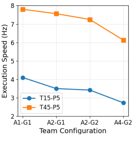
The prose reports inference decreasing from 7.8 Hz for the smallest mission to 2.8 Hz for the largest. Figure 8 instead labels the lower roughly 4.1→2.8-Hz curve T15-P5 and the upper 7.8→6.1-Hz curve T45-P5, differing from both that prose and the T45-P10 mission designation. The original plot is preserved without swapping its labels. The 45-task/four-UAV/two-UGV comparison gives MEND 4555.97-second makespan, 12114.19-kJ energy and 2.830-Hz inference, versus MIP 4369.18, 11433.37 and 0.006 Hz. These are about 4.28%/5.95% higher objectives at 472× inference speed. The expert MIP’s printed objective is total travel distance, so ‘near optimal’ does not certify optimality separately for makespan and energy. Offline data generation and model training are outside the inference timing.
Ablation Study
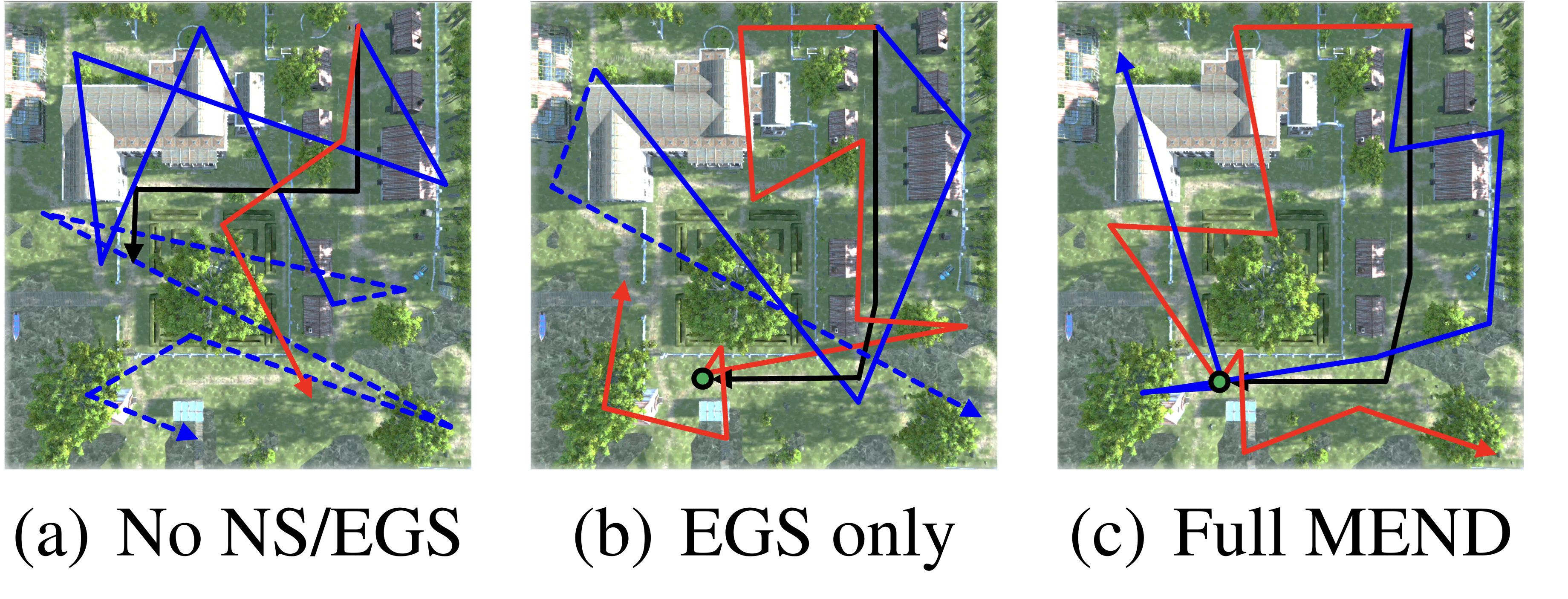
Figure 9 contrasts no symbolic masking/no entropy guidance, entropy guidance alone and full MEND. Dashed paths mark constraint violations in the first two examples. These selected plans support the role of symbolic masking but do not give a repeated quantitative factorial ablation or isolate every interaction between the two components.
6 Limitation
Fixed-length plans and static task sets limit insertion of new tasks during execution. Although robots execute in parallel, plan inference is centralized and assumes reliable communication/context. Decentralized graph-factorized inference and variable-length generation are future work.
7 Conclusion
The empirical contribution is a learned joint planner with explicit domain masks and constraint-aware reveal ordering. It improves the reported conditional metrics and completion fractions in the tested simulation settings, with selected physical coordination examples. Its theoretical conditioning identity should remain distinct from a guarantee for all learned adaptive masked generation or physical execution.
Acknowledgments
The acknowledgment lists NSF, U.S. Army Research Laboratory and DARPA support. The complete 75-entry arXiv v1 bibliography is retained.
Appendix A · Mathematical notation
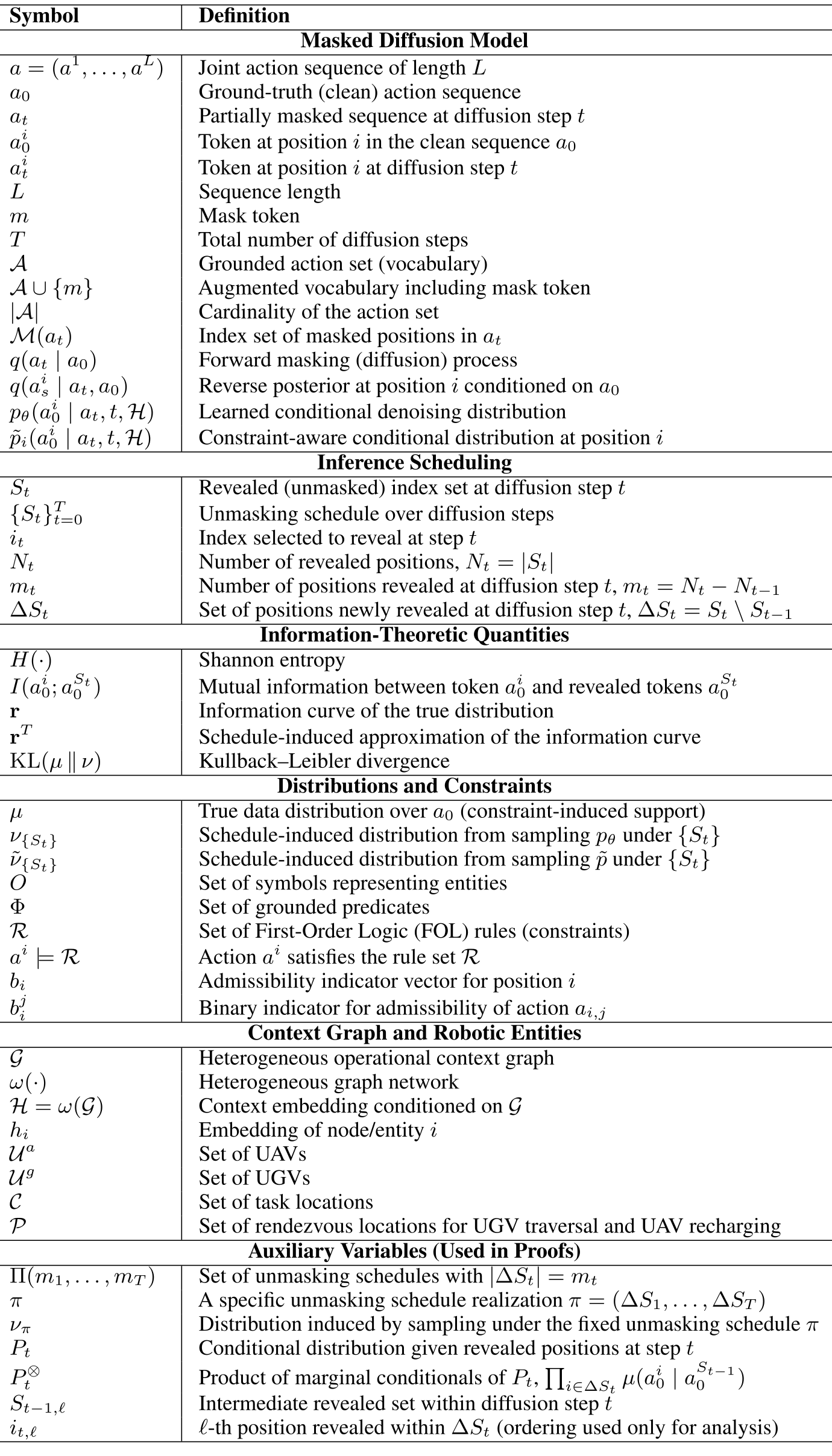
Supplementary Table 1 retains all mathematical symbols and their roles, including schedule block sizes, distributions, admissibility vectors, graph entities and intermediate revealed sets. Main and supplementary numbering remain separate.
Selectable PDF text; mathematical layout is preserved above
Symbol
Definition
Masked Diffusion Model
a = (a1, . . . , aL)
Joint action sequence of length L
a0
Ground-truth (clean) action sequence
at
Partially masked sequence at diffusion step t
ai
0
Token at position i in the clean sequence a0
ai
t
Token at position i at diffusion step t
L
Sequence length
m
Mask token
T
Total number of diffusion steps
A
Grounded action set (vocabulary)
A →{m}
Augmented vocabulary including mask token
|A|
Cardinality of the action set
M(at)
Index set of masked positions in at
q(at | a0)
Forward masking (diffusion) process
q(ai
s | at, a0)
Reverse posterior at position i conditioned on a0
pω(ai
0 | at, t, H)
Learned conditional denoising distribution
˜pi(ai
0 | at, t, H)
Constraint-aware conditional distribution at position i
Inference Scheduling
St
Revealed (unmasked) index set at diffusion step t
{St}T
t=0
Unmasking schedule over diffusion steps
it
Index selected to reveal at step t
Nt
Number of revealed positions, Nt = |St|
mt
Number of positions revealed at diffusion step t, mt = Nt ↑Nt→1
!St
Set of positions newly revealed at diffusion step t, !St = St \ St→1
Information-Theoretic Quantities
H(·)
Shannon entropy
I(ai
0; aSt
0 )
Mutual information between token ai
0 and revealed tokens aSt
0
r
Information curve of the true distribution
rT
Schedule-induced approximation of the information curve
KL(µ ↓ω)
Kullback–Leibler divergence
Distributions and Constraints
µ
True data distribution over a0 (constraint-induced support)
ω{St}
Schedule-induced distribution from sampling pω under {St}
˜ω{St}
Schedule-induced distribution from sampling ˜p under {St}
O
Set of symbols representing entities
”
Set of grounded predicates
R
Set of First-Order Logic (FOL) rules (constraints)
ai |= R
Action ai satisfies the rule set R
bi
Admissibility indicator vector for position i
bj
i
Binary indicator for admissibility of action ai,j
Context Graph and Robotic Entities
G
Heterogeneous operational context graph
ε(·)
Heterogeneous graph network
H = ε(G)
Context embedding conditioned on G
hi
Embedding of node/entity i
Ua
Set of UAVs
Ug
Set of UGVs
C
Set of task locations
P
Set of rendezvous locations for UGV traversal and UAV recharging
Auxiliary Variables (Used in Proofs)
#(m1, . . . , mT )
Set of unmasking schedules with |!St| = mt
ϑ
A specific unmasking schedule realization ϑ = (!S1, . . . , !ST )
ωε
Distribution induced by sampling under the fixed unmasking schedule ϑ
Pt
Conditional distribution given revealed positions at step t
P ↑
t
Product of marginal conditionals of Pt, !
i↓!St µ(ai
0 | a
St→1
0
)
St→1,ϑ
Intermediate revealed set within diffusion step t
it,ϑ
ϖ-th position revealed within !St (ordering used only for analysis)
Appendix B.1 · Schedule-induced sampling error
The proof first averages over uniform ordered partitions, uses Jensen’s inequality, and decomposes KL error into within-block conditional total correlation. Exact data conditionals are then related to the information curve, giving the L1 mismatch bound. This analysis assumes the oracle conditionals and specified random schedule; there is no extra term controlling the trained network’s approximation error or proof for adaptively choosing the next position from its predicted entropy. The complete proof, including Eqs. 1–26 and all unnumbered steps, is preserved in original vector layout.
Selectable PDF text; mathematical layout is preserved above
Lemma 1 (Schedule-Induced Sampling Error). Let µ be the true distribution over a0 with µ(ai
0 →|=
R) = 0, and let {St}T
t=0 be an inference schedule. Let ω{St}T
t=0 denote the distribution induced by
sampling from p(·|aSt
0 , t, H). The schedule-induced sampling error is bounded as [26]:
KL
!
µ ↑ω{St}T
t=0
"
↓
##r ↔rT ##
1 .
(1)
Proof. Let a0 ↗µ, where µ is supported on {a0 : ↘i, ai
0 |= R}. Fix integers 0 = N0 < N1 <
· · · < NT = L and define mt := Nt ↔Nt→1. We define a randomized schedule {St}T
t=0 as follows.
Set S0 = ≃. For each t ⇐1, conditioned on St→1, the increment set
!St := St \ St→1
is sampled uniformly at random from the collection of all subsets
A ⇒{1, . . . , L} \ St→1
with
|A| = mt.
Equivalently, St = St→1 ⇑!St, so that |St| = Nt and $T
t=1 !St = {1, . . . , L}. Fix a realization
(!S1, . . . , !ST ). Define the distribution ω!S1,...,!ST by
ω!S1,...,!ST (a!St
0
| aSt→1
0
) =
%
i↑!St
µ(ai
0 | aSt→1
0
),
t = 1, . . . , T.
(2)
With S0 = ≃, the induced joint distribution factorizes as
ω!S1,...,!ST (a0) =
T
%
t=1
%
i↑!St
µ(ai
0 | aSt→1
0
).
(3)
The schedule-induced distribution ω{St}T
t=0 is defined as
ω{St}T
t=0 = E!S1,...,!ST
&
ω!S1,...,!ST
'
,
(4)
where the expectation is taken over the uniform random schedule with block sizes m1, . . . , mT .
Let ”(m1, . . . , mT ) denote the set of all ordered partitions (!S1, . . . , !ST ) of {1, . . . , L} such that
|!St| = mt for all t. Then Eq. (4) admits the explicit form
ω{St}T
t=0 =
1
|”(m1, . . . , mT )|
(
(!S1,...,!ST )↑”(m1,...,mT )
ω!S1,...,!ST .
(5)
Start from the definition of KL divergence:
KL(µ↑ω{St}) =
(
a0
µ(a0) log
µ(a0)
ω{St}(a0).
Substitute Eq. (5) with ” = ”(m1, . . . , mT ):
KL(µ↑ω{St}) =
(
a0
µ(a0) log
µ(a0)
1
|”|
)
ω↑” ωω(a0)
(6)
=
(
a0
µ(a0)
*
log µ(a0) ↔log
*
1
|”|
(
ω↑”
ωω(a0)
++
.
Selectable PDF text; mathematical layout is preserved above
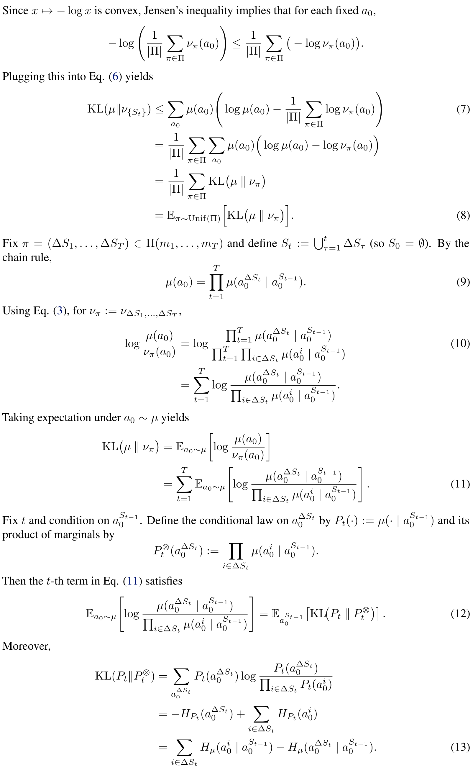
Since x ⇓⇔↔log x is convex, Jensen’s inequality implies that for each fixed a0,
↔log
*
1
|”|
(
ω↑”
ωω(a0)
+
↓
1
|”|
(
ω↑”
,
↔log ωω(a0)
-
.
Plugging this into Eq. (6) yields
KL(µ↑ω{St}) ↓
(
a0
µ(a0)
*
log µ(a0) ↔1
|”|
(
ω↑”
log ωω(a0)
+
(7)
=
1
|”|
(
ω↑”
(
a0
µ(a0)
!
log µ(a0) ↔log ωω(a0)
"
=
1
|”|
(
ω↑”
KL
,
µ ↑ωω
-
= Eω↓Unif(”)
.
KL
,
µ ↑ωω
-/
.
(8)
Fix ε = (!S1, . . . , !ST ) ↖”(m1, . . . , mT ) and define St := $t
ε=1 !Sε (so S0 = ≃). By the
chain rule,
µ(a0) =
T
%
t=1
µ(a!St
0
| aSt→1
0
).
(9)
Using Eq. (3), for ωω := ω!S1,...,!ST ,
log µ(a0)
ωω(a0) = log
T
t=1 µ(a!St
0
| aSt→1
0
)
T
t=1
i↑!St µ(ai
0 | aSt→1
0
)
(10)
=
T
(
t=1
log
µ(a!St
0
| aSt→1
0
)
i↑!St µ(ai
0 | aSt→1
0
)
.
Taking expectation under a0 ↗µ yields
KL
,
µ ↑ωω
-
= Ea0↓µ
log µ(a0)
ωω(a0)
=
T
(
t=1
Ea0↓µ
log
µ(a!St
0
| aSt→1
0
)
i↑!St µ(ai
0 | aSt→1
0
)
.
(11)
Fix t and condition on aSt→1
0
. Define the conditional law on a!St
0
by Pt(·) := µ(· | aSt→1
0
) and its
product of marginals by
P ↔
t (a!St
0
) :=
%
i↑!St
µ(ai
0 | aSt→1
0
).
Then the t-th term in Eq. (11) satisfies
Ea0↓µ
log
µ(a!St
0
| aSt→1
0
)
i↑!St µ(ai
0 | aSt→1
0
)
= Ea
St→1
0
&
KL
,
Pt ↑P ↔
t
-'
.
(12)
Moreover,
KL(Pt↑P ↔
t ) =
(
a!St
0
Pt(a!St
0
) log
Pt(a!St
0
)
i↑!St Pt(ai
0)
= ↔HPt(a!St
0
) +
(
i↑!St
HPt(ai
0)
=
(
i↑!St
Hµ(ai
0 | aSt→1
0
) ↔Hµ(a!St
0
| aSt→1
0
).
(13)
Selectable PDF text; mathematical layout is preserved above
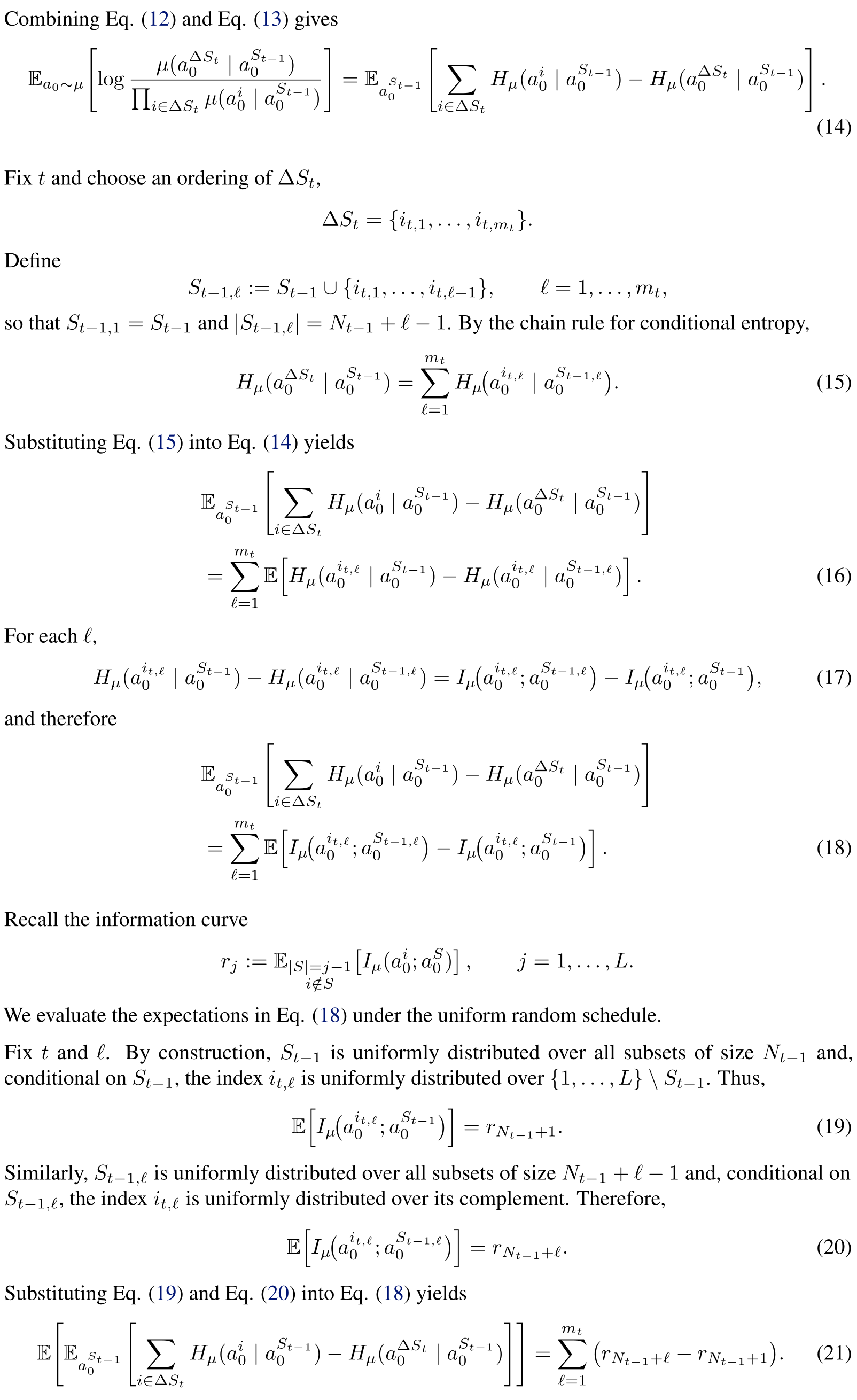
Combining Eq. (12) and Eq. (13) gives
Ea0↓µ
log
µ(a!St
0
| aSt→1
0
)
i↑!St µ(ai
0 | aSt→1
0
)
= Ea
St→1
0
(
i↑!St
Hµ(ai
0 | aSt→1
0
) ↔Hµ(a!St
0
| aSt→1
0
)
.
(14)
Fix t and choose an ordering of !St,
!St = {it,1, . . . , it,mt}.
Define
St→1,ϑ := St→1 ⇑{it,1, . . . , it,ϑ→1},
ϑ = 1, . . . , mt,
so that St→1,1 = St→1 and |St→1,ϑ| = Nt→1 + ϑ ↔1. By the chain rule for conditional entropy,
Hµ(a!St
0
| aSt→1
0
) =
mt
(
ϑ=1
Hµ
,
ait,ω
0
| aSt→1,ω
0
-
.
(15)
Substituting Eq. (15) into Eq. (14) yields
Ea
St→1
0
(
i↑!St
Hµ(ai
0 | aSt→1
0
) ↔Hµ(a!St
0
| aSt→1
0
)
=
mt
(
ϑ=1
E
.
Hµ(ait,ω
0
| aSt→1
0
) ↔Hµ(ait,ω
0
| aSt→1,ω
0
)
/
.
(16)
For each ϑ,
Hµ(ait,ω
0
| aSt→1
0
) ↔Hµ(ait,ω
0
| aSt→1,ω
0
) = Iµ
,
ait,ω
0 ; aSt→1,ω
0
-
↔Iµ
,
ait,ω
0 ; aSt→1
0
-
,
(17)
and therefore
Ea
St→1
0
(
i↑!St
Hµ(ai
0 | aSt→1
0
) ↔Hµ(a!St
0
| aSt→1
0
)
=
mt
(
ϑ=1
E
.
Iµ
,
ait,ω
0 ; aSt→1,ω
0
-
↔Iµ
,
ait,ω
0 ; aSt→1
0
-/
.
(18)
Recall the information curve
rj := E|S|=j→1
i/↑S
&
Iµ(ai
0; aS
0 )
'
,
j = 1, . . . , L.
We evaluate the expectations in Eq. (18) under the uniform random schedule.
Fix t and ϑ. By construction, St→1 is uniformly distributed over all subsets of size Nt→1 and,
conditional on St→1, the index it,ϑ is uniformly distributed over {1, . . . , L} \ St→1. Thus,
E
.
Iµ
,
ait,ω
0 ; aSt→1
0
-/
= rNt→1+1.
(19)
Similarly, St→1,ϑ is uniformly distributed over all subsets of size Nt→1 + ϑ ↔1 and, conditional on
St→1,ϑ, the index it,ϑ is uniformly distributed over its complement. Therefore,
E
.
Iµ
,
ait,ω
0 ; aSt→1,ω
0
-/
= rNt→1+ϑ.
(20)
Substituting Eq. (19) and Eq. (20) into Eq. (18) yields
E
Ea
St→1
0
(
i↑!St
Hµ(ai
0 | aSt→1
0
) ↔Hµ(a!St
0
| aSt→1
0
)
=
mt
(
ϑ=1
,
rNt→1+ϑ ↔rNt→1+1
-
.
(21)
Selectable PDF text; mathematical layout is preserved above
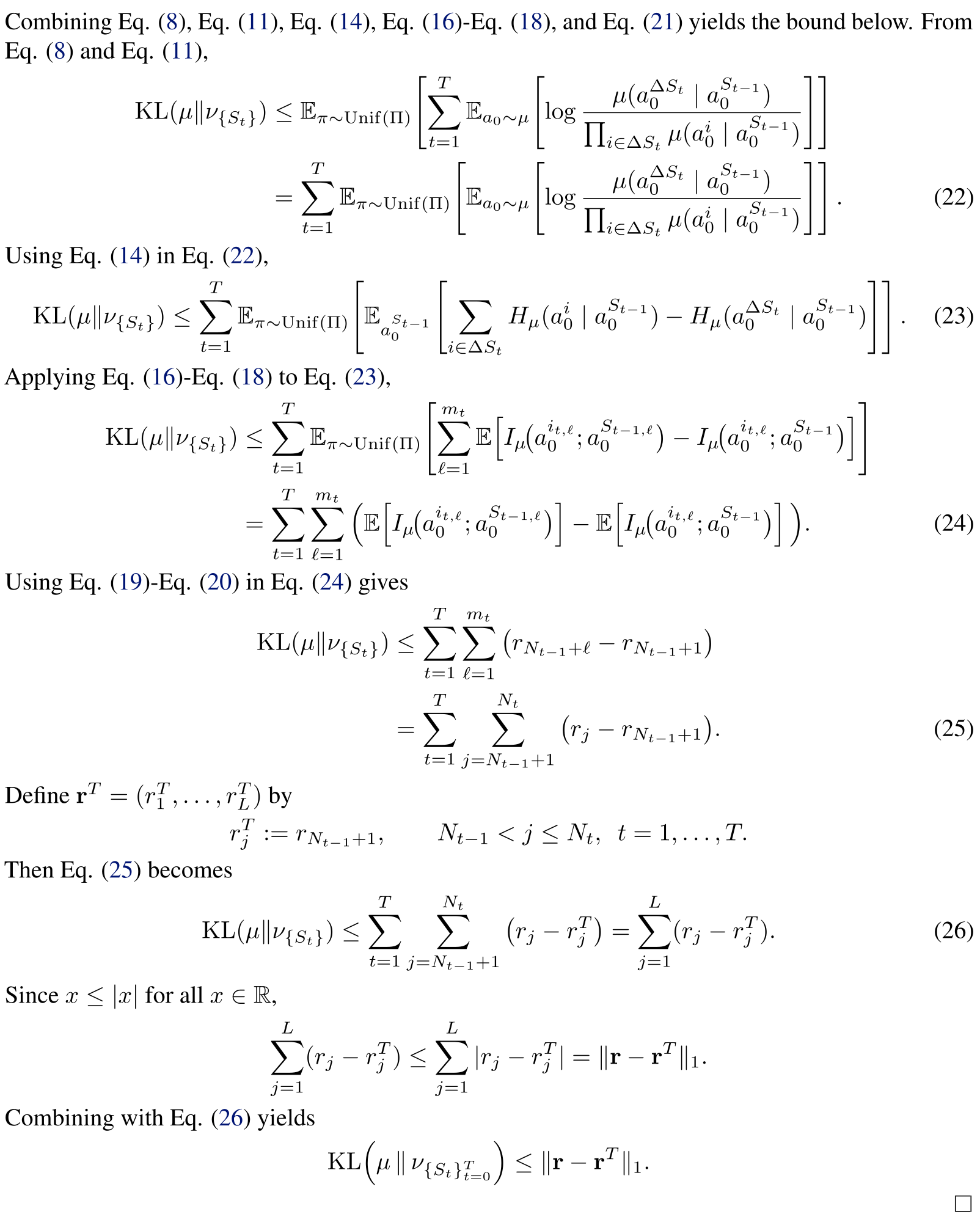
Combining Eq. (8), Eq. (11), Eq. (14), Eq. (16)-Eq. (18), and Eq. (21) yields the bound below. From
Eq. (8) and Eq. (11),
KL(µ↑ω{St}) ↓Eω↓Unif(”)
T
(
t=1
Ea0↓µ
log
µ(a!St
0
| aSt→1
0
)
i↑!St µ(ai
0 | aSt→1
0
)
=
T
(
t=1
Eω↓Unif(”)
Ea0↓µ
log
µ(a!St
0
| aSt→1
0
)
i↑!St µ(ai
0 | aSt→1
0
)
.
(22)
Using Eq. (14) in Eq. (22),
KL(µ↑ω{St}) ↓
T
(
t=1
Eω↓Unif(”)
Ea
St→1
0
(
i↑!St
Hµ(ai
0 | aSt→1
0
) ↔Hµ(a!St
0
| aSt→1
0
)
.
(23)
Applying Eq. (16)-Eq. (18) to Eq. (23),
KL(µ↑ω{St}) ↓
T
(
t=1
Eω↓Unif(”)
mt
(
ϑ=1
E
.
Iµ
,
ait,ω
0 ; aSt→1,ω
0
-
↔Iµ
,
ait,ω
0 ; aSt→1
0
-/
=
T
(
t=1
mt
(
ϑ=1
!
E
.
Iµ
,
ait,ω
0 ; aSt→1,ω
0
-/
↔E
.
Iµ
,
ait,ω
0 ; aSt→1
0
-/ "
.
(24)
Using Eq. (19)-Eq. (20) in Eq. (24) gives
KL(µ↑ω{St}) ↓
T
(
t=1
mt
(
ϑ=1
,
rNt→1+ϑ ↔rNt→1+1
-
=
T
(
t=1
Nt
(
j=Nt→1+1
,
rj ↔rNt→1+1
-
.
(25)
Define rT = (rT
1 , . . . , rT
L) by
rT
j := rNt→1+1,
Nt→1 < j ↓Nt, t = 1, . . . , T.
Then Eq. (25) becomes
KL(µ↑ω{St}) ↓
T
(
t=1
Nt
(
j=Nt→1+1
,
rj ↔rT
j
-
=
L
(
j=1
(rj ↔rT
j ).
(26)
Since x ↓|x| for all x ↖R,
L
(
j=1
(rj ↔rT
j ) ↓
L
(
j=1
|rj ↔rT
j | = ↑r ↔rT ↑1.
Combining with Eq. (26) yields
KL
!
µ ↑ω{St}T
t=0
"
↓↑r ↔rT ↑1.
Appendix B.2 · Conditioning theorem
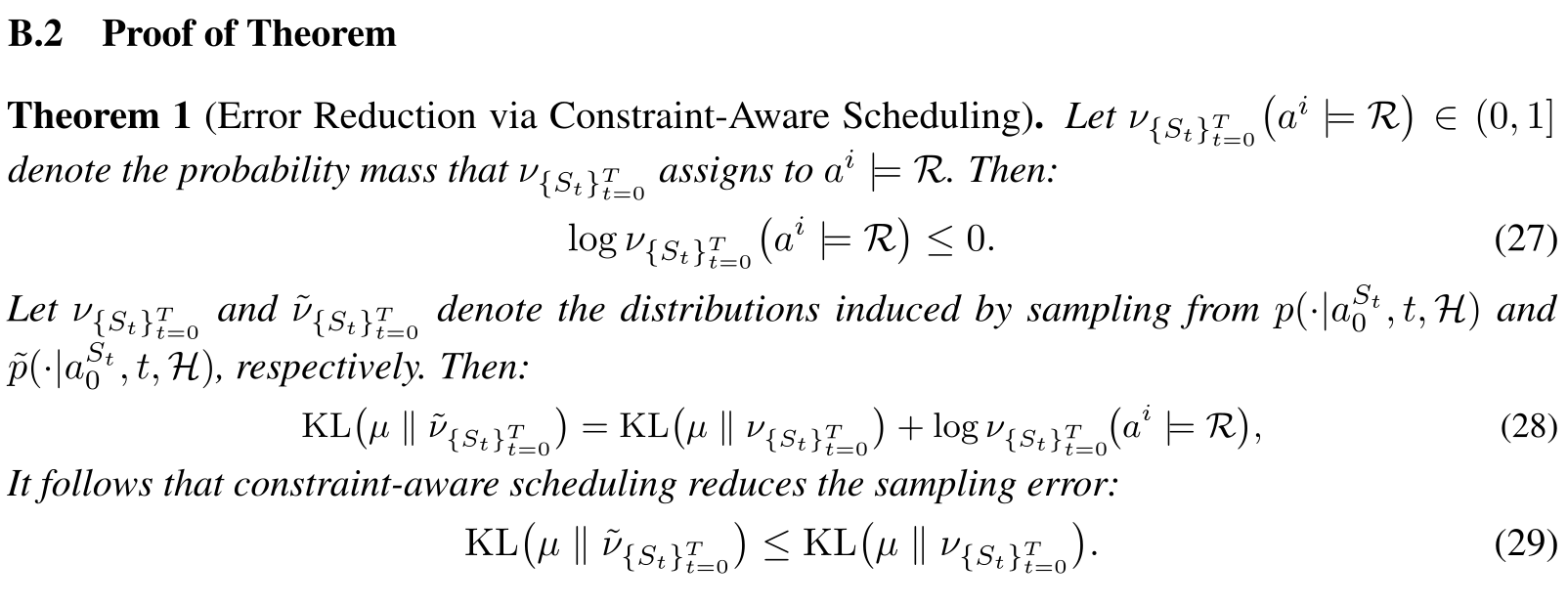
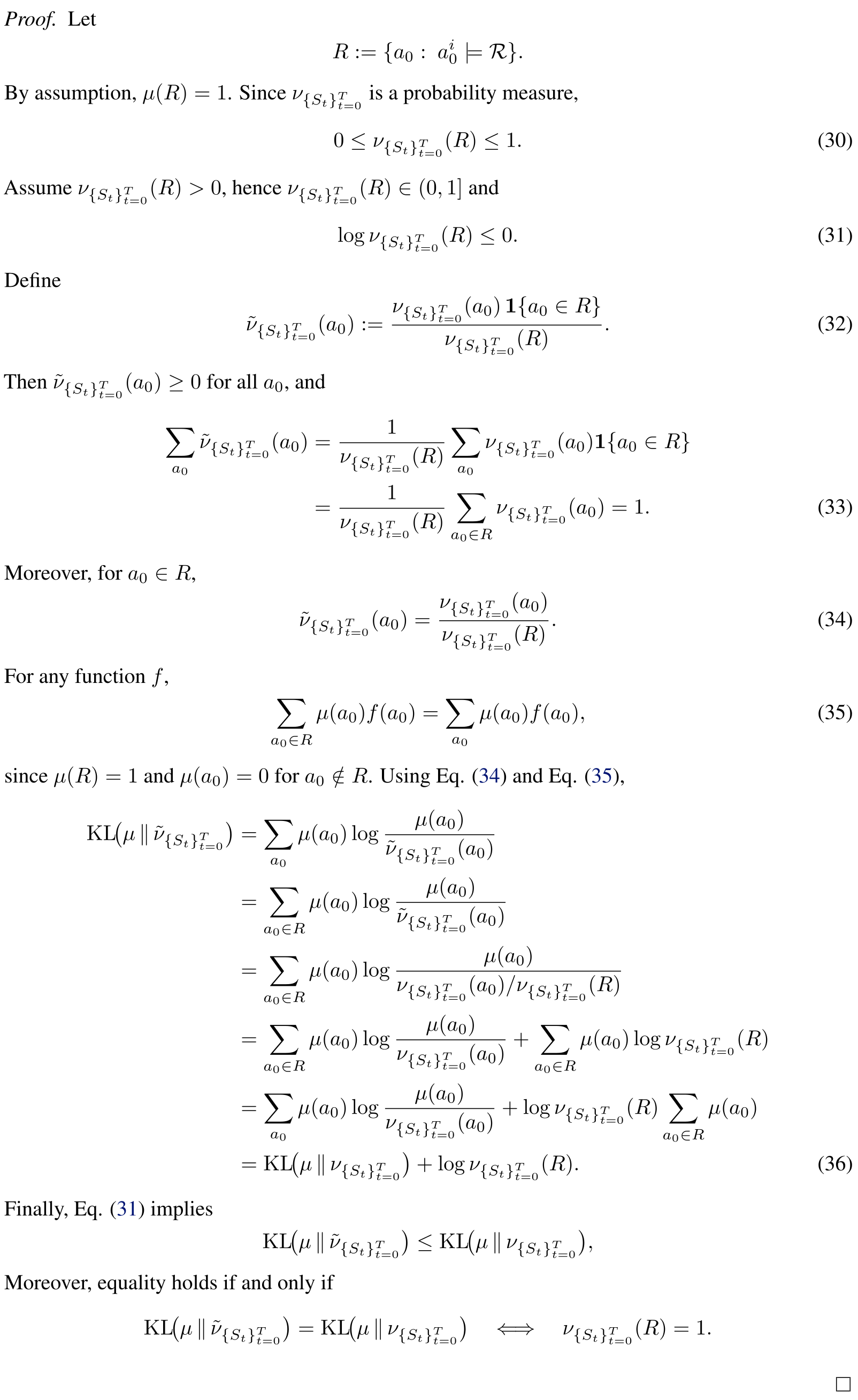
The theorem defines a feasible joint-sequence set with full data-distribution support, requires positive base probability on that set, and explicitly constructs the constrained joint law by dividing by one global feasible-set probability. Under that definition the KL change is exactly the logarithm of that probability, hence nonpositive. The implemented per-position masking is not shown to produce this same law. For example, base probabilities (00,01,10,11)=(.1,.4,.4,.1) and feasible set {00,10,11} give global conditioning (1/6,2/3,1/6), whereas revealing the first token before masking the second gives (.5,.4,.1). This illustrates the missing equivalence step, not evidence that the reported code fails its tests. The full theorem and proof remain unchanged.
Selectable PDF text; mathematical layout is preserved above
B.2
Proof of Theorem
Theorem 1 (Error Reduction via Constraint-Aware Scheduling). Let ω{St}T
t=0
,
ai |= R
-
↖(0, 1]
denote the probability mass that ω{St}T
t=0 assigns to ai |= R. Then:
log ω{St}T
t=0
,
ai |= R
-
↓0.
(27)
Let ω{St}T
t=0 and ˜ω{St}T
t=0 denote the distributions induced by sampling from p(·|aSt
0 , t, H) and
˜p(·|aSt
0 , t, H), respectively. Then:
KL
"
µ ↓˜ω{St}T
t=0
#
= KL
"
µ ↓ω{St}T
t=0
#
+ log ω{St}T
t=0
"
ai |= R
#
,
(28)
It follows that constraint-aware scheduling reduces the sampling error:
KL
,
µ ↑˜ω{St}T
t=0
-
↓KL
,
µ ↑ω{St}T
t=0
-
.
(29)
Selectable PDF text; mathematical layout is preserved above
Proof. Let
R := {a0 : ai
0 |= R}.
By assumption, µ(R) = 1. Since ω{St}T
t=0 is a probability measure,
0 ↓ω{St}T
t=0(R) ↓1.
(30)
Assume ω{St}T
t=0(R) > 0, hence ω{St}T
t=0(R) ↖(0, 1] and
log ω{St}T
t=0(R) ↓0.
(31)
Define
˜ω{St}T
t=0(a0) :=
ω{St}T
t=0(a0) 1{a0 ↖R}
ω{St}T
t=0(R)
.
(32)
Then ˜ω{St}T
t=0(a0) ⇐0 for all a0, and
(
a0
˜ω{St}T
t=0(a0) =
1
ω{St}T
t=0(R)
(
a0
ω{St}T
t=0(a0)1{a0 ↖R}
=
1
ω{St}T
t=0(R)
(
a0↑R
ω{St}T
t=0(a0) = 1.
(33)
Moreover, for a0 ↖R,
˜ω{St}T
t=0(a0) =
ω{St}T
t=0(a0)
ω{St}T
t=0(R) .
(34)
For any function f,
(
a0↑R
µ(a0)f(a0) =
(
a0
µ(a0)f(a0),
(35)
since µ(R) = 1 and µ(a0) = 0 for a0 /↖R. Using Eq. (34) and Eq. (35),
KL
,
µ ↑˜ω{St}T
t=0
-
=
(
a0
µ(a0) log
µ(a0)
˜ω{St}T
t=0(a0)
=
(
a0↑R
µ(a0) log
µ(a0)
˜ω{St}T
t=0(a0)
=
(
a0↑R
µ(a0) log
µ(a0)
ω{St}T
t=0(a0)/ω{St}T
t=0(R)
=
(
a0↑R
µ(a0) log
µ(a0)
ω{St}T
t=0(a0) +
(
a0↑R
µ(a0) log ω{St}T
t=0(R)
=
(
a0
µ(a0) log
µ(a0)
ω{St}T
t=0(a0) + log ω{St}T
t=0(R)
(
a0↑R
µ(a0)
= KL
,
µ ↑ω{St}T
t=0
-
+ log ω{St}T
t=0(R).
(36)
Finally, Eq. (31) implies
KL
,
µ ↑˜ω{St}T
t=0
-
↓KL
,
µ ↑ω{St}T
t=0
-
,
Moreover, equality holds if and only if
KL
,
µ ↑˜ω{St}T
t=0
-
= KL
,
µ ↑ω{St}T
t=0
-
↙∝
ω{St}T
t=0(R) = 1.
Appendix C · Complexity analysis
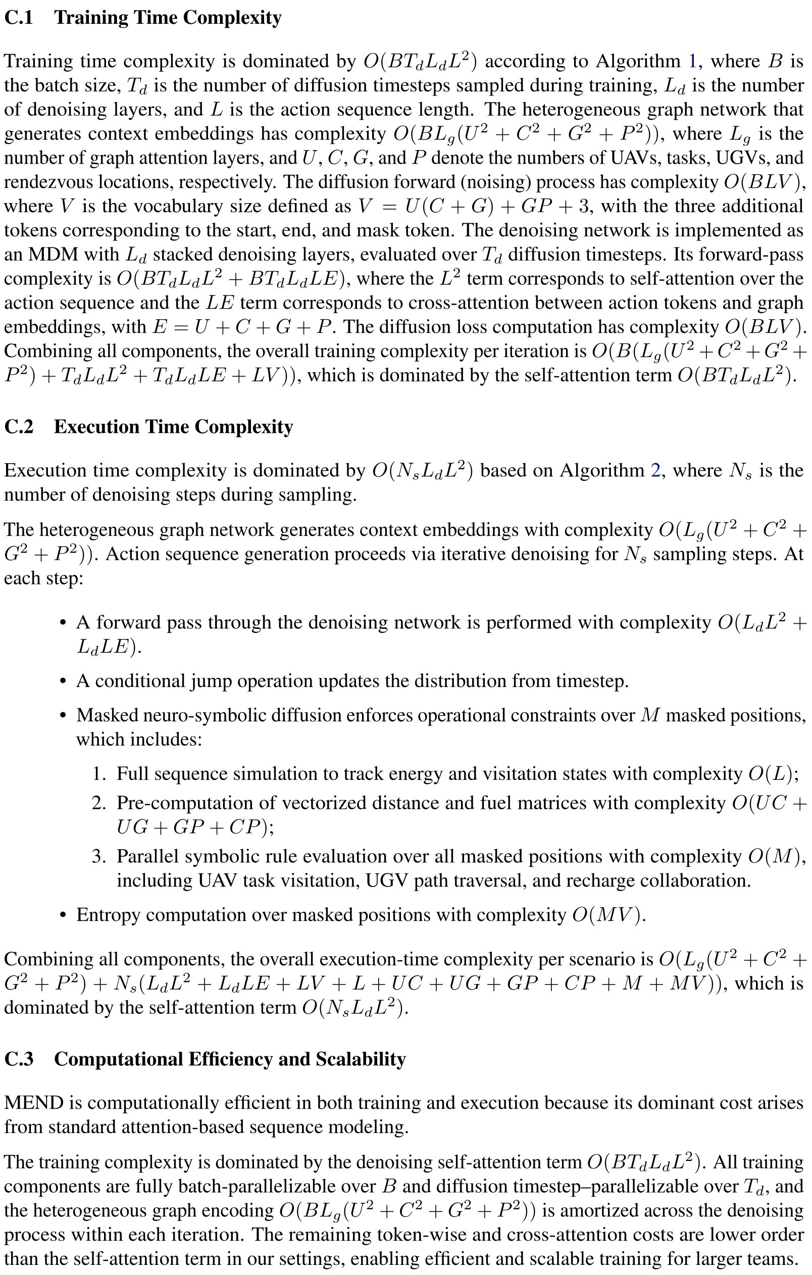
The appendix retains every graph, token, cross-attention, vocabulary, sequence-simulation, fuel-matrix, symbolic-mask and entropy cost term. Its dominant attention costs are quadratic in action length and linear in decoding steps for the stated architecture. Rule evaluation is specialized vectorized tensor code, not general-purpose FOL reasoning. Additional rules affect constant factors only under the assumed fixed rule structure and entity dimensions; the analysis does not establish constant cost for arbitrary logical programs or unlimited new constraints.
Selectable PDF text; mathematical layout is preserved above
C.1
Training Time Complexity
Training time complexity is dominated by O(BTdLdL2) according to Algorithm 1, where B is
the batch size, Td is the number of diffusion timesteps sampled during training, Ld is the number
of denoising layers, and L is the action sequence length. The heterogeneous graph network that
generates context embeddings has complexity O(BLg(U 2 + C2 + G2 + P 2)), where Lg is the
number of graph attention layers, and U, C, G, and P denote the numbers of UAVs, tasks, UGVs, and
rendezvous locations, respectively. The diffusion forward (noising) process has complexity O(BLV ),
where V is the vocabulary size defined as V = U(C + G) + GP + 3, with the three additional
tokens corresponding to the start, end, and mask token. The denoising network is implemented as
an MDM with Ld stacked denoising layers, evaluated over Td diffusion timesteps. Its forward-pass
complexity is O(BTdLdL2 + BTdLdLE), where the L2 term corresponds to self-attention over the
action sequence and the LE term corresponds to cross-attention between action tokens and graph
embeddings, with E = U + C + G + P. The diffusion loss computation has complexity O(BLV ).
Combining all components, the overall training complexity per iteration is O(B(Lg(U 2 + C2 + G2 +
P 2) + TdLdL2 + TdLdLE + LV )), which is dominated by the self-attention term O(BTdLdL2).
C.2
Execution Time Complexity
Execution time complexity is dominated by O(NsLdL2) based on Algorithm 2, where Ns is the
number of denoising steps during sampling.
The heterogeneous graph network generates context embeddings with complexity O(Lg(U 2 + C2 +
G2 + P 2)). Action sequence generation proceeds via iterative denoising for Ns sampling steps. At
each step:
• A forward pass through the denoising network is performed with complexity O(LdL2 +
LdLE).
• A conditional jump operation updates the distribution from timestep.
• Masked neuro-symbolic diffusion enforces operational constraints over M masked positions,
which includes:
1. Full sequence simulation to track energy and visitation states with complexity O(L);
2. Pre-computation of vectorized distance and fuel matrices with complexity O(UC +
UG + GP + CP);
3. Parallel symbolic rule evaluation over all masked positions with complexity O(M),
including UAV task visitation, UGV path traversal, and recharge collaboration.
• Entropy computation over masked positions with complexity O(MV ).
Combining all components, the overall execution-time complexity per scenario is O(Lg(U 2 + C2 +
G2 + P 2) + Ns(LdL2 + LdLE + LV + L + UC + UG + GP + CP + M + MV )), which is
dominated by the self-attention term O(NsLdL2).
C.3
Computational Efficiency and Scalability
MEND is computationally efficient in both training and execution because its dominant cost arises
from standard attention-based sequence modeling.
The training complexity is dominated by the denoising self-attention term O(BTdLdL2). All training
components are fully batch-parallelizable over B and diffusion timestep–parallelizable over Td, and
the heterogeneous graph encoding O(BLg(U 2 + C2 + G2 + P 2)) is amortized across the denoising
process within each iteration. The remaining token-wise and cross-attention costs are lower order
than the self-attention term in our settings, enabling efficient and scalable training for larger teams.
Selectable PDF text; mathematical layout is preserved above
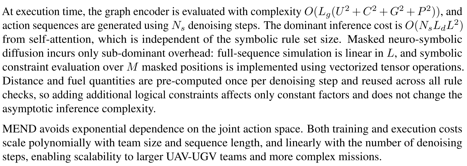
At execution time, the graph encoder is evaluated with complexity O(Lg(U 2 + C2 + G2 + P 2)), and
action sequences are generated using Ns denoising steps. The dominant inference cost is O(NsLdL2)
from self-attention, which is independent of the symbolic rule set size. Masked neuro-symbolic
diffusion incurs only sub-dominant overhead: full-sequence simulation is linear in L, and symbolic
constraint evaluation over M masked positions is implemented using vectorized tensor operations.
Distance and fuel quantities are pre-computed once per denoising step and reused across all rule
checks, so adding additional logical constraints affects only constant factors and does not change the
asymptotic inference complexity.
MEND avoids exponential dependence on the joint action space. Both training and execution costs
scale polynomially with team size and sequence length, and linearly with the number of denoising
steps, enabling scalability to larger UAV-UGV teams and more complex missions.
Appendix D.1–D.2 · Vectorized symbolic rules
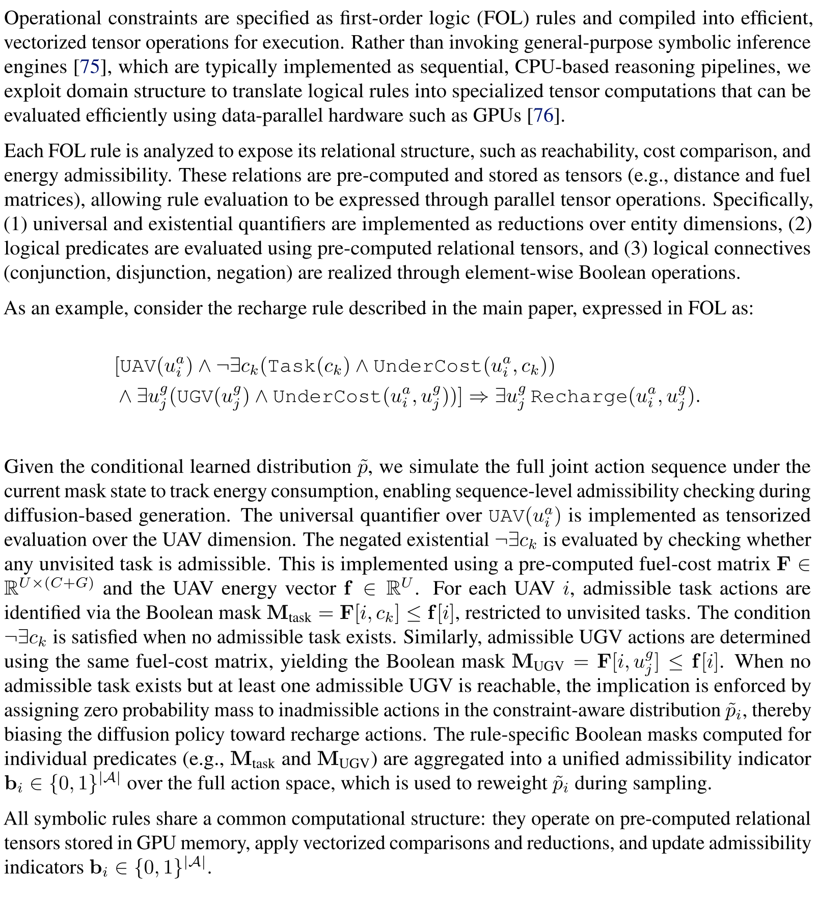
Quantifiers become reductions over entity dimensions, predicates use precomputed distance/fuel tensors, and connectives become Boolean operations. Full-sequence simulation tracks energy and visitation under the current mask state. When no affordable unvisited task exists but a UGV is affordable, inadmissible actions are zeroed to favor recharge. The three example rules and full tensor implementation remain. The text does not completely specify how unresolved masked actions are instantiated for every simulated history or what happens when no admissible probability survives.
Selectable PDF text; mathematical layout is preserved above
Operational constraints are specified as first-order logic (FOL) rules and compiled into efficient,
vectorized tensor operations for execution. Rather than invoking general-purpose symbolic inference
engines [75], which are typically implemented as sequential, CPU-based reasoning pipelines, we
exploit domain structure to translate logical rules into specialized tensor computations that can be
evaluated efficiently using data-parallel hardware such as GPUs [76].
Each FOL rule is analyzed to expose its relational structure, such as reachability, cost comparison, and
energy admissibility. These relations are pre-computed and stored as tensors (e.g., distance and fuel
matrices), allowing rule evaluation to be expressed through parallel tensor operations. Specifically,
(1) universal and existential quantifiers are implemented as reductions over entity dimensions, (2)
logical predicates are evaluated using pre-computed relational tensors, and (3) logical connectives
(conjunction, disjunction, negation) are realized through element-wise Boolean operations.
As an example, consider the recharge rule described in the main paper, expressed in FOL as:
[UAV(ua
i ) ′ ¬∞ck(Task(ck) ′ UnderCost(ua
i , ck))
′ ∞ug
j(UGV(ug
j) ′ UnderCost(ua
i , ug
j))] ∝∞ug
j Recharge(ua
i , ug
j).
Given the conditional learned distribution ˜p, we simulate the full joint action sequence under the
current mask state to track energy consumption, enabling sequence-level admissibility checking during
diffusion-based generation. The universal quantifier over UAV(ua
i ) is implemented as tensorized
evaluation over the UAV dimension. The negated existential °ck is evaluated by checking whether
any unvisited task is admissible. This is implemented using a pre-computed fuel-cost matrix F ↖
RU↗(C+G) and the UAV energy vector f ↖RU. For each UAV i, admissible task actions are
identified via the Boolean mask Mtask = F[i, ck] ↓f[i], restricted to unvisited tasks. The condition
°ck is satisfied when no admissible task exists. Similarly, admissible UGV actions are determined
using the same fuel-cost matrix, yielding the Boolean mask MUGV = F[i, ug
j] ↓f[i]. When no
admissible task exists but at least one admissible UGV is reachable, the implication is enforced by
assigning zero probability mass to inadmissible actions in the constraint-aware distribution ˜pi, thereby
biasing the diffusion policy toward recharge actions. The rule-specific Boolean masks computed for
individual predicates (e.g., Mtask and MUGV) are aggregated into a unified admissibility indicator
bi ↖{0, 1}|A| over the full action space, which is used to reweight ˜pi during sampling.
All symbolic rules share a common computational structure: they operate on pre-computed relational
tensors stored in GPU memory, apply vectorized comparisons and reductions, and update admissibility
indicators bi ↖{0, 1}|A|.
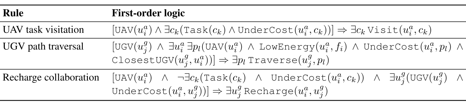
Selectable PDF text; mathematical layout is preserved above
Rule First-order logic UAV task visitation [UAV(ua i ) ′ ∞ck(Task(ck) ′ UnderCost(ua i , ck))] ∝∞ck Visit(ua i , ck) UGV path traversal [UGV(ug j) ′ ∞ua i ∞pl(UAV(ua i ) ′ LowEnergy(ua i , fi) ′ UnderCost(ua i , pl) ′ ClosestUGV(ug j, ua i ))] ∝∞pl Traverse(ug j, pl) Recharge collaboration [UAV(ua i ) ′ ¬∞ck(Task(ck) ′ UnderCost(ua i , ck)) ′ ∞ug j(UGV(ug j) ′ UnderCost(ua i , ug j))] ∝∞ug j Recharge(ua i , ug j)
Appendix D.3 · Model architecture
The graph encoder has two eight-head layers with 128-dimensional embeddings. The denoiser has four Transformer layers, eight heads and feedforward width 512, with 128-dimensional token/timestep embeddings and positional embeddings up to length 1000. A cosine absorbing-mask schedule uses 1000 training timesteps, offset .008 and twenty inference denoising steps. The exact source formula remains; the manuscript does not fully reconcile twenty inference steps with pseudocode that reveals one position per loop and iterates T down to one for variable sequence lengths.

Selectable PDF text; mathematical layout is preserved above
Diffusion process. We adopt a discrete absorbing diffusion process with T = 1000 timesteps using a
cosine noise schedule with offset parameter s = 0.008. The forward masking process is defined by
ϖt = cos
, ω
2 (t/T + s)/(1 + s)
-
/ cos
,
εs/(2(1 + s))
-
. At inference time, the MDMs enable parallel
token unmasking, providing an efficient decoding mechanism. We use 20 denoising steps to gradually
reveal action sequences from an initially fully masked state.
Appendix D.4 · Hyperparameters
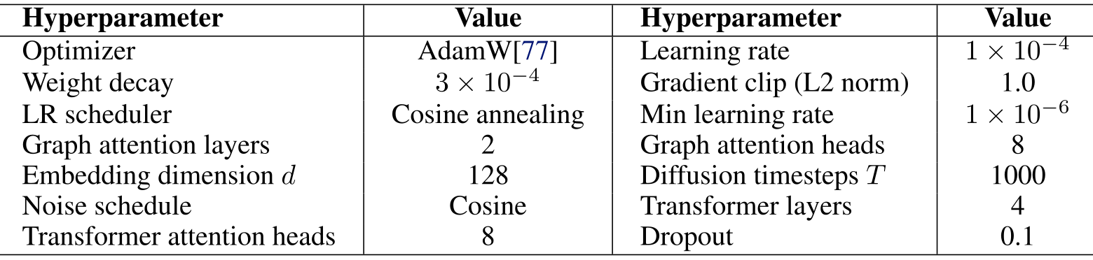
AdamW uses learning rate 1e-4, weight decay 3e-4, gradient-norm clipping at 1, cosine annealing to 1e-6 and dropout .1. The retained table gives the complete reported configuration. Experiments use a 16-core Intel i9, 32 GB RAM and an RTX 4090. Epoch counts, batch size and independent training-seed counts are not provided here.
Selectable PDF text; mathematical layout is preserved above
Hyperparameter
Value
Hyperparameter
Value
Optimizer
AdamW[77]
Learning rate
1 ∈10→4
Weight decay
3 ∈10→4
Gradient clip (L2 norm)
1.0
LR scheduler
Cosine annealing
Min learning rate
1 ∈10→6
Graph attention layers
2
Graph attention heads
8
Embedding dimension d
128
Diffusion timesteps T
1000
Noise schedule
Cosine
Transformer layers
4
Transformer attention heads
8
Dropout
0.1
Appendix E.1 · Mixed-integer expert formulation
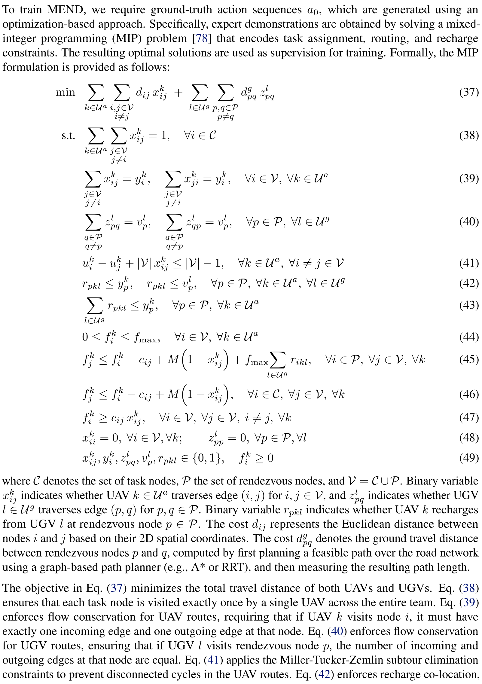
Gurobi produces expert sequences from a mixed-integer route/recharge problem. The stated objective minimizes total aerial and ground travel distance. Constraints assign every task once, conserve flow, suppress UAV subtours, couple recharge to co-located visits and track UAV energy. All thirteen numbered constraints/objective, variable definitions and their explanations remain. Makespan synchronization and UGV energy limits are not fully specified in the displayed formulation, so it should not be treated as a complete independent certificate for every claimed operational constraint or each evaluation metric.
Selectable PDF text; mathematical layout is preserved above
To train MEND, we require ground-truth action sequences a0, which are generated using an
optimization-based approach. Specifically, expert demonstrations are obtained by solving a mixed-
integer programming (MIP) problem [78] that encodes task assignment, routing, and recharge
constraints. The resulting optimal solutions are used as supervision for training. Formally, the MIP
formulation is provided as follows:
min
(
k↑Ua
(
i,j↑V
i↘=j
dij xk
ij +
(
l↑Ug
(
p,q↑P
p↘=q
dg
pq zl
pq
(37)
s.t.
(
k↑Ua
(
j↑V
j↘=i
xk
ij = 1,
↘i ↖C
(38)
(
j↑V
j↘=i
xk
ij = yk
i ,
(
j↑V
j↘=i
xk
ji = yk
i ,
↘i ↖V, ↘k ↖Ua
(39)
(
q↑P
q↘=p
zl
pq = vl
p,
(
q↑P
q↘=p
zl
qp = vl
p,
↘p ↖P, ↘l ↖Ug
(40)
uk
i ↔uk
j + |V| xk
ij ↓|V| ↔1,
↘k ↖Ua, ↘i →= j ↖V
(41)
rpkl ↓yk
p,
rpkl ↓vl
p,
↘p ↖P, ↘k ↖Ua, ↘l ↖Ug
(42)
(
l↑Ug
rpkl ↓yk
p,
↘p ↖P, ↘k ↖Ua
(43)
0 ↓f k
i ↓fmax,
↘i ↖V, ↘k ↖Ua
(44)
f k
j ↓f k
i ↔cij + M
!
1 ↔xk
ij
"
+ fmax
(
l↑Ug
rikl,
↘i ↖P, ↘j ↖V, ↘k
(45)
f k
j ↓f k
i ↔cij + M
!
1 ↔xk
ij
"
,
↘i ↖C, ↘j ↖V, ↘k
(46)
f k
i ⇐cij xk
ij,
↘i ↖V, ↘j ↖V, i →= j, ↘k
(47)
xk
ii = 0, ↘i ↖V, ↘k;
zl
pp = 0, ↘p ↖P, ↘l
(48)
xk
ij, yk
i , zl
pq, vl
p, rpkl ↖{0, 1},
f k
i ⇐0
(49)
where C denotes the set of task nodes, P the set of rendezvous nodes, and V = C ⇑P. Binary variable
xk
ij indicates whether UAV k ↖Ua traverses edge (i, j) for i, j ↖V, and zl
pq indicates whether UGV
l ↖Ug traverses edge (p, q) for p, q ↖P. Binary variable rpkl indicates whether UAV k recharges
from UGV l at rendezvous node p ↖P. The cost dij represents the Euclidean distance between
nodes i and j based on their 2D spatial coordinates. The cost dg
pq denotes the ground travel distance
between rendezvous nodes p and q, computed by first planning a feasible path over the road network
using a graph-based path planner (e.g., A* or RRT), and then measuring the resulting path length.
The objective in Eq. (37) minimizes the total travel distance of both UAVs and UGVs. Eq. (38)
ensures that each task node is visited exactly once by a single UAV across the entire team. Eq. (39)
enforces flow conservation for UAV routes, requiring that if UAV k visits node i, it must have
exactly one incoming edge and one outgoing edge at that node. Eq. (40) enforces flow conservation
for UGV routes, ensuring that if UGV l visits rendezvous node p, the number of incoming and
outgoing edges at that node are equal. Eq. (41) applies the Miller-Tucker-Zemlin subtour elimination
constraints to prevent disconnected cycles in the UAV routes. Eq. (42) enforces recharge co-location,
Selectable PDF text; mathematical layout is preserved above
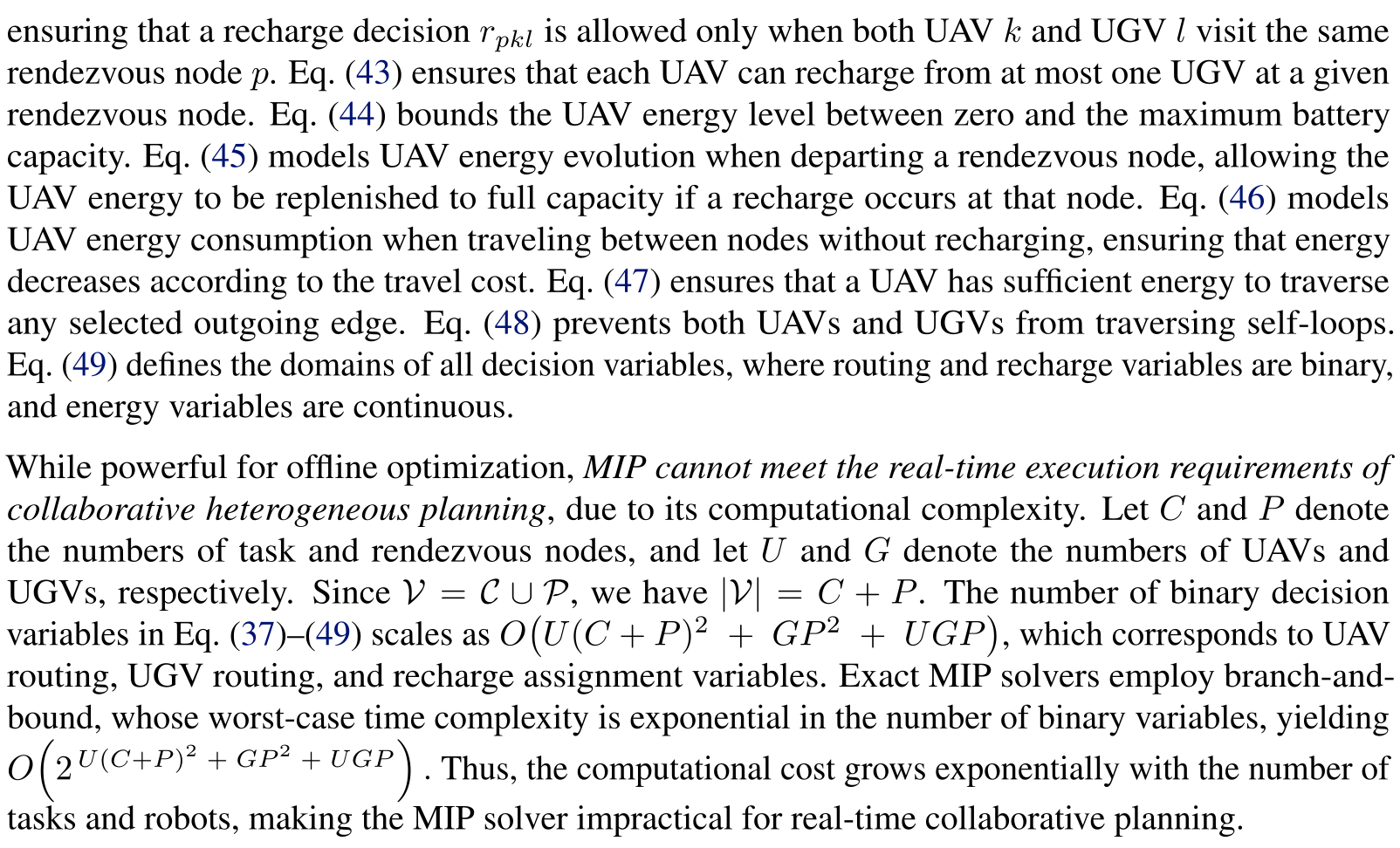
ensuring that a recharge decision rpkl is allowed only when both UAV k and UGV l visit the same
rendezvous node p. Eq. (43) ensures that each UAV can recharge from at most one UGV at a given
rendezvous node. Eq. (44) bounds the UAV energy level between zero and the maximum battery
capacity. Eq. (45) models UAV energy evolution when departing a rendezvous node, allowing the
UAV energy to be replenished to full capacity if a recharge occurs at that node. Eq. (46) models
UAV energy consumption when traveling between nodes without recharging, ensuring that energy
decreases according to the travel cost. Eq. (47) ensures that a UAV has sufficient energy to traverse
any selected outgoing edge. Eq. (48) prevents both UAVs and UGVs from traversing self-loops.
Eq. (49) defines the domains of all decision variables, where routing and recharge variables are binary,
and energy variables are continuous.
While powerful for offline optimization, MIP cannot meet the real-time execution requirements of
collaborative heterogeneous planning, due to its computational complexity. Let C and P denote
the numbers of task and rendezvous nodes, and let U and G denote the numbers of UAVs and
UGVs, respectively. Since V = C ⇑P, we have |V| = C + P. The number of binary decision
variables in Eq. (37)–(49) scales as O
,
U(C + P)2 + GP 2 + UGP
-
, which corresponds to UAV
routing, UGV routing, and recharge assignment variables. Exact MIP solvers employ branch-and-
bound, whose worst-case time complexity is exponential in the number of binary variables, yielding
O
!
2 U(C+P )2 + GP 2 + UGP "
. Thus, the computational cost grows exponentially with the number of
tasks and robots, making the MIP solver impractical for real-time collaborative planning.
Appendix E.2 · Training and dataset
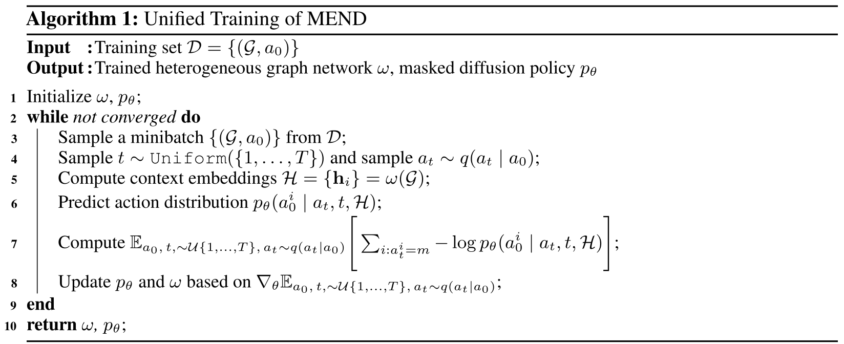
The graph encoder and denoiser train jointly on masked clean-action likelihood. Each dataset contains 1000 randomly generated instances: 800 training and 200 held out for evaluation, varying robot/task/path settings. Algorithm 1 retains all sampling, forward prediction, loss and gradient steps. The paper does not state how many independent dataset/training repetitions underlie each mean or give the final successful-intersection denominator used for conditional metrics.
Selectable PDF text; mathematical layout is preserved above
Algorithm 1: Unified Training of MEND
Input
:Training set D = {(G, a0)}
Output :Trained heterogeneous graph network ε, masked diffusion policy pω
1 Initialize ε, pω;
2 while not converged do
3
Sample a minibatch {(G, a0)} from D;
4
Sample t ↔Uniform({1, . . . , T}) and sample at ↔q(at | a0);
5
Compute context embeddings H = {hi} = ε(G);
6
Predict action distribution pω(ai
0 | at, t, H);
7
Compute Ea0, t,↔U{1,...,T }, at↔q(at|a0)
$
%
i:ai
t=m ↑log pω(ai
0 | at, t, H)
&
;
8
Update pω and ε based on ↗ωEa0, t,↔U{1,...,T }, at↔q(at|a0);
9 end
10 return ε, pω;
Appendix E.3 · Execution procedure
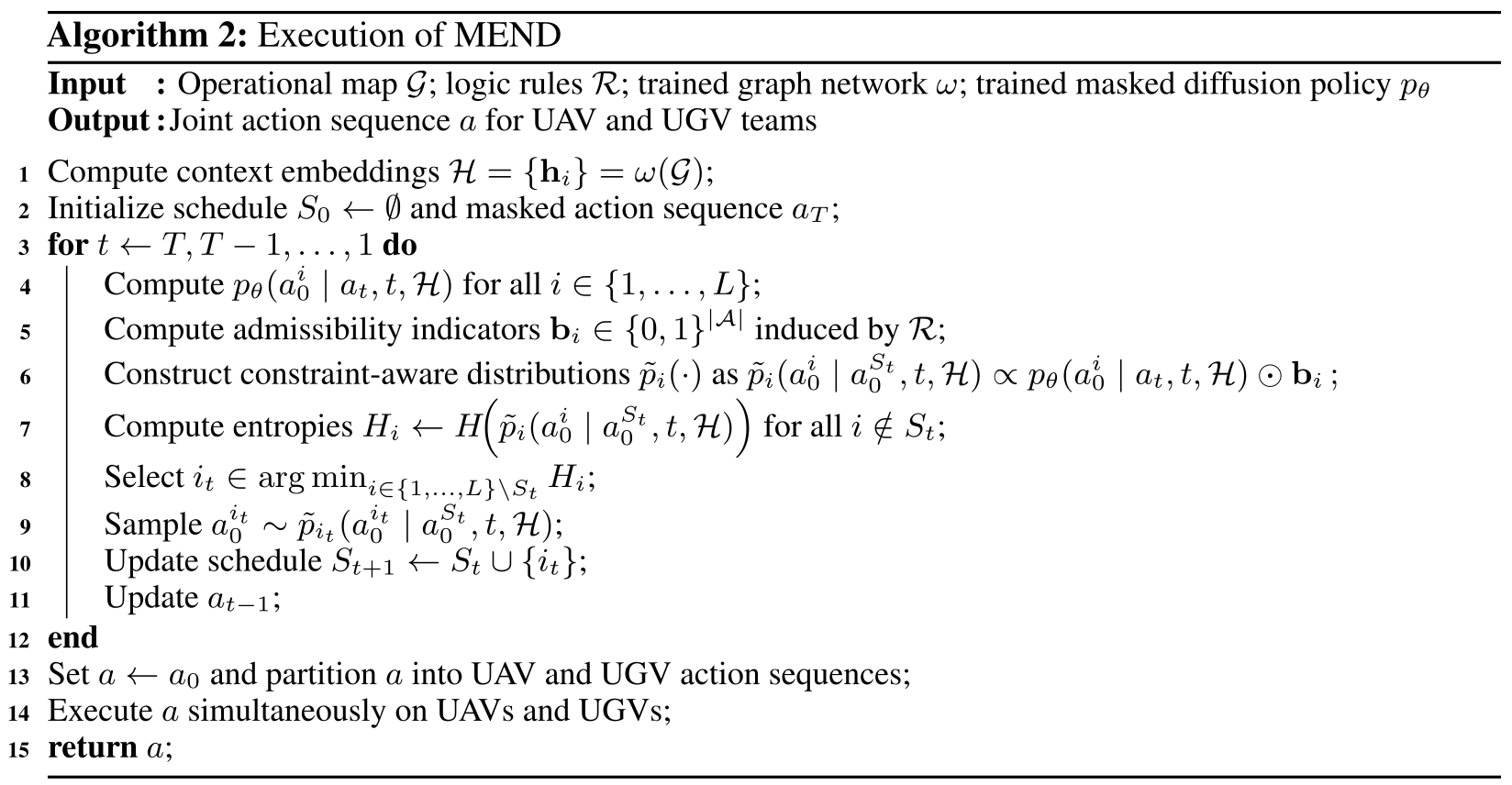
Algorithm 2 encodes the map, initializes a fully masked sequence, predicts each token distribution, constructs rule masks, computes constrained entropies, samples a minimum-entropy position, updates the sequence and finally partitions/executed actions across robots. Its complete original line numbering and formulas remain. The pseudocode mixes descending diffusion t with growing S(t+1) and leaves the inference-step/sequence-length mapping to the description; the edition preserves it without inventing a corrected algorithm.
Selectable PDF text; mathematical layout is preserved above
Algorithm 2: Execution of MEND
Input
: Operational map G; logic rules R; trained graph network ε; trained masked diffusion policy pω
Output :Joint action sequence a for UAV and UGV teams
1 Compute context embeddings H = {hi} = ε(G);
2 Initialize schedule S0 ↘≃and masked action sequence aT ;
3 for t ↘T, T ↑1, . . . , 1 do
4
Compute pω(ai
0 | at, t, H) for all i ⇐{1, . . . , L};
5
Compute admissibility indicators bi ⇐{0, 1}|A| induced by R;
6
Construct constraint-aware distributions ˜pi(·) as ˜pi(ai
0 | aSt
0 , t, H) ⇒pω(ai
0 | at, t, H) ⇑bi ;
7
Compute entropies Hi ↘H
'
˜pi(ai
0 | aSt
0 , t, H)
(
for all i /⇐St;
8
Select it ⇐arg mini↓{1,...,L}\St Hi;
9
Sample ait
0 ↔˜pit(ait
0 | aSt
0 , t, H);
10
Update schedule St+1 ↘St →{it};
11
Update at→1;
12 end
13 Set a ↘a0 and partition a into UAV and UGV action sequences;
14 Execute a simultaneously on UAVs and UGVs;
15 return a;
Appendix F.1 · Mixed-integer comparison
The full largest-mission MIP comparison preserves all reported values. The inference advantage is substantial on this tested configuration, with small reported objective gaps. The displayed distance-minimizing expert program does not establish a theoretical approximation ratio for makespan or energy, and the measured hardware/problem instance matters for timing.

Selectable PDF text; mathematical layout is preserved above
Mission
Method
Makespan
Energy
Speed
T45–P10
4UAV–2UGV
MIP
4369.18
11433.37
0.006 Hz
MEND
4555.97
12114.19
2.830 Hz
Appendix F.2 · Rural generalization
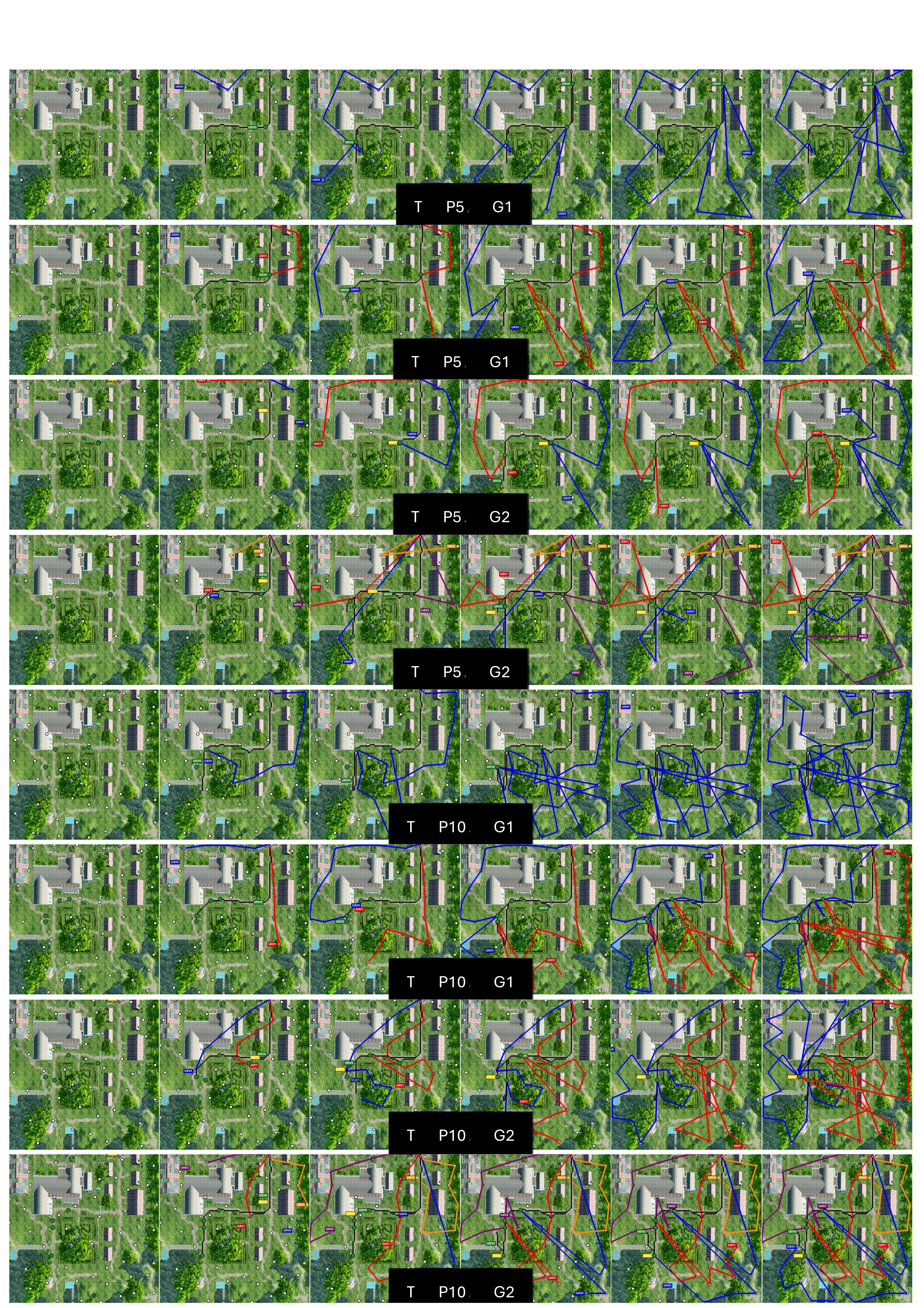
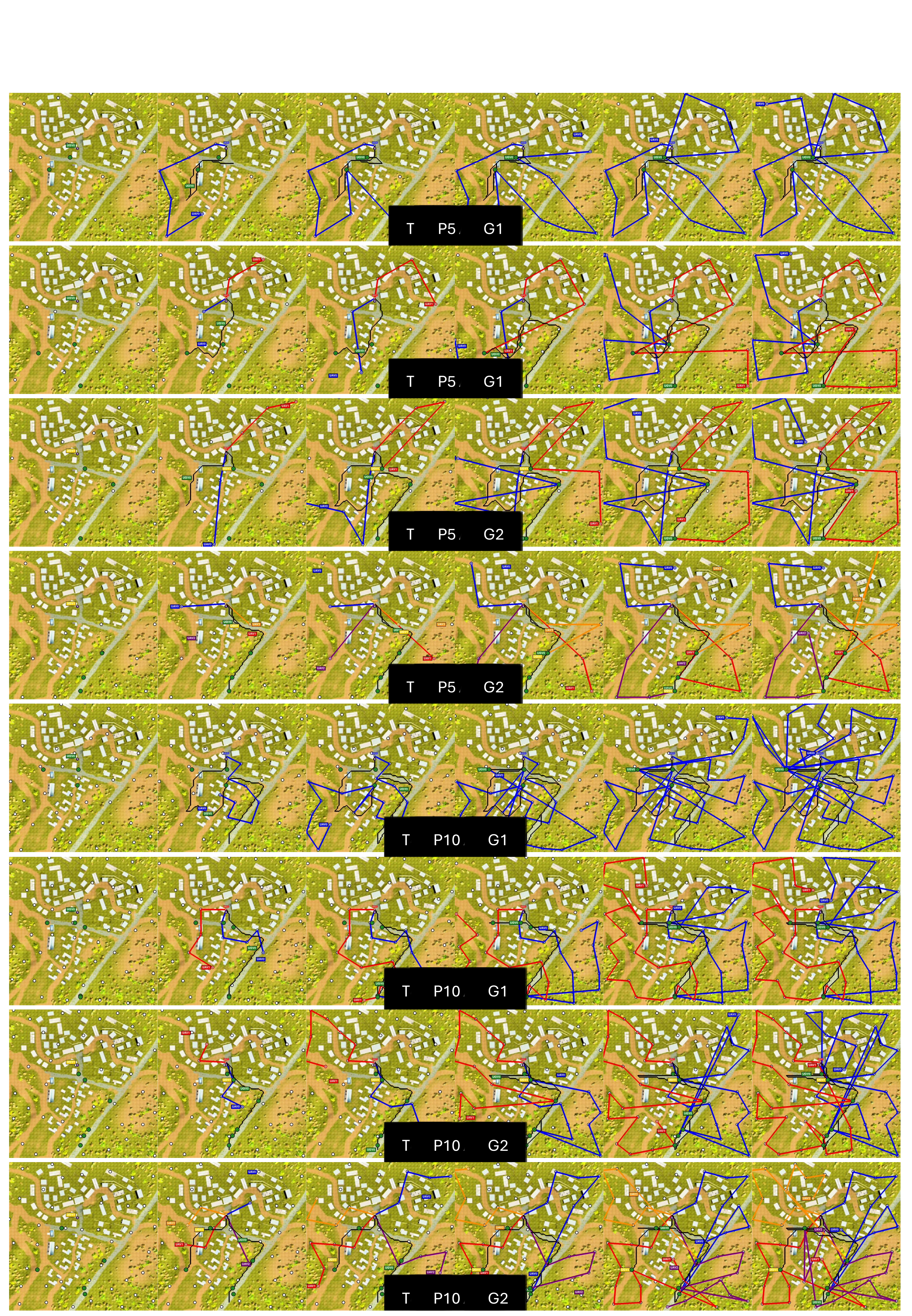
All eight rural montage rows remain: two workloads crossed with four teams, using the training map/roads but newly sampled task positions. Their many time panels show coordination and recharge events. These are selected qualitative scenarios, separate from the aggregate test metrics.
Selectable PDF text; mathematical layout is preserved above
T15-P5 A1-G1
T15-P5 A2-G1
T15-P5 A2-G2
T15-P5 A4-G2
T45-P10 A1-G1
T45-P10 A2-G1
T45-P10 A2-G2
T45-P10 A4-G2
Appendix F.3 · Unseen city and suburban maps
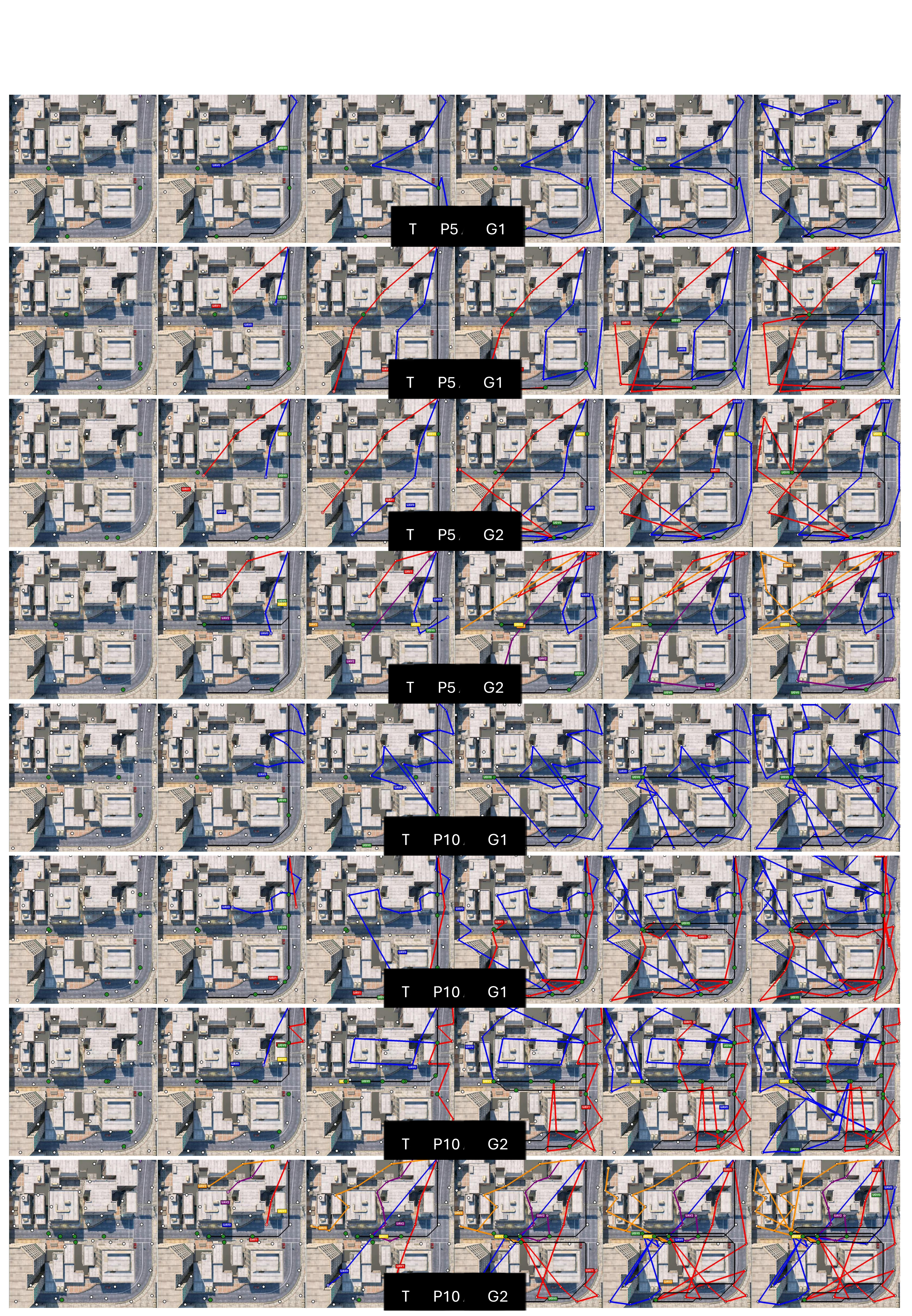
The complete city and suburban montages preserve all eight rows each. City roads differ while the initial depot matches rural; suburban moves the depot toward the map center. The displayed specialization of UAV coverage and supporting UGV routes is qualitative generalization evidence, without a separate full distribution of new-map trial success rates.
Selectable PDF text; mathematical layout is preserved above
T15-P5 A1-G1
T15-P5 A2-G1
T15-P5 A2-G2
T15-P5 A4-G2
T45-P10 A1-G1
T45-P10 A2-G1
T45-P10 A2-G2
T45-P10 A4-G2
Selectable PDF text; mathematical layout is preserved above
T15-P5 A1-G1
T15-P5 A2-G1
T15-P5 A2-G2
T15-P5 A4-G2
T45-P10 A1-G1
T45-P10 A2-G1
T45-P10 A2-G2
T45-P10 A4-G2
Appendix F.4 · Diffusion baseline variability
Supplementary Table 5 repeats the diffusion-baseline means with ± ranges described as confidence intervals. It explicitly aggregates only trials all compared methods complete. The confidence level, interval estimator, exact successful-subset counts and independent-seed structure are not specified. The prose says EMDM prioritizes high-uncertainty variables, whereas the method defines minimum-entropy selection; both original statements are retained, and the table alone cannot resolve that wording discrepancy.

Selectable PDF text; mathematical layout is preserved above
Mission
Method
1UAV–1UGV
2UAV–1UGV
2UAV–2UGV
4UAV–2UGV
Makespan
Energy
Makespan
Energy
Makespan
Energy
Makespan
Energy
T15-P5
VMDM (baseline)
7355.55±999.58
8120.37±2911.23
5478.12±1061.88
9222.99±3063.54
4050.49±887.78
8515.34±3952.92
3412.35±755.53
9420.57±2101.88
EMDM (baseline)
6917.06±877.28
6543.11±1675.89
4395.18±717.11
9744.47±2918.72
3955.99±743.15
6909.90±3192.38
3190.77±449.94
8350.71±1912.61
MEND (ours)
6650.30±653.36
5893.97±1617.99
4026.77±505.23
9079.82±2837.84
3917.65±528.61
6878.65±2303.70
2772.57±386.92
6966.35±1478.62
T45-P10
VMDM (baseline)
10184.85±1428.18
10496.56±3342.93
6356.85±967.62
14536.87±5216.91
5518.29±755.29
10206.61±2783.67
4716.66±2304.69
13771.02±6632.27
EMDM (baseline)
10157.86±1487.71
7826.26±2001.03
6093.69±940.97
10932.93±4452.93
5506.65±634.97
9773.20±2729.86
4601.49±1532.36
12435.69±4903.64
MEND (ours)
10108.99±1423.56
7502.81±2090.63
5957.50±373.81
10555.20±4148.33
5290.29±458.22
9110.07±2419.15
4555.97±1191.44
12114.19±4741.51
Original supplementary video
The unchanged original supplementary movie and poster are archived from the primary project. The video illustrates the method, simulation and mixed-reality robot coordination. The original movie retains its displayed playback accelerations, including 14× suburban, 4× city and 3× mixed-reality clips. Selected demonstrations do not add independent quantitative trials or establish electrical recharge performance beyond the manuscript’s reported setup.