Overview
Explicit-energy action refinement, a trajectory-consistency warning score, and intervention-driven retraining. All original figures, tables, displayed mathematics, algorithms and references are retained. Source code.
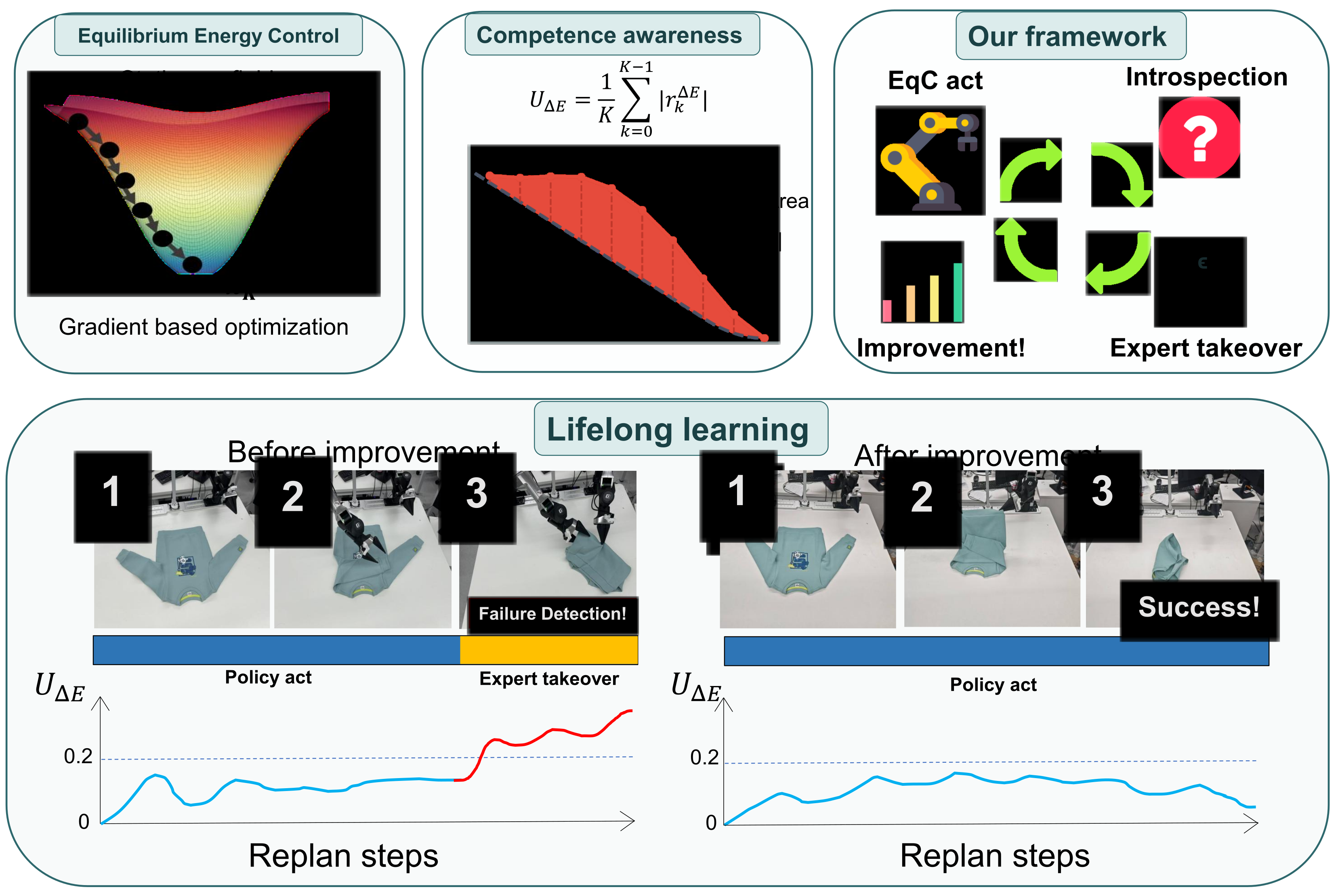
At a glance
EqC learns a scalar landscape whose action gradients refine a noisy action chunk. Comparing energy progress along that refinement path with the training bridge produces a warning signal; persistent alarms request expert recovery, and accumulated recoveries retrain the policy. Simulation and small real-robot studies report better control and failure discrimination. The theory establishes properties of the learned landscape, not action correctness or guaranteed failure detection; long-term transfer remains open.
1 Introduction
A deployed policy needs both useful actions and a way to request help when execution becomes unreliable. EqC connects these functions through one conditional energy model: optimize actions, inspect the optimization path, and collect recovery demonstrations where that path is inconsistent. Unlike a static action generator, its deployment loop includes targeted data acquisition and repeated offline updates. “Competence expansion” refers to improved autonomy on the tested tasks after those updates, not unrestricted self-improvement.
2 Related Work
The approach joins generative control, energy-based inference and robot-gated imitation learning. Its distinguishing mechanism is the finite change in explicit energy along the same path used to produce actions.
Generative models for robotics.
Diffusion and flow-matching policies refine noisy action candidates iteratively. EqC retains that computational pattern while replacing an unconstrained denoising/velocity field with the gradient of a scalar energy. It builds on architectures such as π0 and diffusion transformers rather than introducing a new perception backbone.
Energy-based models for robotics.
Earlier energy policies optimize observation–action compatibility, and Equilibrium Matching and GeCO use stationary refinement with implicit energy structure. EqC makes the deployed scalar explicit, so its change along a path can be measured. This differs from using only the terminal energy as confidence.
Failure detection and competence-aware autonomy.
DAgger aggregates on-policy expert corrections; robot-gated variants decide when to ask for them. Diff-DAgger uses denoising/flow loss as a warning signal. EqC instead compares observed energy progress with a bridge-derived reference and requires persistent violations before takeover.
3 EqC for Introspective Lifelong Robot Learning
The formulation separates learning a stationary energy gradient, reading its refinement geometry, and using that signal in a recovery-and-retraining loop.
3.1 Overview
Given observation, instruction and robot state, the energy ranks candidate action chunks. Gradient ascent generates a chunk; path consistency measures agreement with the learned bridge relation; an alarm gate determines whether to execute the prefix or request recovery.
3.2 Equilibrium Energy Control
Interpolate from Gaussian noise ε to demonstration a using xₜ=ε+t(a−ε), with t=0 at noise and t=1 at data. Train ∇ₓE to match c(t)(a−ε), normalized by active action dimension. At deployment the field receives x and condition z but no bridge time: initialize noise, take K ascent steps, execute a short prefix and replan. Smoothness and sufficiently small steps imply increasing learned energy, without guaranteeing task success.
Equations 1–2
| (1) |
| (2) |
Architecture compatibility.
The implementation forms E(x,z)=〈x,f(x,z)〉 over active action coordinates and differentiates the entire scalar, including f’s dependence on x. Training therefore requires higher-order differentiation. DiT and VLA models share this scalar interface; π0 retains its multimodal prefix/action expert and padding mask while fixing model time to zero.
3.3 Introspection from Energy Geometry
Perfect bridge-gradient matching implies E(a)−E(xₜ)=‖a−ε‖²C(t). At inference, use the predicted endpoint as a self-anchor, project iterates onto the initial-noise-to-endpoint chord, normalize energy-to-go by a floored squared chord length, and average absolute deviations from C. The signal needs no test-time expert or auxiliary uncertainty model. Main Equation 4 averages k=0,…,K−1, whereas Appendix Equation 62 uses k=1,…,K; both originals are retained, and the paper does not reconcile that indexing difference. Self-consistency alone can miss a confidently wrong trajectory.
Equations 3–4
| (3) |
| (4) | ||||
3.4 Energy-Gated DAgger for Lifelong Robot Learning
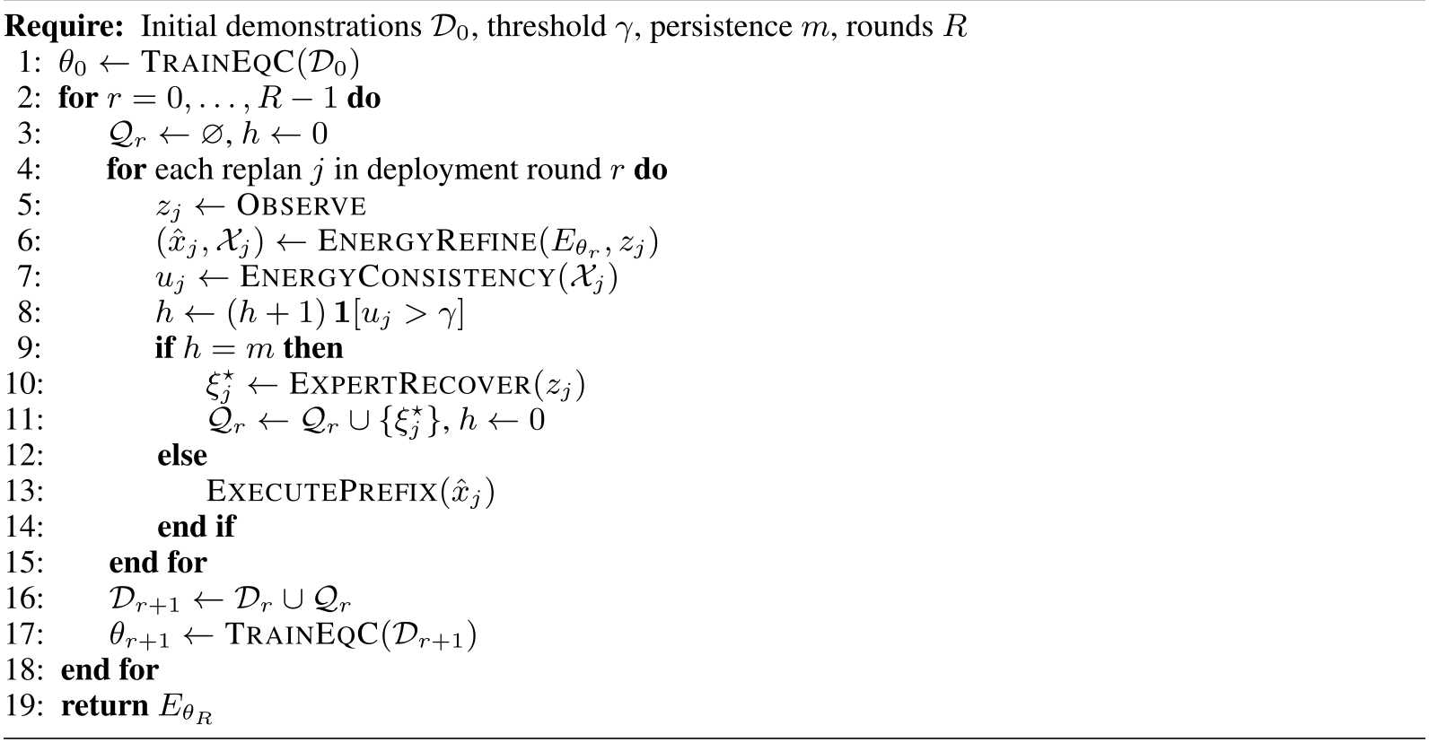
Before each action prefix, compare the score with a threshold. After m consecutive exceedances, pause autonomous execution, obtain an expert recovery and save it. Subsequent rounds train on the cumulative demonstration set. Persistence rejects isolated spikes, but thresholds, window size and expert availability remain parts of the operating protocol.
4 Why EqC Fits Generative Robot Policies
The argument for explicit energy combines a favorable conditional action-generation setting with bounds on representation and optimization. These are sufficient conditions and structural properties, not a universal superiority result.
A favorable generation regime.
Rich observations and instructions may narrow valid actions; control needs one successful action and replans after a short prefix. Smaller outputs and concentrated conditional targets may therefore make stationary optimization practical. This motivation does not establish that all robotics tasks have low action ambiguity or recoverable bridge progress.
Approximation and optimization.
A radial witness bounds the excess risk of stationary energy gradients relative to a time-conditioned regressor by action dispersion, uncertainty in recovering bridge scale, and neural approximation error. Separate results give monotone ascent under local smoothness and stable steps, and decompose the warning residual into chord-wise field mismatch, off-chord motion and normalization effects. None proves that a low residual means a safe or correct action.
Equation 5
| (5) |
5 Experiments
Evaluation covers action generation, rollout-level failure detection, and repeated recovery-data collection. Published benchmark baselines, independent reproductions, calibrated operating metrics and qualitative examples are distinguished below.
5.1 Simulated and Real-World Benchmarks
Control comparisons use common task-success definitions within each benchmark. The real-robot results cover three manipulation tasks on one bimanual platform.
5.1.1 Setup
DiT comparisons share architecture, demonstrations and action interface; VLA comparisons retain the underlying multimodal backbone within each pair. Benchmarks include LIBERO, five RoboTwin tasks, five standardized VLABench tracks and seven LIBERO-Plus perturbation families. These controlled comparisons do not make data budgets identical across unrelated published methods.
5.1.2 Diffusion Transformer
EqC averages 93.95±0.66% across four DiT training seeds on LIBERO, rounded to 94.0% in the main table. The main table mixes this mean with published baseline values. Independent matched reproductions in Appendix A give rectified flow 89.12±0.80% and GeCO 92.30±1.02%; these are the more direct multi-seed comparison.
5.1.3 Vision-Language-Action Policies
The VLA variant evaluates the π0 action expert at model time zero, scalarizes its features with the action, and trains the resulting gradient. Active-coordinate masking prevents padded embodiment dimensions from entering the energy objective. Improvements are measured after benchmark-specific fine-tuning, except the direct LIBERO-to-LIBERO-Plus transfer.
(a) RoboTwin 2.0 (Easy / Hard)
| Method | Bottle | Hammer | Rank | Alarm | Bell | Avg. |
|---|---|---|---|---|---|---|
| 90 / 56 | 43 / 21 | 7 / 1 | 63 / 11 | 44 / 3 | 49 / 18 | |
| + GeCO | 88 / 66 | 52 / 36 | 0 / 0 | 72 / 16 | 42 / 21 | 50 / 28 |
| + EqC (ours) | 100 / 76 | 76 / 27 | 6 / 0 | 83 / 32 | 49 / 30 | 63 / 33 |
RoboTwin 2.0.
Across five RoboTwin tasks and 100 episodes per task/setting, π0 improves from 49% Easy / 18% Hard to 63% / 33% with EqC, versus 50% / 28% with GeCO. Gains vary by task; the experiment covers this selected subset rather than the entire benchmark.
VLABench.
VLABench averages increase from 29.4% to 36.7% for π0 and from 24.5% to 27.1% for π0.5 across T1–T4 and T6. T5 is excluded because the official cross-task setting has no fixed standardized split. The two backbone configurations also use different training batch sizes.
LIBERO-Plus.
Direct evaluation of the LIBERO-trained policy on LIBERO-Plus raises the aggregate from 53.6% to 65.8%. Camera-shift success rises from 15.8% to 61.7%, and robot-initialization success from 6.6% to 39.0%. Improvements are not uniform across every perturbation; language and sensor-noise success, for example, are lower in the displayed table.
5.1.4 Real-World Experiments
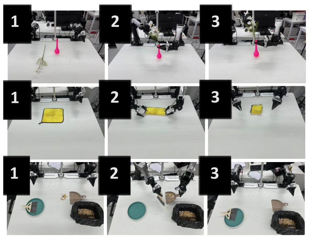
With 20 trials per task on two Galaxea A1Z arms, EqC improves flower insertion from 45% to 80%, towel folding from 80% to 95%, and sweeping from 65% to 100%, giving 63.3%→91.7% average success. Average inference latency increases from 432.4 to 543.9 ms (about 26%). These are finite task-level success counts, without a reported multi-seed physical control comparison.
(a) Real-world bimanual manipulation
| Success (%) | Latency (ms) | |||||||
|---|---|---|---|---|---|---|---|---|
| Method | Flower | Towel | Sweep. | Avg. | Flower | Towel | Sweep. | Avg. |
| Galaxea G0.5 | 45.0 | 80.0 | 65.0 | 63.3 | 421.9 | 435.6 | 439.6 | 432.4 |
| Galaxea G0.5 + EqC (ours) | 80.0 | 95.0 | 100.0 | 91.7 | 526.4 | 556.5 | 548.7 | 543.9 |
5.2 Competence Awareness
Competence awareness is evaluated against final rollout success/failure, so an unusual but successful scene is a negative example. The warning score is an empirical failure predictor, not an observation-novelty classifier.
5.2.1 Setup
A rollout alarms when its score stays above threshold for m replans. Failed rollouts are positives, successful ones negatives. Detection timing uses the fraction of the capped horizon remaining at the alarm; this estimates avoided remaining inference, not measured recovery time or prevented damage.
5.2.2 Simulated Rollout Analysis
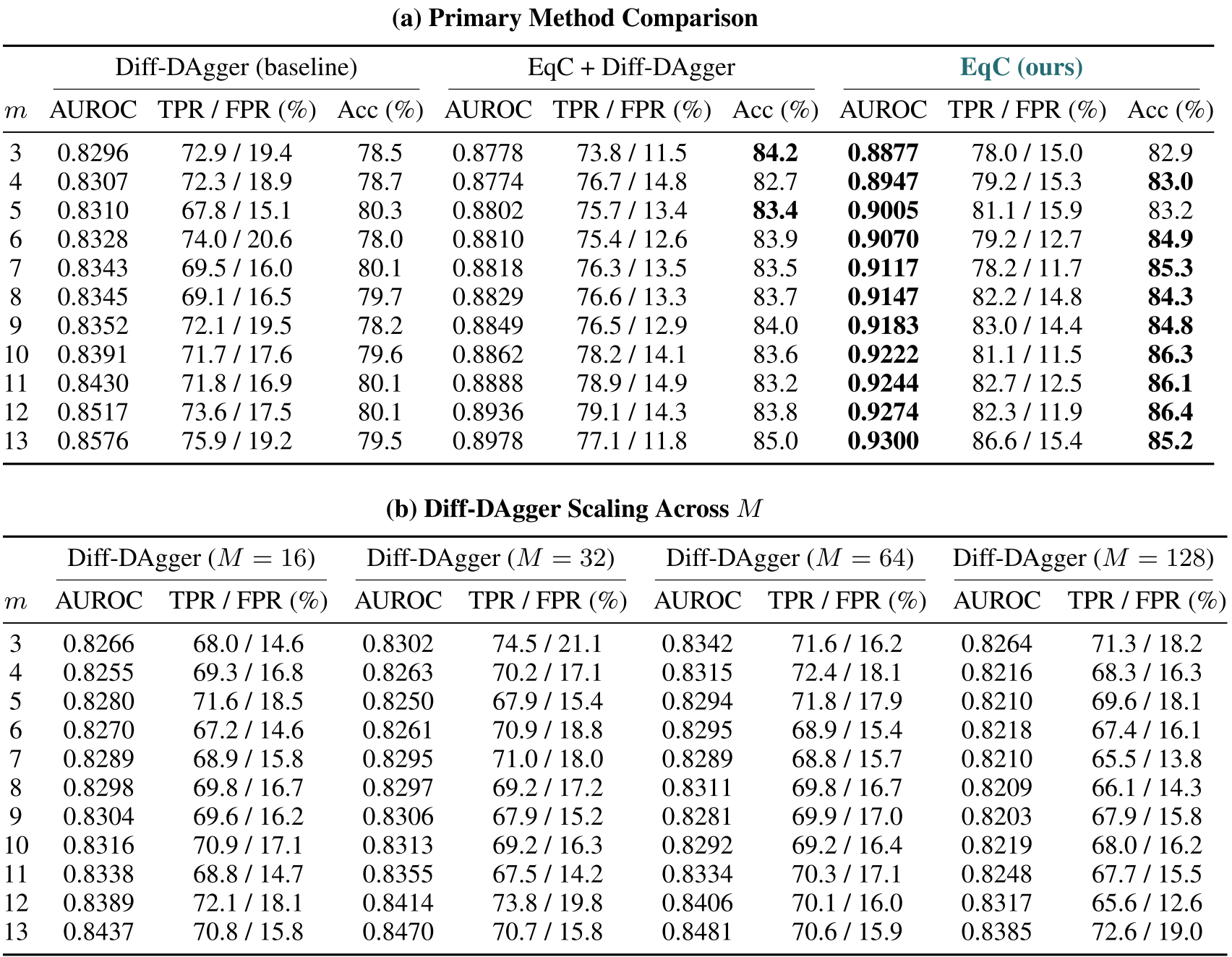
At the main operating point, EqC reports AUROC 0.9244 versus 0.8430 for Diff-DAgger and 0.8888 for the hybrid. TPR/FPR are 77.9%/8.5%, versus 61.3%/10.2% and 72.8%/8.8%; accuracy is 87.5% and remaining-horizon saving 45.5%. Thresholds/windows use 10% calibration and 90% test data. Appendix B clarifies that AUROC is descriptive over all labeled rollouts, whereas threshold-dependent metrics use the held-out test split.
5.2.3 Real-World Rollout Analysis
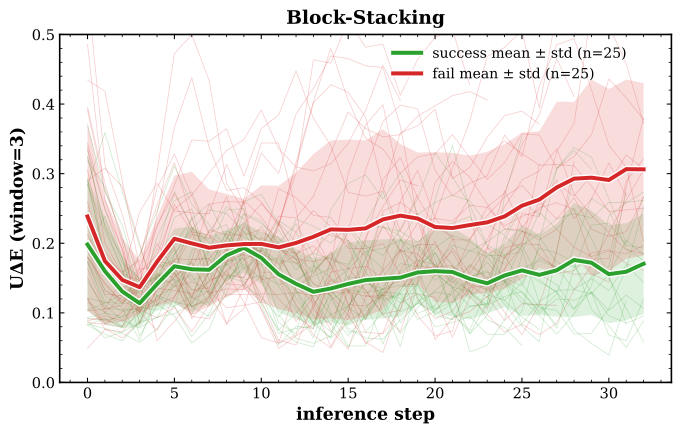
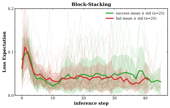
A Round-3 block-stacking checkpoint yields 25 successful and 25 failed real rollouts under nominal configurations. Three-step-smoothed EqC curves separate outcomes earlier than Diff-DAgger in Figure 3. This deliberately balanced, small analysis supports qualitative discrimination; it does not estimate natural failure prevalence or a deployment-wide false-alarm guarantee.
5.3 Energy-Gated DAgger for Lifelong Learning
The physical learning study compares intervention triggers under matched seed data, six recovery demonstrations per round and repeated training. Expert recovery remains an external source of task competence.
5.3.1 Experimental Setup and Protocol
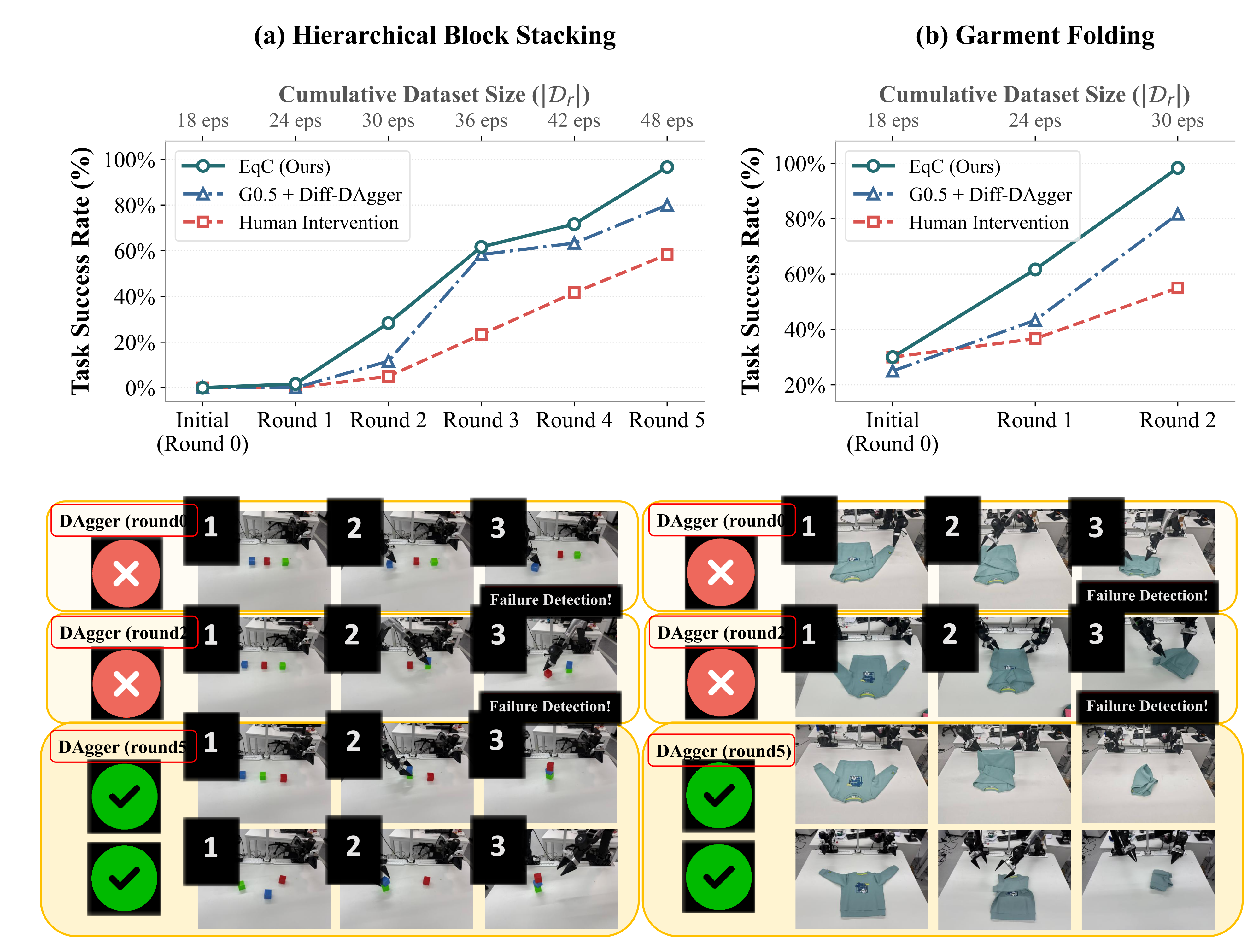
Block stacking and garment folding start with 18 demonstrations each. A fixed γ=0.2 plus persistence triggers recovery; stacking runs five collection rounds and garment folding two. After each round the cumulative data retrain the policy, and 20 fully autonomous trials measure the resulting checkpoint.
5.3.2 Progressive Performance
The PDF Figure 4 and Table 17 are used here: the HTML plot asset contains inconsistent lower curves, so the PDF composite is restored. Across three complete runs, stacking reaches 96.7±2.9% after 30 recoveries, versus 80.0% for G0.5+Diff-DAgger and 58.3% for human-triggered intervention. Garment folding reaches 98.3±2.9% after 12 recoveries, versus 81.7% and 55.0%. The matching budgets support the tested trigger comparison; they do not establish universal superiority to skilled human supervision. Separate single-run studies examine cross-task recovery and a prepared robot-agent expert.
6 Limitations and Scope
Scope is continuous action chunks with stationary refinement. Hybrid, memory-based and hierarchical policies, calibration transfer, repeated aggregation over long deployments and new embodiments remain untested. Wrong but internally coherent paths can evade the score; expert recovery and repeated offline training are still required.
7 Conclusion
EqC connects action generation and help requests through explicit energy geometry. The reported control and intervention gains support this design on the evaluated manipulation settings. Proposed extensions to locomotion, navigation and driving are future applications, not experiments in this paper.
AI use statement
The authors disclose generative-AI assistance with manuscript wording, scientific figures and code, and state that they reviewed the resulting material and take responsibility for it.
Reproducibility statement
The appendices retain mathematical derivations, model settings, calibration protocols, physical-task definitions and baseline details. Code is linked in Appendix I; the note does not independently reproduce training or robot experiments.
Appendix A Evaluation Details
The implementation appendix specifies benchmark coverage, rollout budgets, shared action interfaces and the distinction between published and independently reproduced baselines.
| Benchmark | Coverage | Episodes |
|---|---|---|
| LIBERO–DiT | 4 suites; 40 tasks | 50/task |
| LIBERO–VLA | 4 suites; 40 tasks | 50/task |
| RoboTwin 2.0 | 5 tasks; Easy and Hard | 100/task/setting |
| VLABench | Tracks 1, 2, 3, 4, and 6; 50 tasks | 50/task |
| LIBERO-Plus | 7 perturbation families | 10030 total |
A.1 Implementation Protocol
Use noise-to-data time, fix model time at zero and sum energy independently per sample over active dimensions. Training keeps the higher-order graph; inference detaches actions between ascent steps. The reported schedule is c(t)=min{4,20(1−t)}, with its remaining integral evaluated analytically; other schedules require the theory’s stated conditions.
A.2 Benchmarks
Table 4 gives exact coverage and episode budgets. Success criteria come from the benchmark or, for real tasks, the explicit completion rules in Appendix D.
LIBERO.
LIBERO has four suites of ten tasks: Goal, Spatial, Object and Long. DiT and VLA evaluations use 50 episodes per task. The suites vary goal semantics, spatial relations, object categories and multi-stage composition.
RoboTwin 2.0.
RoboTwin covers Adjust Bottle, Beat Block Hammer, Blocks Ranking by Size, Click Alarmclock and Click Bell. Each task has a dedicated fine-tuned policy and 100 evaluation episodes in each Easy/Hard setting; Hard adds domain randomization.
VLABench.
VLABench uses 50 episodes per task over 50 tasks across T1–T4 and T6: task learning, object/category generalization, commonsense, instruction semantics and appearance shifts. The open T5 cross-task track is omitted instead of defining a new private split.
LIBERO-Plus.
LIBERO-Plus tests camera, robot initialization, language, illumination, background, sensor noise and object-layout changes while preserving task semantics. The evaluation budget totals 10,030 episodes, using the LIBERO-trained checkpoint without adaptation.
A.3 DiT Details
DiT encodes vision with DINOv2-base and instructions with T5-base, observes one time step, predicts 16 actions of seven dimensions and executes the first eight. The optimized chunk therefore has 112 active coordinates.
Training.
DiT trains 70,000 steps with batch 256, mixed bf16, AdamW, 5,000 warmup steps, peak learning rate 10⁻⁴ and weight decay 10⁻⁴. These settings define the matched objective comparisons.
A.4 Multi-Seed DiT Results
Four EqC seeds yield suite means 95.60, 96.35, 98.10 and 85.50%, and overall 93.95±0.66%. Long remains the weakest suite. Table 6’s independent rectified-flow and GeCO reproductions are separate from the published baselines in the main table; the latter are not presented as newly rerun.
A.5 VLA Training Details
OpenPI π0/π0.5 checkpoints are fine-tuned with AdamW, gradient norm clipping at 1, cosine decay, 10,000 warmup steps and peak learning rate 5×10⁻⁵. Training lasts 50,000 steps for LIBERO and 30,000 for RoboTwin/VLABench.
RoboTwin 2.0.
Each RoboTwin task uses batch 32, three RGB cameras and proprioception. The action chunk spans 50 steps and 14 active coordinates per step, totaling 700 optimized dimensions.
LIBERO and LIBERO-Plus.
LIBERO π0 uses the physical-intelligence/libero dataset, batch 32 and 50,000 steps. Its checkpoint transfers directly to all seven LIBERO-Plus perturbation suites, with no benchmark-specific fine-tuning.
VLABench.
VLABench uses the released primitive fine-tuning dataset for 30,000 steps. Batch sizes are 256 for π0 and 32 for π0.5, so their absolute results are not a batch-matched comparison between backbones.
A.6 Supplementary LIBERO Results for VLA Policies
The supplementary VLA LIBERO result averages 94.3%, versus π0 at 94.2% and π0+GeCO at 93.9%. EqC gains on Long but has lower Goal success than GeCO. The small aggregate advantage here complements, rather than matches the size of, gains on robustness benchmarks.
| Method | Goal | Spatial | Object | Long | Avg. |
|---|---|---|---|---|---|
| + FAST (Pertsch et al., 2025) | 88.6 | 96.4 | 96.8 | 60.2 | 85.5 |
| 95.8 | 96.8 | 98.8 | 85.2 | 94.2 | |
| + GeCO | 96.4 | 96.8 | 97.0 | 85.4 | 93.9 |
| + EqC (ours) | 94.6 | 97.6 | 98.8 | 86.2 | 94.3 |
Appendix B Competence Awareness Details
The detector appendix defines rollout-level labels, calibration, baseline scoring, alternative operating points and computation costs. It separates held-out operational estimates from full-data descriptive/oracle analyses.
B.1 Task Definition: Online Failure Detection
Labels reflect final task outcome: unfamiliar success is negative and nominal failure positive. This makes the detector relevant to intervention decisions, but retrospective success labels do not by themselves identify the precise last recoverable instant.
B.2 Simulation Failure Detection Protocol
Whole rollouts are assigned to disjoint 10% calibration and 90% test splits, stratified by original LIBERO plus seven perturbation families. Checkpoints are fixed before calibration. Choose persistence and threshold by approximately 10% calibration FPR or by Youden’s J; freeze them for test metrics. AUROC is separately swept over all labeled rollouts. The comparison shares initial-instance split membership, while policies can generate different trajectories and outcomes. Time saved is 100(1−alarm step/capped horizon), an inference-horizon proxy.
B.3 Real-World Failure Detection Protocol
Real-world detection uses the intermediate stacking checkpoint trained on 36 cumulative demonstrations. Fifty nominal-layout rollouts are selected as 25 successes and 25 failures. A three-step moving average precedes the persistence gate; this differs from treating each raw replanning sample as an independent test example.
B.4 Composition of the Calibration Split
The 1,203-rollout calibration set is stratified across eight dataset variants, with 200 original-LIBERO cases and 108–160 per perturbation family. Suite shares happen to be roughly 25% after random within-family sampling; suites are not separately stratified. Different policies may have different outcome labels for corresponding instances.
| Dataset | Count | Ratio (%) |
|---|---|---|
| Original LIBERO | 200 | 16.63 |
| Camera | 160 | 13.30 |
| Noise | 160 | 13.30 |
| Robot | 155 | 12.88 |
| Language | 154 | 12.80 |
| Layout | 152 | 12.64 |
| Light | 114 | 9.48 |
| Background | 108 | 8.98 |
B.5 Diff-DAgger Baseline Implementation Adapted for π 0
Diff-DAgger first generates an action chunk, treats it as a pseudo-label, then samples fresh noise and Beta(1.5,1) bridge times to measure normalized flow error. It masks padded dimensions and averages M Monte Carlo evaluations; default M=10, versus K=10 EqC refinements in this simulation comparison. These are re-noising/time samples, although later prose calls them dropout samples. The π0 bridge convention in this baseline is reversed relative to EqC’s noise-to-data notation.
Equations 6–12
| (6) |
| (7) |
| (8) |
| (9) |
| (10) |
| (11) |
| (12) |
B.6 Detailed Results
Across m=3–13, EqC’s all-rollout AUROC rises from 0.8877 to 0.9300, ahead of the compared signals. Calibrated FPR is not an exact test guarantee: held-out values vary. Larger persistence generally trades timing for discrimination, and EqC does not win every time-saving cell. Tables 11–12 optimize thresholds on the full evaluation set; their “theoretical upper bound” is an empirical oracle analysis, not a mathematical bound or held-out operating result. Increasing Diff-DAgger samples does not close the observed gap. Per-replan JAX latency is 108.86 ms for EqC, 79.44 ms for M=10 Diff-DAgger and 171.03 ms for the hybrid; EqC is not universally fastest.
| Diff-DAgger | EqC + Diff-DAgger | EqC (ours) | |||||||
|---|---|---|---|---|---|---|---|---|---|
| AUROC | TPR / FPR (%) | Acc (%) | AUROC | TPR / FPR (%) | Acc (%) | AUROC | TPR / FPR (%) | Acc (%) | |
| 3 | 0.8296 | 58.1 / 9.1 | 82.1 | 0.8778 | 71.9 / 9.9 | 84.8 | 0.8877 | 69.5 / 9.1 | 84.6 |
| 4 | 0.8307 | 56.3 / 8.3 | 82.2 | 0.8774 | 70.4 / 8.8 | 85.1 | 0.8947 | 70.8 / 8.9 | 85.1 |
| 5 | 0.8310 | 57.1 / 8.6 | 82.2 | 0.8802 | 70.9 / 9.3 | 84.9 | 0.9005 | 70.7 / 7.9 | 85.8 |
| 6 | 0.8328 | 55.7 / 8.1 | 82.2 | 0.8810 | 71.2 / 9.2 | 85.1 | 0.9070 | 74.7 / 9.0 | 86.2 |
| 7 | 0.8343 | 58.3 / 9.2 | 82.1 | 0.8818 | 71.7 / 8.9 | 85.4 | 0.9117 | 74.8 / 9.1 | 86.1 |
| 8 | 0.8345 | 59.8 / 9.9 | 82.0 | 0.8829 | 72.4 / 9.5 | 85.2 | 0.9147 | 76.1 / 9.3 | 86.3 |
| 9 | 0.8352 | 61.5 / 11.0 | 81.6 | 0.8849 | 73.5 / 9.8 | 85.3 | 0.9183 | 76.7 / 8.9 | 86.9 |
| 10 | 0.8391 | 60.3 / 10.1 | 82.0 | 0.8862 | 72.5 / 9.1 | 85.5 | 0.9222 | 77.7 / 8.9 | 87.1 |
| 11 | 0.8430 | 61.3 / 10.2 | 82.2 | 0.8888 | 72.8 / 8.8 | 85.8 | 0.9244 | 77.9 / 8.5 | 87.5 |
| 12 | 0.8517 | 62.3 / 9.2 | 83.2 | 0.8936 | 74.6 / 10.4 | 85.2 | 0.9274 | 78.4 / 8.4 | 87.6 |
| 13 | 0.8576 | 63.8 / 9.9 | 83.1 | 0.8978 | 74.0 / 9.2 | 85.9 | 0.9300 | 78.9 / 9.0 | 87.4 |
| Diff-DAgger | EqC + Diff-DAgger | EqC (ours) | |||||||
|---|---|---|---|---|---|---|---|---|---|
| AUROC | TPR / FPR (%) | Acc (%) | AUROC | TPR / FPR (%) | Acc (%) | AUROC | TPR / FPR (%) | Acc (%) | |
| 3 | 0.8296 | 73.9 / 20.8 | 77.8 | 0.8778 | 78.3 / 16.9 | 81.7 | 0.8877 | 78.1 / 14.9 | 83.0 |
| 4 | 0.8307 | 65.2 / 13.3 | 80.9 | 0.8774 | 80.6 / 19.5 | 80.5 | 0.8947 | 82.4 / 20.0 | 80.7 |
| 5 | 0.8310 | 76.0 / 24.4 | 75.7 | 0.8802 | 79.2 / 16.8 | 82.0 | 0.9005 | 82.1 / 17.5 | 82.4 |
| 6 | 0.8328 | 73.0 / 19.9 | 78.2 | 0.8810 | 80.0 / 18.1 | 81.4 | 0.9070 | 79.4 / 13.0 | 84.7 |
| 7 | 0.8343 | 75.0 / 23.2 | 76.3 | 0.8818 | 78.6 / 15.9 | 82.5 | 0.9117 | 85.3 / 20.2 | 81.4 |
| 8 | 0.8345 | 70.4 / 18.9 | 78.2 | 0.8829 | 76.9 / 13.7 | 83.6 | 0.9147 | 81.9 / 14.5 | 84.4 |
| 9 | 0.8352 | 65.5 / 14.5 | 80.2 | 0.8849 | 73.8 / 10.1 | 85.2 | 0.9183 | 83.8 / 15.5 | 84.3 |
| 10 | 0.8391 | 71.3 / 17.6 | 79.4 | 0.8862 | 80.8 / 18.0 | 81.7 | 0.9222 | 84.0 / 14.7 | 85.0 |
| 11 | 0.8430 | 70.3 / 16.4 | 80.1 | 0.8888 | 78.1 / 14.2 | 83.6 | 0.9244 | 82.1 / 11.8 | 86.4 |
| 12 | 0.8517 | 65.1 / 11.0 | 82.6 | 0.8936 | 77.5 / 12.7 | 84.4 | 0.9274 | 87.5 / 18.3 | 83.4 |
| 13 | 0.8576 | 69.0 / 13.6 | 81.7 | 0.8978 | 74.6 / 9.6 | 85.8 | 0.9300 | 85.5 / 14.5 | 85.5 |
| FPR-Constrained Calibration | Youden’s Index Calibration | |||||
| Diff-DAgger | EqC + Diff | EqC (ours) | Diff-DAgger | EqC + Diff | EqC (ours) | |
| 3 | 33.6 | 44.5 | 45.2 | 47.9 | 51.8 | 53.7 |
| 4 | 31.8 | 42.5 | 45.3 | 39.2 | 53.8 | 57.4 |
| 5 | 32.1 | 42.7 | 44.5 | 49.4 | 51.8 | 55.5 |
| 6 | 30.6 | 42.6 | 46.7 | 45.2 | 52.2 | 51.5 |
| 7 | 32.0 | 42.8 | 46.6 | 47.0 | 50.2 | 57.1 |
| 8 | 32.5 | 43.0 | 46.3 | 42.4 | 47.9 | 52.2 |
| 9 | 33.9 | 43.5 | 46.2 | 37.4 | 43.8 | 53.7 |
| 10 | 32.7 | 42.4 | 46.0 | 41.8 | 51.0 | 53.0 |
| 11 | 33.3 | 42.1 | 45.5 | 40.4 | 47.9 | 49.8 |
| 12 | 33.3 | 43.8 | 45.3 | 35.4 | 46.4 | 54.8 |
| 13 | 34.3 | 42.4 | 45.3 | 38.6 | 42.9 | 51.5 |
| Method | Orig. | Camera | Robot | Lang. | Light | Backgr. | Noise | Layout | W. Avg. |
|---|---|---|---|---|---|---|---|---|---|
| Diff-DAgger () | 27.7 | 50.5 | 50.1 | 46.4 | 30.0 | 34.0 | 44.1 | 47.9 | 46.1 |
| Diff-DAgger () | 26.5 | 44.2 | 46.0 | 39.9 | 32.5 | 32.3 | 37.3 | 44.9 | 41.5 |
| Diff-DAgger () | 28.9 | 47.2 | 48.6 | 44.1 | 33.8 | 34.5 | 43.1 | 46.1 | 44.6 |
| Diff-DAgger () | 27.0 | 45.0 | 47.5 | 44.1 | 33.8 | 28.0 | 39.0 | 44.0 | 42.7 |
| Diff-DAgger () | 23.5 | 41.3 | 42.4 | 37.4 | 28.5 | 30.2 | 35.1 | 40.6 | 38.4 |
| Diff-DAgger () | 25.9 | 42.8 | 43.5 | 39.0 | 30.7 | 30.5 | 37.1 | 41.8 | 39.8 |
| Diff-DAgger () | 28.1 | 48.5 | 48.3 | 42.8 | 34.9 | 34.4 | 38.5 | 45.6 | 43.9 |
| Diff-DAgger () | 28.3 | 40.4 | 42.9 | 34.8 | 31.1 | 28.7 | 36.1 | 38.9 | 38.0 |
| Diff-DAgger () | 28.6 | 42.9 | 44.1 | 37.4 | 32.3 | 31.3 | 38.6 | 40.6 | 40.0 |
| EqC + Diff-DAgger () | 30.7 | 50.3 | 51.8 | 56.9 | 44.1 | 27.0 | 44.5 | 48.9 | 49.1 |
| EqC + Diff-DAgger () | 30.3 | 51.4 | 50.8 | 53.7 | 42.6 | 29.1 | 46.3 | 48.3 | 48.5 |
| EqC + Diff-DAgger () | 26.8 | 48.4 | 47.0 | 50.2 | 40.8 | 26.4 | 43.5 | 45.2 | 45.3 |
| EqC (ours)() | 26.7 | 54.8 | 57.3 | 70.7 | 41.7 | 29.0 | 40.1 | 55.4 | 54.0 |
| EqC (ours)() | 24.7 | 53.4 | 55.3 | 60.8 | 39.7 | 30.2 | 41.5 | 47.8 | 50.5 |
| EqC (ours)() | 26.7 | 56.4 | 58.2 | 61.0 | 40.3 | 32.2 | 46.1 | 49.5 | 52.8 |
| Method | Mean Latency (ms) |
|---|---|
| Diff-DAgger () | 79.44 |
| Diff-DAgger () | 91.43 |
| Diff-DAgger () | 122.11 |
| EqC + Diff-DAgger () | 171.03 |
| EqC (ours) | 108.86 |
B.7 Extended Studies
Terminal energy gives weak discrimination (AUROC about 0.52–0.65); final gradient norm improves it to about 0.87, while full-path consistency reaches 0.93. Energy differences cancel arbitrary additive condition offsets that can affect absolute energy. These ablations support using trajectory geometry, without establishing complete detection of all failure mechanisms.
| Terminal Energy | Last-step Gradient Norm | EqC (ours) | |||||||
|---|---|---|---|---|---|---|---|---|---|
| AUROC | TPR / FPR (%) | Acc (%) | AUROC | TPR / FPR (%) | Acc (%) | AUROC | TPR / FPR (%) | Acc (%) | |
| 3 | 0.5237 | 17.1 / 10.0 | 68.4 | 0.8734 | 68.0 / 9.3 | 84.0 | 0.8877 | 69.5 / 9.1 | 84.6 |
| 4 | 0.5404 | 19.3 / 10.1 | 68.9 | 0.8707 | 67.1 / 9.1 | 83.9 | 0.8947 | 70.8 / 8.9 | 85.1 |
| 5 | 0.5604 | 23.1 / 10.3 | 69.9 | 0.8713 | 65.5 / 8.7 | 83.6 | 0.9005 | 70.7 / 7.9 | 85.8 |
| 6 | 0.5754 | 26.0 / 10.8 | 70.5 | 0.8724 | 65.7 / 9.4 | 83.2 | 0.9070 | 74.7 / 9.0 | 86.2 |
| 7 | 0.5861 | 26.8 / 10.2 | 71.1 | 0.8737 | 66.0 / 9.3 | 83.3 | 0.9117 | 74.8 / 9.1 | 86.1 |
| 8 | 0.5974 | 28.7 / 9.8 | 71.9 | 0.8737 | 66.2 / 9.5 | 83.3 | 0.9147 | 76.1 / 9.3 | 86.3 |
| 9 | 0.6082 | 29.9 / 9.4 | 72.6 | 0.8744 | 64.7 / 9.0 | 83.2 | 0.9183 | 76.7 / 8.9 | 86.9 |
| 10 | 0.6214 | 32.5 / 10.0 | 72.9 | 0.8758 | 64.2 / 8.5 | 83.4 | 0.9222 | 77.7 / 8.9 | 87.1 |
| 11 | 0.6309 | 33.1 / 9.6 | 73.4 | 0.8769 | 65.4 / 9.3 | 83.1 | 0.9244 | 77.9 / 8.5 | 87.5 |
| 12 | 0.6410 | 33.8 / 9.6 | 73.6 | 0.8766 | 64.1 / 8.8 | 83.1 | 0.9274 | 78.4 / 8.4 | 87.6 |
| 13 | 0.6489 | 34.9 / 9.7 | 73.8 | 0.8766 | 64.6 / 8.8 | 83.3 | 0.9300 | 78.9 / 9.0 | 87.4 |
| Terminal Energy | Last-step Gradient Norm | EqC (ours) | |||||||
|---|---|---|---|---|---|---|---|---|---|
| AUROC | TPR / FPR (%) | Acc (%) | AUROC | TPR / FPR (%) | Acc (%) | AUROC | TPR / FPR (%) | Acc (%) | |
| 3 | 0.5237 | 21.6 / 13.2 | 67.5 | 0.8734 | 67.6 / 9.0 | 84.0 | 0.8877 | 78.1 / 14.9 | 83.0 |
| 4 | 0.5404 | 22.5 / 12.4 | 68.3 | 0.8707 | 67.7 / 9.5 | 83.8 | 0.8947 | 82.4 / 20.0 | 80.7 |
| 5 | 0.5604 | 42.5 / 32.8 | 59.9 | 0.8713 | 64.3 / 7.8 | 83.9 | 0.9005 | 82.1 / 17.5 | 82.4 |
| 6 | 0.5754 | 24.0 / 9.0 | 71.1 | 0.8724 | 72.1 / 14.1 | 81.8 | 0.9070 | 79.4 / 13.0 | 84.7 |
| 7 | 0.5861 | 28.3 / 11.5 | 70.6 | 0.8737 | 68.6 / 11.0 | 83.0 | 0.9117 | 85.3 / 20.2 | 81.4 |
| 8 | 0.5974 | 34.5 / 17.4 | 68.4 | 0.8737 | 65.3 / 9.1 | 83.3 | 0.9147 | 81.9 / 14.5 | 84.4 |
| 9 | 0.6082 | 36.7 / 16.1 | 69.9 | 0.8744 | 76.0 / 16.4 | 81.4 | 0.9183 | 83.8 / 15.5 | 84.3 |
| 10 | 0.6214 | 33.6 / 11.0 | 72.5 | 0.8758 | 75.8 / 16.3 | 81.4 | 0.9222 | 84.0 / 14.7 | 85.0 |
| 11 | 0.6309 | 48.1 / 25.6 | 66.6 | 0.8769 | 72.5 / 13.4 | 82.4 | 0.9244 | 82.1 / 11.8 | 86.4 |
| 12 | 0.6410 | 49.7 / 24.0 | 68.2 | 0.8766 | 80.7 / 21.6 | 79.1 | 0.9274 | 87.5 / 18.3 | 83.4 |
| 13 | 0.6489 | 44.4 / 18.1 | 70.8 | 0.8766 | 80.4 / 20.9 | 79.5 | 0.9300 | 85.5 / 14.5 | 85.5 |
Appendix C Theory: Assumptions and Guarantees
The theory develops a bridge identity, a stationary radial approximation witness, monotone ascent and a decomposition of the self-consistency score. Every displayed derivation is retained; the edited explanation emphasizes assumptions and what each result actually establishes.
C.1 Problem Setup
Draw expert action/condition and independent Gaussian noise; interpolate on a straight bridge and target c(t)(a−ε), with continuous nonnegative c and c(1)=0. A stationary scalar energy supplies the field through its action gradient. The finite energy target is the integral of that field along the bridge; deployed ascent starts from fresh noise.
Equations 13–17
| (13) |
| (14) |
| (15) |
| (16) |
| (17) |
C.2 From Local Gradient Matching to Path Consistency
The fundamental theorem of calculus makes energy inconsistency exactly the integral of local gradient error projected onto the demonstration displacement. Cauchy–Schwarz then bounds it by displacement length, remaining bridge length and accumulated squared field error. Small training field error therefore controls this bridge relation, but a small integral can still hide cancelling local errors.
Equations 18–21
| (18) |
| (19) |
| (20) |
| (21) |
C.3 Stationary Representation of the Bridge Target
Write the bridge coefficient as α(T)=c(T)/(1−T), and compare actions with their condition-dependent mean. A radial scale λ(radius,z) approximates α without receiving time. Conditional expectation minimizes its weighted squared error; integrating −rλ(r) constructs a conservative witness. Orthogonality, Jensen and Minkowski yield excess risk bounded by the squared sum of action dispersion, scale-recovery error and energy-class approximation error. Exact representation requires concentrated conditional actions, zero residual scale uncertainty and a class containing the witness. This sufficient single-basin construction neither diagnoses those conditions empirically nor excludes multimodal energies.
Equations 22–48
| (22) |
| (23) |
| (24) |
| (25) |
| (26) | ||||
| (27) |
| (28) |
| (29) |
| (30) |
| (31) |
| (32) |
| (33) |
| (34) |
| (35) |
| (36) |
| (37) |
| (38) |
| (39) |
| (40) |
| (41) |
| (42) |
| (43) | ||||||
| (44) |
| (45) |
| (46) |
| (47) |
| (48) |
C.4 Monotone Energy Ascent
If the gradient is locally L-Lipschitz along each update segment and 0<η<2/L, exact ascent increases E by at least η(1−Lη/2)‖∇E‖². Summing gives a bound on the smallest observed gradient norm; a bounded-above energy supplies a finite-step stationarity estimate. The guarantee concerns the learned scalar and assumed step sizes, not global optimization, task reward, or physical stability.
Equations 49–55
| (49) |
| (50) |
| (51) |
| (52) |
| (53) |
| (54) |
| (55) |
C.5 Energy Consistency as a Path-Wise Mismatch Certificate
Project each iterate onto the initial-to-final chord. The residual decomposes into integrated longitudinal field mismatch, an energy difference from off-chord motion, and a correction from flooring the squared chord norm. A bound on off-chord gradients sandwiches the observed score around mean integrated mismatch with explicit correction terms. When the floor is inactive and all iterates lie on the chord, equality gives the clean mismatch interpretation. Absolute averaging prevents cancellation between iterates, but not within each remaining-work integral; endpoint self-anchoring can still validate an incorrect path.
Equations 56–73
| (56) |
| (57) |
| (58) |
| (59) |
| (60) |
| (61) |
| (62) |
| (63) |
| (64) |
| (65) |
| (66) |
| (67) |
| (68) |
| (69) |
| (70) |
| (71) |
| (72) |
| (73) |
C.6 Scope of the auxiliary analysis
The paper explicitly limits the claims: conditional concentration is motivated, not measured or proved; the radial witness supplies an existence upper bound; energy ascent is not action correctness; and coherent wrong trajectories can have small scores. Short chords activate the normalization correction. These limits prevent interpreting the score as a calibrated probability or safety certificate.
Appendix D Real-Robot Experimental Setup and Evaluation Protocol
Physical evaluation uses one bimanual Galaxea setup, explicit completion criteria and matched collection schedules for intervention comparisons. Task definitions and budgets are retained in full original tables.
D.1 Platform and Hardware Architecture
Two six-axis A1Z arms with parallel grippers provide 14 active control channels. Three synchronized RGB cameras and 14-dimensional proprioception condition G0.5. Control runs at 15 Hz with 32-step action chunks. The platform-specific demonstration and inference settings constrain transfer claims.
D.2 Task Specifications and Success Criteria
Six tasks separate initial control evaluation, failure detection, lifelong learning and cross-task transfer. Success requires completion and stable release, not merely reaching an intermediate visual state.
Benchmark 1: Flower Insertion.
Flower insertion requires grasping/reorienting a flexible stem, aligning it with the vase opening, fully inserting it and releasing without tipping or disturbing the upright vase.
Benchmark 2: Towel Folding.
Towel folding requires lateral folding, reorientation, longitudinal folding and release. Both folds must leave roughly a quarter-size footprint with aligned edges, stable after release without unfolding or flipping.
Benchmark 3: Debris Sweeping.
Sweeping requires coordinated brush/dustpan use, collection of all scraps, transport and dumping into an upright bin. Dropped tools, residual debris or a tipped bin fail the task.
Benchmark 4: Hierarchical Block Stacking.
Block stacking fixes green as the base, places blue above it and red on top, then requires three seconds of unsupported stability. Nominal layouts span all six collinear color orders; disordered layouts vary 2D position and orientation. The paper mentions perturbed setups for initial failure but also nominal layouts in intervention-baseline/evaluation descriptions, so the exact layout mixture is not completely clear from the prose.
Benchmark 5: Garment Folding.
Garment folding folds both sleeves inward, folds the lower portion, makes a lateral fold and smooths the result. All stages must complete with a compact aligned shape and clean disengagement, without dragging or unfolding.
Benchmark 6: Hierarchical Cup Stacking (Cross-Task Shift).
Cup stacking introduces tapered cups with different contact geometry. Blue is placed upside down on a fixed green base, then orange above it; the final assembly must remain upright for three seconds after release. All six initial color orders are included.
D.3 Training Configurations and Computational Overhead
Physical policies start from G0.5 and use AdamW/cosine decay. Deployment takes only three ascent steps with sizes 0.12, 0.10 and 0.05, rather than the ten-step simulation detection setting. Table 15 lists batch 16, peak learning rate 8×10⁻⁵ and two epochs per lifelong update. Fixed schedules were tested empirically; the experiment does not measure a local Lipschitz bound proving each step meets the theorem.
| Hyperparameter | Value |
|---|---|
| Base VLA Backbone | Galaxea G0.5 |
| Optimizer | AdamW |
| Batch Size | 16 |
| Peak Learning Rate | |
| Warmup Schedule | Linear warmup (500 steps) |
| Decay Schedule | Cosine decay (warmup_constant_cosine) |
| Action Chunk Horizon () | 32 |
| Control Frequency | 15 Hz |
| EqC Refinement Steps () | 3 |
| EqC Step Sizes () | |
| Training Epochs (Flower Insertion) | 6 epochs (82 demonstrations) |
| Training Epochs (Towel Folding) | 4 epochs (36 demonstrations) |
| Training Epochs (Debris Sweeping) | 4 epochs (142 demonstrations) |
| Training Epochs (Lifelong Learning) | 2 epochs per update session |
Wall-Clock Fine-Tuning Overhead.
Explicit-energy training takes 14.58 versus 11.58 minutes for flowers, 49.42 versus 40.48 for towels, and 135.47 versus 115.30 for sweeping: +25.9%, +22.1% and +17.5%. These task-specific timings include higher-order gradient costs and depend on the reported training hardware.
| Method | Time (min) | Overhead |
|---|---|---|
| Flower Insertion | ||
| Galaxea G0.5 | 11.58 | — |
| Galaxea G0.5 + EqC (ours) | 14.58 | +25.9% |
| Towel Folding | ||
| Galaxea G0.5 | 40.48 | — |
| Galaxea G0.5 + EqC (ours) | 49.42 | +22.1% |
| Debris Sweeping | ||
| Galaxea G0.5 | 115.30 | — |
| Galaxea G0.5 + EqC (ours) | 135.47 | +17.5% |
D.4 Energy-Gated DAgger Protocol
Each round collects six recoveries, appends them to all historical demonstrations, and independently retrains from the same initial checkpoint. Thus the learning loop is deployment followed by offline retraining, not continuous parameter updates during robot execution.
Initial Demonstration Dataset ( 𝒟 0 ).
Stacking starts with 18 nominal collinear demonstrations, three per color order; garment folding starts with 18 ordinary demonstrations. Initial autonomous success is 0% for stacking and 30% for garments in the reported evaluation.
Human Intervention Baseline.
Human-triggered DAgger uses experienced teleoperators, identical initial data and the same six-recovery-per-round budget: five stacking rounds or two garment rounds. Matching the collection and update schedules isolates the tested intervention strategy more closely than comparing arbitrary demonstration counts, while operator judgment and recovery quality remain part of the experiment.
Galaxea G0.5 + Diff-DAgger Baseline.
The automated G0.5+Diff-DAgger baseline uses ten re-noising samples per replan and persistent threshold crossings. It shares seed data, recovery budgets and fine-tuning settings, but its underlying policy objective and warning signal differ from EqC.
Active Deployment and Intervention Mechanism.
During a collection round, repeated score exceedances halt prefix execution and an expert completes the task from that state. Exactly six such recovery episodes are saved. This presumes an available expert and a recoverable intervention state; the detector does not itself synthesize a guaranteed recovery.
Iterative Fine-Tuning.
Cumulative data grow from 18 to 48 stacking episodes or 18 to 30 garment episodes. Each update restarts from the same initial checkpoint and trains two epochs on the accumulated set. Three independent end-to-end runs each receive 20 autonomous evaluation trials per checkpoint; Table 17 retains every run and mean/sample deviation.
(a) Hierarchical Block Stacking ()
| Method | Run | R0 (18) | R1 (24) | R2 (30) | R3 (36) | R4 (42) | R5 (48) |
|---|---|---|---|---|---|---|---|
| Human Intervention | Run 1 | 0.0 | 0.0 | 5.0 | 15.0 | 20.0 | 50.0 |
| Run 2 | 0.0 | 0.0 | 10.0 | 35.0 | 60.0 | 70.0 | |
| Run 3 | 0.0 | 0.0 | 0.0 | 20.0 | 45.0 | 55.0 | |
| MeanStd | |||||||
| Galaxea G0.5 + Diff-DAgger | Run 1 | 0.0 | 0.0 | 20.0 | 60.0 | 70.0 | 90.0 |
| Run 2 | 0.0 | 0.0 | 10.0 | 80.0 | 70.0 | 70.0 | |
| Run 3 | 0.0 | 0.0 | 5.0 | 35.0 | 50.0 | 80.0 | |
| MeanStd | |||||||
| EqC (ours) | Run 1 | 0.0 | 0.0 | 25.0 | 60.0 | 50.0 | 100.0 |
| Run 2 | 0.0 | 5.0 | 30.0 | 55.0 | 85.0 | 95.0 | |
| Run 3 | 0.0 | 0.0 | 30.0 | 70.0 | 80.0 | 95.0 | |
| MeanStd |
(b) Garment Folding ()
| Method | Run | R0 (18) | R1 (24) | R2 (30) |
|---|---|---|---|---|
| Human Intervention | Run 1 | 30.0 | 35.0 | 40.0 |
| Run 2 | 30.0 | 40.0 | 65.0 | |
| Run 3 | 30.0 | 35.0 | 60.0 | |
| MeanStd | ||||
| Galaxea G0.5 + Diff-DAgger | Run 1 | 25.0 | 35.0 | 90.0 |
| Run 2 | 25.0 | 50.0 | 80.0 | |
| Run 3 | 25.0 | 45.0 | 75.0 | |
| MeanStd | ||||
| EqC (ours) | Run 1 | 30.0 | 45.0 | 100.0 |
| Run 2 | 30.0 | 80.0 | 100.0 | |
| Run 3 | 30.0 | 60.0 | 95.0 | |
| MeanStd |
Appendix E Robot Agent as Expert
A separate garment-folding proof of concept replaces the human recovery expert with a prepared GPT-6-Astra robot agent. Automation begins after original human demonstrations and extensive expert preparation; that preparation cost is separate from the six routine recoveries used to update EqC.
Experimental setup.
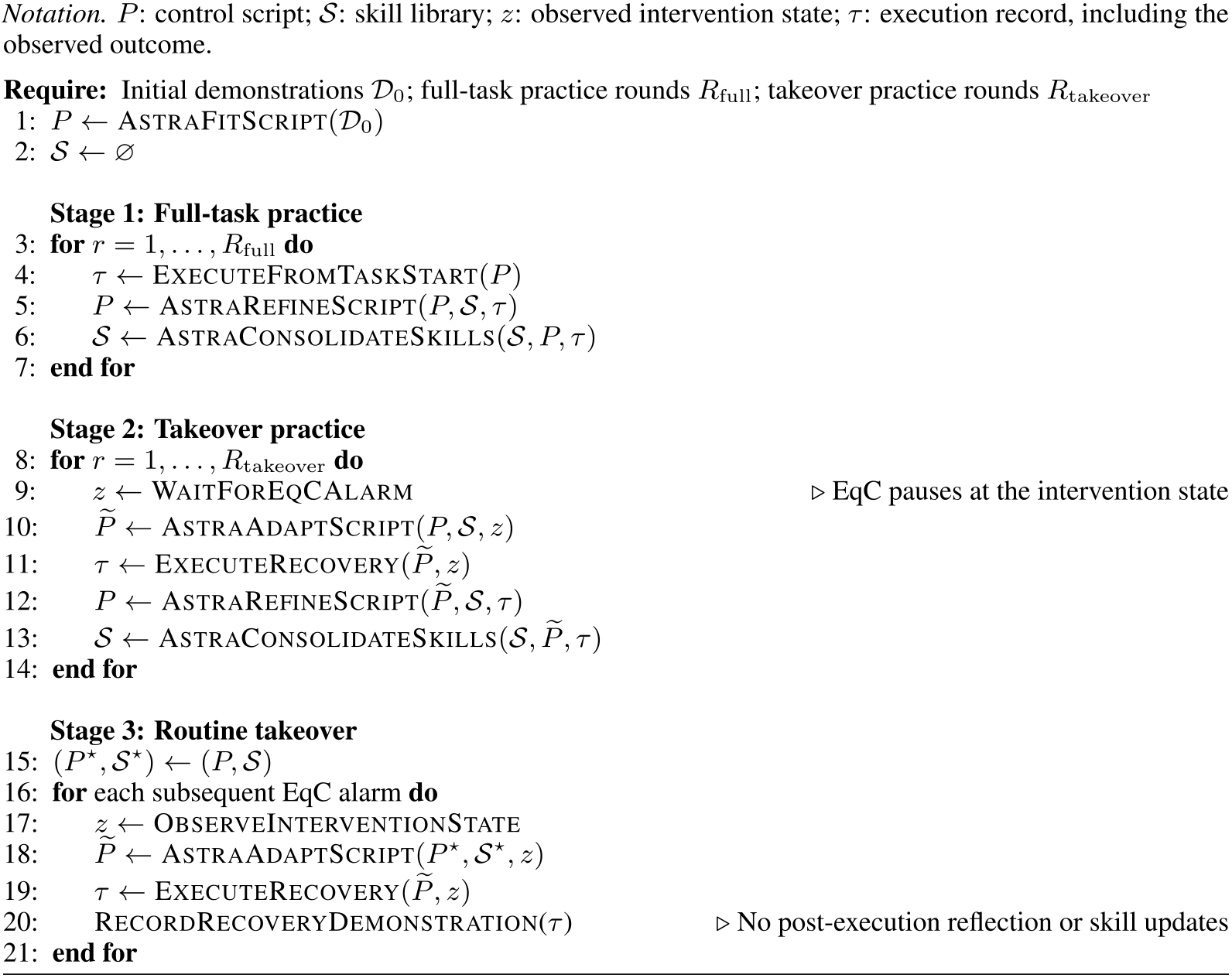
Use Run 1’s seed-trained garment checkpoint and the same γ=0.2/persistence gate. On an alarm, pause EqC and let the prepared agent adapt a recovery script to the current scene.
Expert agent preparation.
The agent studies all 18 demonstrations, writes control code, repeatedly practices full folding with revision until near-perfect success, then practices takeover from partial task states and consolidates skills. Routine takeover subsequently adapts and executes code without per-low-level-action language calls or post-execution skill updates. The number and cost of preparation attempts are not quantified, so six recoveries is not the total expert-development budget.
Takeover and policy learning.
Six routine agent recoveries are combined with the original 18 demonstrations. The updated policy completes 20/20 autonomous garment trials without takeover. This is a single-checkpoint, single-task proof of concept, separate from the three-run human-expert comparison.
Equation 74
| (74) |
Implications.
The experiment illustrates two stages of transfer: a large model’s reasoning becomes executable recovery skills, then those recoveries supervise a smaller policy. It supports automated routine collection after preparation, without demonstrating an expert-free system from scratch.
Appendix F Cross-Task Continual Learning and Catastrophic Forgetting
The cross-task study tests recovery from interference between block and cup stacking, rather than a general lifelong-learning benchmark or a forgetting-free update rule.
Protocol.
Start from the selected Run-1 stacking checkpoint at 100% block success and 0% cup success. Adding six cup recoveries yields 50% cup but drops blocks to 60%, showing actual forgetting. A further six cup and six block recoveries bring both to 100% in the reported evaluation, with 66 cumulative demonstrations. EqC helps target new and regressed skills; it does not prevent the first regression, and no multi-run cross-task comparison is supplied.
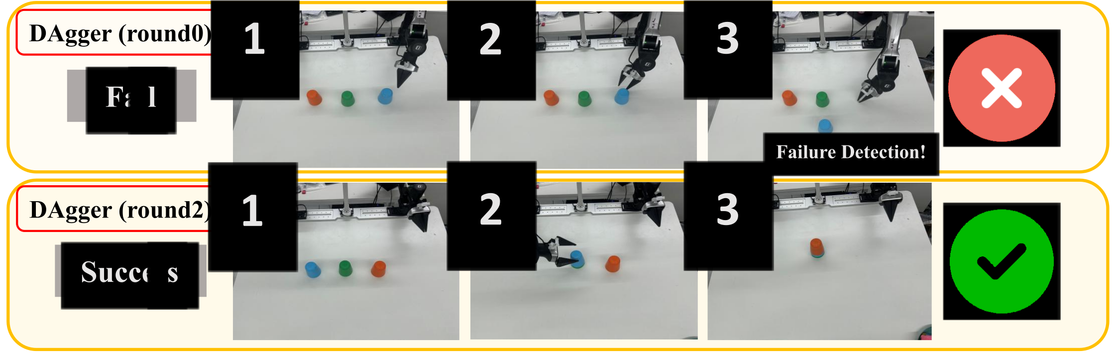
| Metric / Task | Round 0 (Base) | Round 1 (+6 Cup) | Round 2 (+6 Cup, +6 Block) |
|---|---|---|---|
| Cumulative Demos | 48 (Block only) | 54 (48 Block, 6 Cup) | 66 (54 Block, 12 Cup) |
| Block Stacking Success | 100.0 | 60.0 | 100.0 |
| Cup Stacking Success | 0.0 | 50.0 | 100.0 |
| Dual-Task Average | 50.0 | 55.0 | 100.0 |
Appendix G Ablation Study
Ablations examine step-size schedules and gradient-based early stopping. Control success and optimizer-step counts are the measured quantities; detector calibration transfer is not established by these tables.
G.1 Robustness to Optimization Step Schedules
Uniform 15-step and 20-step schedules yield 93.1% and 94.2% LIBERO success, versus 94.3% with cosine decay. This supports control robustness to these schedules. The prose extends the claim to failure detection, but Table 19 reports success rates rather than detection metrics.
| Methods | Goal | Spatial | Object | Long | Average |
|---|---|---|---|---|---|
| EqC (uniform 15 steps) | 95.8 | 95.2 | 98.4 | 83.0 | 93.1 |
| EqC (uniform 20 steps) | 95.4 | 96.2 | 98.0 | 87.2 | 94.2 |
| EqC (Cosine decay) | 95.6 | 97.2 | 98.6 | 85.4 | 94.3 |
G.2 Adaptive Inference
DiT mean gradient norm falls from 49.3 to 0.3 over 32 steps, while energy saturation reaches 99.22% at step 7 and 99.91% at step 9. Stopping below gradient 1.0 averages 16.8 steps with 93.7% success; threshold 3.0 uses 11.1 steps with 94.2%, versus 32 steps/94.0%. These are about 47.5% and 65.3% fewer refinement steps, not directly measured wall-clock savings or proof that every trajectory has converged.
| Step | |||||||||
|---|---|---|---|---|---|---|---|---|---|
| Mean Gradient Norm | 49.3 | 44.4 | 29.9 | 12.9 | 6.0 | 3.6 | 1.2 | 0.7 | 0.3 |
| Saturation Ratio (%) | 0.00 | 82.51 | 95.18 | 99.22 | 99.79 | 99.91 | 99.99 | – | – |
| Task Suite | Baseline () | ||
|---|---|---|---|
| libero_goal | / | / | / |
| libero_spatial | / | / | / |
| libero_object | / | / | / |
| libero_long | / | / | / |
| Average | / | / | / |
Appendix H Case Study: Detection Timeliness and Failure Modes
Qualitative examples show when warnings occur relative to visible execution problems. They illustrate mechanisms and failure modes, without supplying population-level rates of irreversible damage or recoverability.
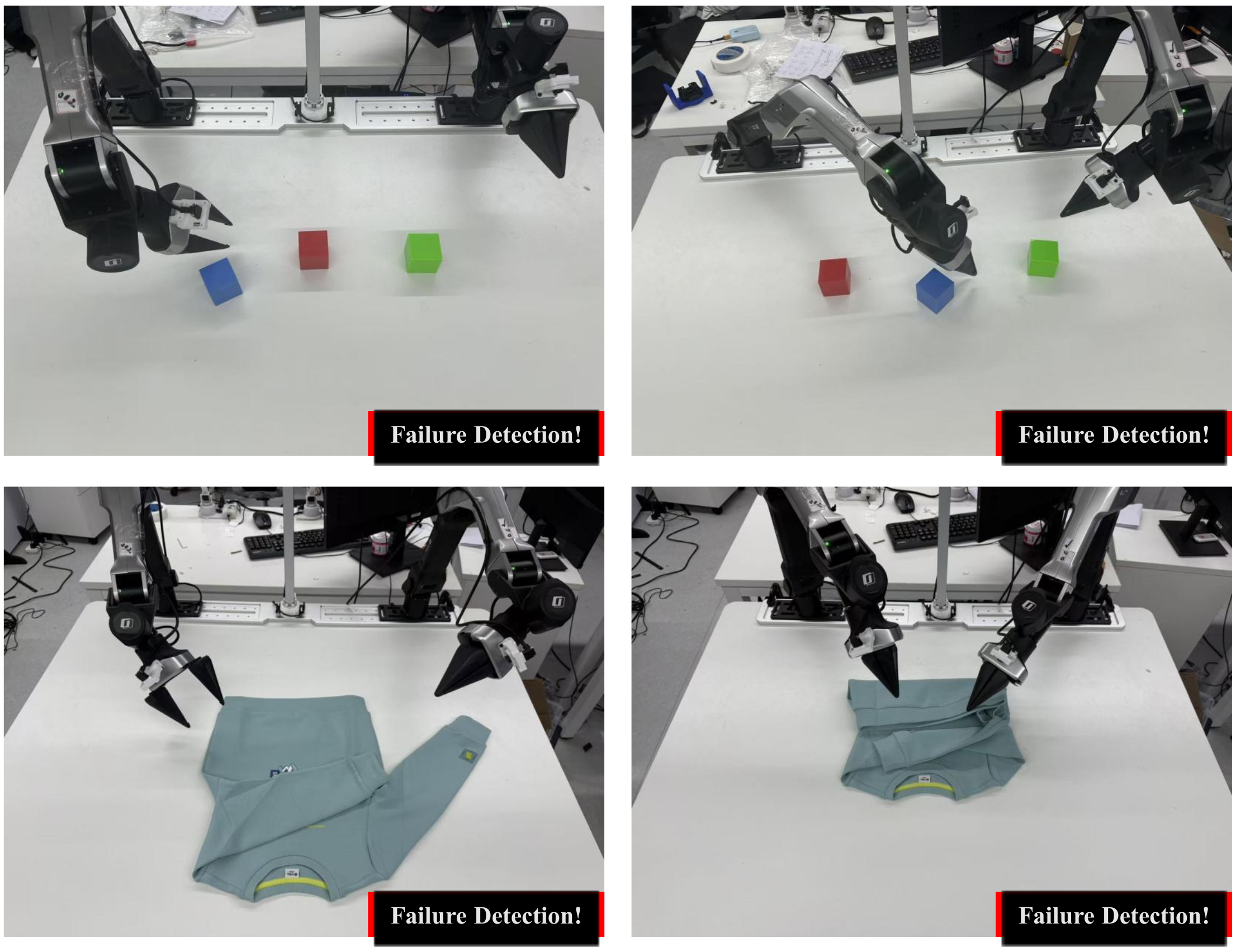
H.1 Proactive Detection by EqC at the Competence Boundary
EqC examples alarm after a displaced block, angular stacking misalignment, failed sleeve grasp or missed garment-fold target, while recovery remains possible. The original panels retain the scene and alarm labels; these selected cases complement the quantitative rollout analysis.
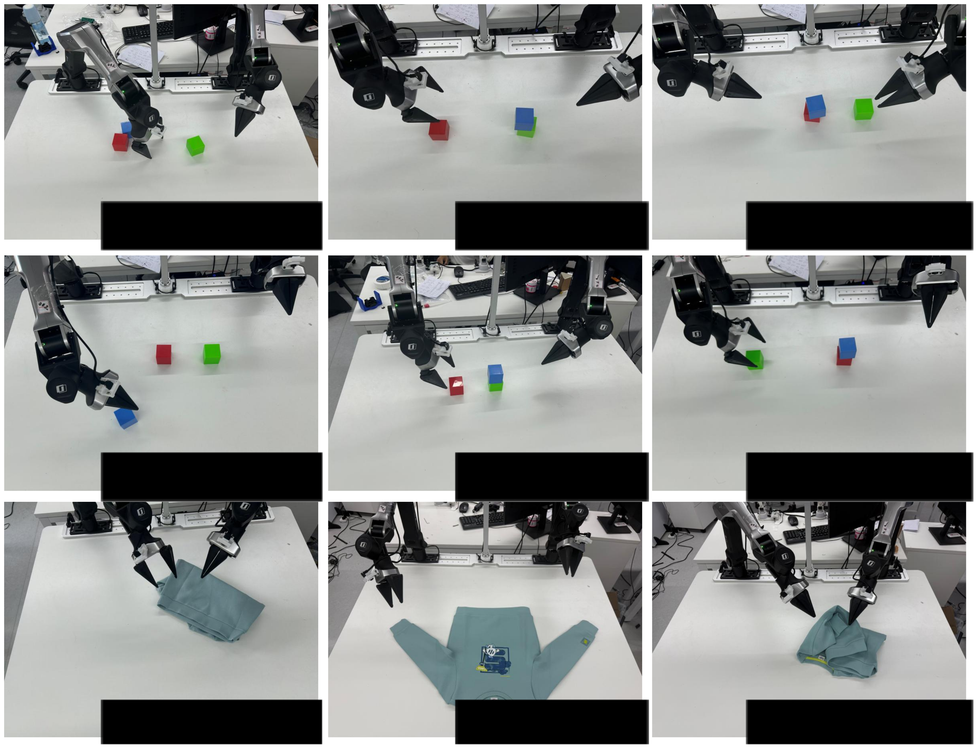
H.2 Pathology Diagnostics of Flow-Loss Detection (Diff-DAgger)
Diff-DAgger examples show delayed alarms during drift, spurious alarms in apparently competent execution, and alarms only after incorrect stacking or tangled fabric. These cases motivate earlier, more stable warnings; they do not imply that every baseline failure follows those patterns or that EqC never exhibits them.
Appendix I Code Availability
The authors link the EqC repository for implementation and evaluation procedures.