Overview
This edition covers the complete 28-page paper and supplement. The PDF’s main Figures 1–5 and supplementary Figures 1–5 remain distinct, as do the two sets of Tables 1–4. The source’s detached, flattened teaser is joined to its caption and restored from the native PDF. All original figure/table detail, equations, curation algorithm and project presentation/demonstrations remain alongside the notes. Lou and Yang contributed equally.
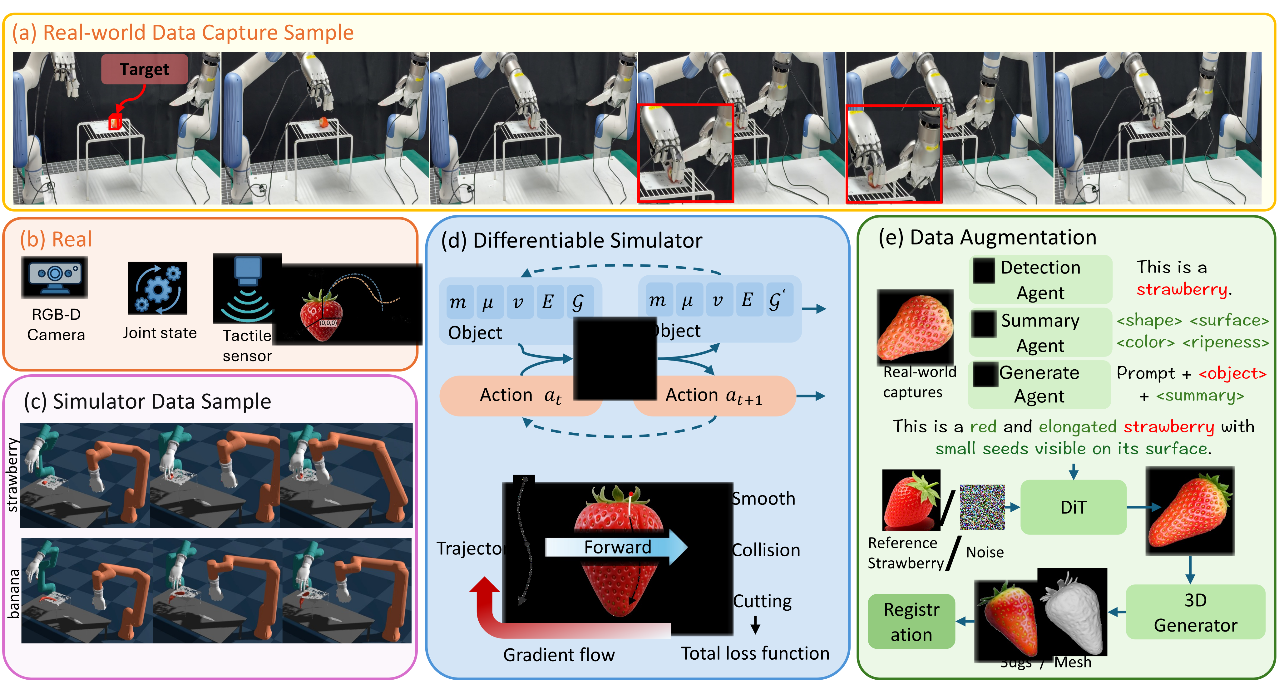
At a glance
DexNinja augments scarce real food-cutting demonstrations with reconstructed/generated assets, deformable simulation and trajectory refinement. Its main four-food experiment reaches 50/100 real cutting successes, versus 31/100 with real data alone, a 19-percentage-point gain. A separate scaling study reaches 63/100 when the reported simulated-episode budget increases to 300. Thus the abstract’s above-60% result belongs to the larger-data setting. Policies remain category-specific, with generalization tested mainly on unseen instances inside trained categories.
1 Introduction
Cutting changes material shape, contact and topology, making both repeated real collection and simulation transfer difficult. The data engine anchors new geometry/material variation to real captured examples, then admits feasible simulated rollouts. Differentiable simulation supports trajectory fitting/refinement; the deployed arm/hand policies are trained by supervised behavior cloning. The paper does not demonstrate end-to-end gradients through physical execution or one general policy for arbitrary food categories.
2 Related Works
The related work connects synthetic demonstrations, differentiable cutting and dexterous/tactile manipulation. The contribution is their combination into an anchored data-generation and deployment pipeline, rather than simulation replacing all real sensing or calibration.
2.1 Data generation and differentiable simulation
Trajectory-generation and Gaussian-splatting methods broaden motion/appearance coverage. RoboNinja, DiSECt and tactile simulators address deformable contact and cutting [8] [43] [44]. DexNinja adds reconstructed category assets, material randomization, trajectory admission and a bridge to articulated scene simulation. The implementation explicitly splits local cutting physics from the full robot engine.
2.2 Dexterous manipulation and Teleoperation
Dexterous grasping and teleoperation provide executable initial grasps and real supervision. Tactile signals help distinguish stable contact, slip and compression when visual geometry alone is insufficient. Frame alignment and sensor mapping support transfer; they do not remove embodiment-specific calibration or establish zero-shot transfer between arbitrary hands.
3 Problem Formulation
Observation combines a scene point cloud, fingertip tactile arrays and proprioception. Food parameters include mass, friction, Young’s modulus, Poisson ratio and changing geometry; the knife is a separate rigid tool. Kinematic and contact-sensitive action components are learned with separate losses. The arm branch also relies on object-centric motion specification and IK, while the hand branch responds to tactile/proprioceptive feedback. All original definitions and the elasticity conversion remain.
Equations 1–4
| (1) |
| (2) |
| (3) |
| (4) |
Equations 5–6
| (5) |
| (6) | ||||
4 Real2Sim2Real pipeline: Dexninja
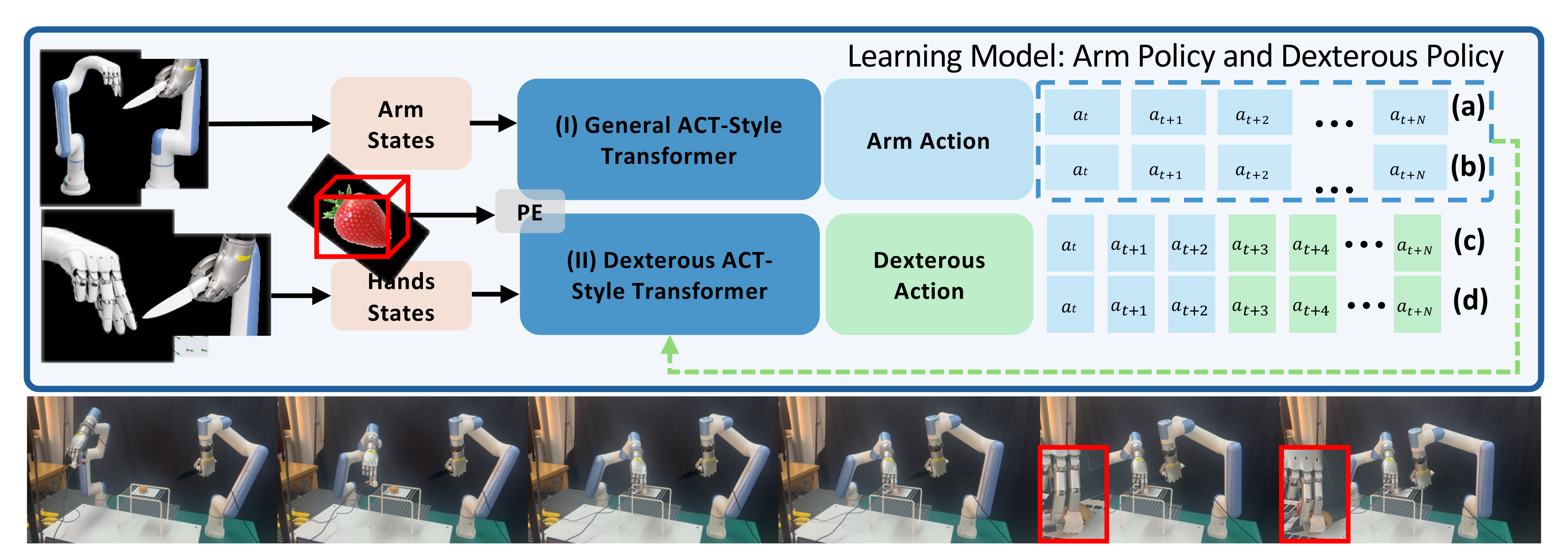
Stage I reconstructs and registers real food/tool geometry from synchronized teleoperation. Stage II varies assets/materials, refines knife trajectories, solves IK and filters rollouts through collision/cutting checks. Stage III clones the accepted multimodal trajectories with separate arm/hand heads. A stage token controls chunk horizons: nominal 64 for approach/grasp, 128 for knife positioning and 16 for contact-rich cutting. These are step counts; the paper does not supply a common control frequency that would turn them into fixed durations.
Equations 7–8
| (7) |
| (8) |
5 Continuation on a Shape Manifold for Data Augmentation
The augmentation section describes category-conditioned shape variation and local correction around successful examples. Its mathematical shape-manifold/continuation view is a local modeling argument. Practical generation uses descriptions, image cleaning, image-to-3D and multiple admission checks; semantic plausibility alone is not treated as physical cutting feasibility.

Data augmentation pipeline
A detector identifies the food category and a summary extracts shape, surface, color and ripeness attributes. Text/image/3D generation diversifies those attributes while remaining anchored to captured examples. Geometric and simulator checks then decide which assets and trajectories enter training. The pipeline does not claim every language-generated instance is automatically a valid physical material.
Shape generation and local manifold structure
A latent generator G formalizes a local family of category shapes. The stated assumption is local regularity, with a locally Lipschitz generator offered as sufficient. The paper does not measure a certified smooth neighborhood for every generated asset. The implementation’s curated image-to-3D pool is evidence of useful variation, rather than a proof that all assets lie on a known smooth manifold.
Equation 9
| (9) |
Local regularity and analytical reliability
A first-order expansion of the visual-to-action map motivates small corrections near a successful anchor. Local Lipschitz behavior requires suitable local smoothness/bounded derivative assumptions; differentiability at one point alone is insufficient for the stated neighborhood bound. The argument also does not guarantee task success across contact/topology changes. Empirical simulation admission is still required.
Equation 10
| (10) |
Neighborhood of demonstrations
The formal local corrective policy maximizes simulated feasibility while penalizing departure from the demonstrated action. State, shape and material perturbations define the neighborhood distribution. This expresses how continuation should remain near successful behavior. The supplement concretely describes trajectory optimization and filtering, without a complete optimizer/architecture specification for each per-anchor corrective policy in the formal equation.
Equation 11
| (11) |
Augmented data generation
Augmented pairs are retained only after successful simulated outcomes. This biases the training pool toward demonstrated-neighborhood feasibility rather than arbitrary perturbations. It also means rejected samples and uncovered recovery modes are not automatically learned; later real failures reveal remaining grasp/contact and material-model gaps.
Equation 12
| (12) |
Real-world anchoring and admission
Plausibility is operational: semantic/multi-view consistency, scale, valid geometry, simulator compatibility and stable initialization. Rollouts additionally pass IK, collision and cutting-success checks. Randomized mass/friction/elasticity stay category-bounded, although full numerical ranges and every admission threshold are not provided in the manuscript.
6 Experimental Evaluation
Real evaluation distinguishes reaching contact, completing a cut and preserving food integrity. It tests different training sources, selected longer-horizon examples and matched-budget component removals. The main quantitative results use the primary embodiment; the second setup supplies qualitative verification.
6.1 Task setup and evaluation protocol
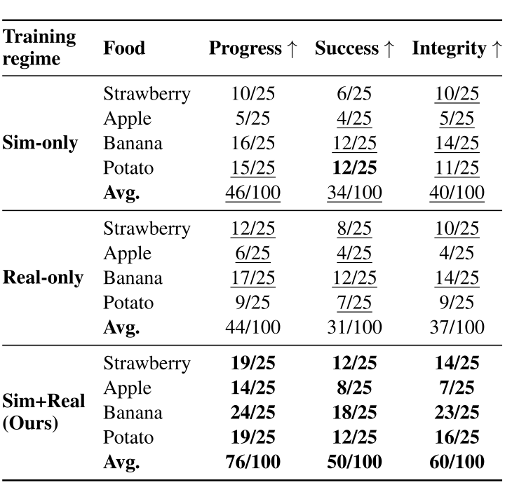
Four categories—strawberry, apple, banana and potato—have 25 held-out instances each. The stated training protocol uses five real demonstrations and fifty simulated sequences, with a separate scaling study. Progress reaches valid initial cutting contact; Success completes traversal/separation and termination; Integrity is a manual binary damage judgment. The three counts are reported separately, without their joint success-and-integrity rate. Random planar placement remains inside a reachable workspace; numerical placement bounds and rater reliability are not specified.
Accessible table and original citation links
|
Training regime |
Food | Progress | Success | Integrity |
| Sim-only | Strawberry | 10/25 | 6/25 | 10/25 |
| Apple | 5/25 | 4/25 | 5/25 | |
| Banana | 16/25 | 12/25 | 14/25 | |
| Potato | 15/25 | 12/25 | 11/25 | |
| Avg. | 46/100 | 34/100 | 40/100 | |
| Real-only | Strawberry | 12/25 | 8/25 | 10/25 |
| Apple | 6/25 | 4/25 | 4/25 | |
| Banana | 17/25 | 12/25 | 14/25 | |
| Potato | 9/25 | 7/25 | 9/25 | |
| Avg. | 44/100 | 31/100 | 37/100 | |
|
Sim+Real (Ours) |
Strawberry | 19/25 | 12/25 | 14/25 |
| Apple | 14/25 | 8/25 | 7/25 | |
| Banana | 24/25 | 18/25 | 23/25 | |
| Potato | 19/25 | 12/25 | 16/25 | |
| Avg. | 76/100 | 50/100 | 60/100 |
6.2 Sim-to-real gap and the effect of mixing sim and real data
Across 100 trials per training regime, sim-only gives 46% progress, 34% success and 40% integrity; real-only gives 44/31/37%; mixed data gives 76/50/60%. The mixed success gain over real-only is 19 points, or about 61% relative. Gains are uneven: mixed success is 12/25 strawberry, 8/25 apple, 18/25 banana and 12/25 potato. Apple has eight cutting successes but seven integrity passes, underscoring the separately reported criteria. None of these marginal counts supplies a joint damage-free success rate.
6.3 Complex Motion and Heterogeneous Objects
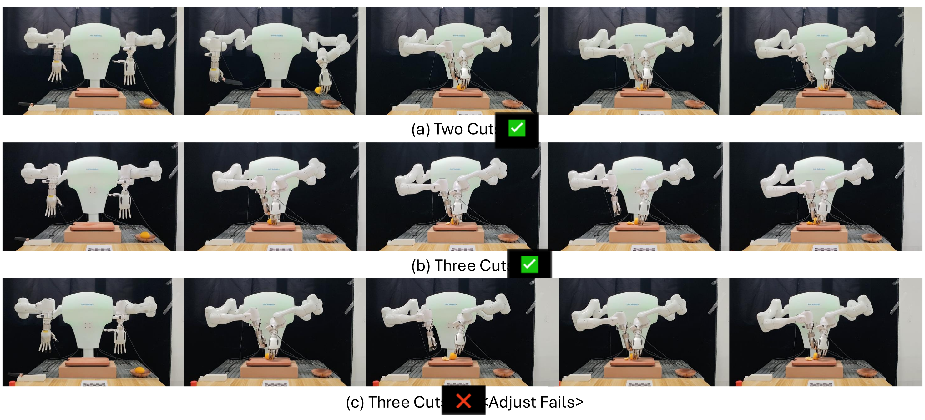
Lemon trials score 8/10 single-cut, 7/10 two-cut and 3/10 multi-cut. More cuts require repeated adjustment while geometry and contact evolve. The paper says training details follow the main protocol; it does not establish that lemon performance is zero-shot transfer from the four original category policies. The selected videos/filmstrips illustrate behavior and failure, rather than adding to those trial counts.

6.4 Component ablations and failure analysis
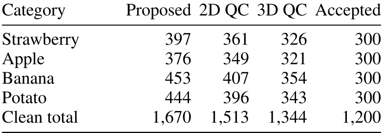
Matched-budget removals lower success from 50% to 46% without QC, 44% without material randomization, 39% without trajectory refinement, 43% without tactile observation and 42% without generated assets. Tactile removal has the largest integrity drop, 60→45%. The fifty failed mixed-data trials receive one earliest-cause label: eight registration, nineteen grasp/contact, seventeen material-physics mismatch and six kinematic/collision. These are assigned failure categories, not independent causal effect estimates. Asset curation keeps 1,200 from 1,670 proposals through successive checks.

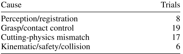
Accessible table and original citation links
| Cause | Trials |
| Perception/registration | 8 |
| Grasp/contact control | 19 |
| Cutting-physics mismatch | 17 |
| Kinematic/safety/collision | 6 |
7 Conclusion
The engine combines real anchoring with simulated geometric/material diversity and accepted trajectory supervision. Evidence supports better within-category cutting transfer than either single data source in the reported setup. It leaves substantial real failures and more difficult multi-cut adjustment unresolved.
8 Limitations
The mounted camera constrains deployment, and current policies are object/category-specific. New categories require new assets and retraining or fine-tuning. Cross-embodiment evidence is qualitative, with calibration/kinematics/action scaling replaced for the new system.
Acknowledgments
The acknowledgment names a vivo–INSAIT collaboration and Bulgarian Ministry of Education and Science support. The full 88-reference bibliography remains, with links from the notes and retained tables.
Original project presentation and demonstrations
The primary DexNinja project supplies an unchanged narrated presentation and three unchanged physical demonstrations, all preserved with original posters. Strawberry/banana clips are labeled 4× speed and the second-setup lemon clip 8×. The original presentation chapter guide is 0:00 Motivation, 0:30 Pipeline, 2:00 Policy learning, 2:30 Experiments and 4:12 Deployment. These are selected demonstrations, rather than extra trials to add to the paper’s success counts.
Supplementary Material
The complete supplement covers local cutting simulation, scene registration, policy training, hardware, asset curation, additional quantitative experiments and qualitative executions. Its equation and figure numbering restarts independently of the main text.
1 Simulation Details
Simulation transfers a demonstrated knife motion through explicit world, food, knife and end-effector frames. Local cutting physics supplies contact information, while scene-level kinematics handle the articulated robot. The bridge is important because the chosen robot engine does not natively support the required food cutting dynamics.
1.1 Stage I: Teleoperation and Object Frame
A successful demonstration records synchronized sensor/action streams and estimated food pose. Expressing the knife trajectory in the food frame removes its original world placement. This canonical blade/object relation is retargeted to reconstructed instances; it still requires estimating object pose and the grasp transform accurately.
Equation 1
| (1) |
1.2 Stage II: Differentiable Cutting Simulator Details
A fixed end-effector/knife transform maps perturbed object-frame knife paths into world-frame robot targets. IK filters joint-space realizations before simulation generates aligned observations/actions. The rigid-grasp transform assumes the knife does not slip in the hand; tool-grasp failures are part of the remaining transfer challenge.
Equations 2–3
| (2) |
| (3) |
Trajectory generation loss.
The differentiable objective samples blade points and uses ground SDF distance, weighted progress, penetration, rotation and motion-consistency terms. Positive SDF is outside the ground. The nonnegative tolerance m permits small numerical penetration; it is not a required positive clearance. The distance-to-ground cutting proxy helps refine paths, while successful material separation is separately checked through the rollout predicate. The complete loss formulas remain, including all averaging and weighting terms.
Equations 4–11
| (4) |
| (5) |
| (6) |
| (7) |
| (8) |
| (9) |
| (10) |
| (11) |
1.3 Tactile Simulation During Cutting
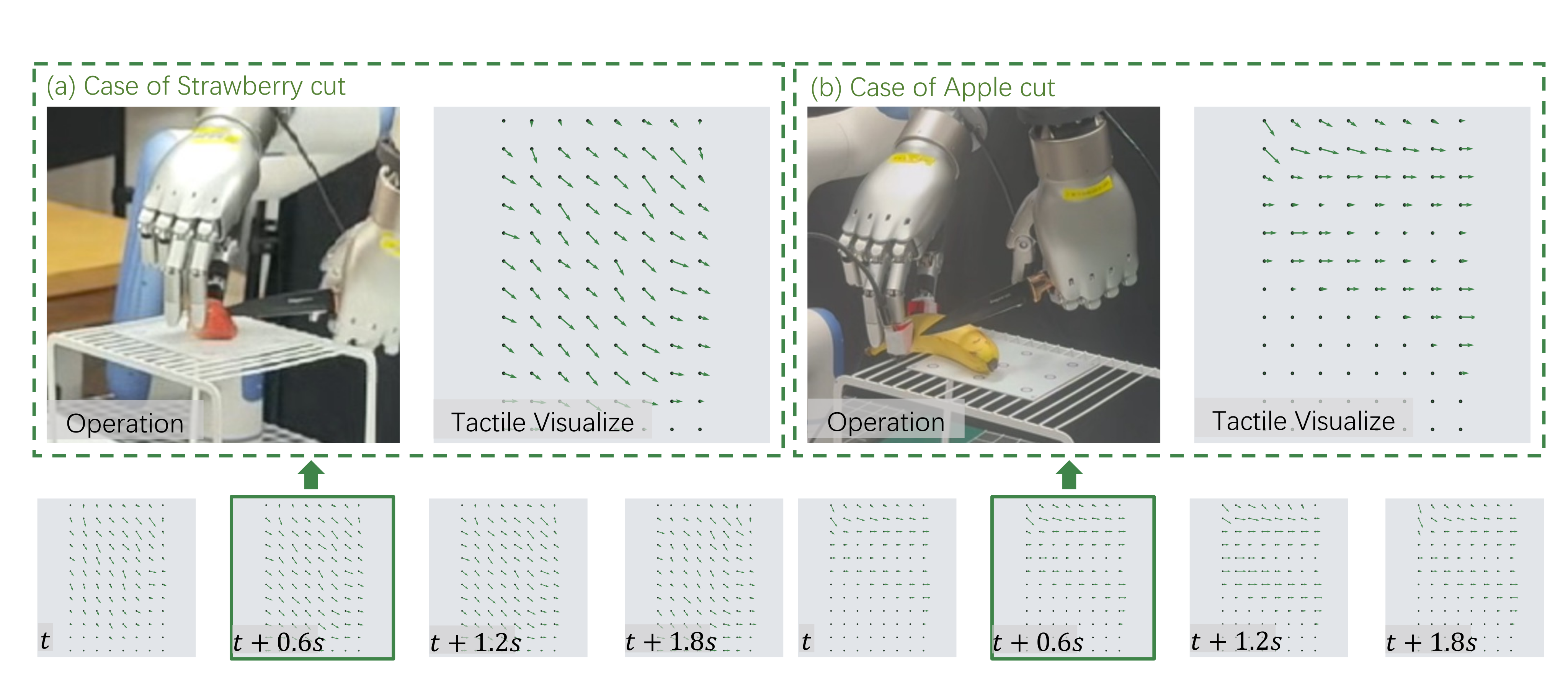
A grasp prior initializes the stabilizing hand. The MPM cutting layer estimates particle/sensor contact forces from penetration and relative tangential motion, bins them spatially and applies small finger corrections when slip is indicated. Those simulated corrections become supervision. Contact positions/directions are expressed in the active tool/end-effector frame, with a scale/offset/noise mapping to real readings. This is model-based synthetic tactile feedback, with residual mismatch reflected in real failures.
1.4 Scene level and hardware registration
Canonical targets are registered to the scene and converted through IK/time parameterization with motion limits. Stabilization precedes the knife motion on a shared timeline. The local deformable simulator passes knife pose, contact points and forces/moments or a net wrench to the articulated scene simulator. This modular bridge supplies consistent interaction information; the paper does not describe a single monolithic robot/food solver or certify every transferred contact outcome.
2 Training Details
The final supervised policy retains multimodal observations and separate kinematic/contact action groups. The curriculum first reaches reliable pre-contact configurations, then uses tactile feedback during cutting. Its training description includes normalized chunk prediction and executed-increment smoothing, rather than a full real-world reinforcement-learning objective.
Equation
Why a single globally normalized action head is unstable.
Finger and arm actions have different ranges, so one output normalization can make hand motion dominate training or leave it under-actuated. Separate heads and group/stage statistics address that scaling problem. The later ablation measures the concrete head design, without proving every universal-head architecture must fail.
2.1 Stage-conditioned action chunking
Stage labels are approach/grasp, knife positioning and tactile cutting. A two-sided uniform mixture samples horizons around their 64/128/16 nominal values during post-training. At inference the stage is determined by geometry/contact rules. The manuscript leaves exact horizon bounds and mixture weights unspecified, so the complete stochastic execution schedule cannot be reconstructed from the nominal values alone.
Equations 12–13
| (12) |
| (13) |
2.2 Group-wise action normalization and execution
Targets use group- and stage-specific clipped z-scores. Execution maps normalized outputs to scaled joint increments, then projects into a robot-specific command set. Arm steps are described as smaller than hand steps. Numerical step sizes and the full projection implementation are not provided. This is the stated command mapping rather than simply undoing the target z-score; the original equations preserve that distinction.
Equations 14–16
| (14) |
| (15) |
| (16) |
2.3 Chunked behavior-cloning objective
Chunk behavior cloning sums stage-weighted arm and tactile L1 errors over the sampled horizon. A rate penalty regularizes changes in consecutive executed increments. Arm weighting is larger during approach/positioning; tactile weighting rises during cutting. Complete optimizer, model-width and loss-weight tables are not supplied for exact reproduction.
Equations 17–18
| (17) |
| (18) |
2.4 Sim2Real deployment
Stage switching uses knife proximity and tactile onset. Lost contact for a fixed number of steps returns the system to knife positioning, with lower off-threshold than on-threshold to create hysteresis. All commands pass the stated joint/rate/workspace/collision filter. These mechanisms aid execution but are not a whole-task success or physical damage guarantee.
Equations 19
| (19) |
3 Implementation Details
The implementation distinguishes algorithmic representation from hardware-specific execution. Both platforms use object-centric blade motion and tactile hand regulation, while transforms, IK, joint limits and action scales adapt to the robot.
3.1 Two-Embodiment Setup Verification
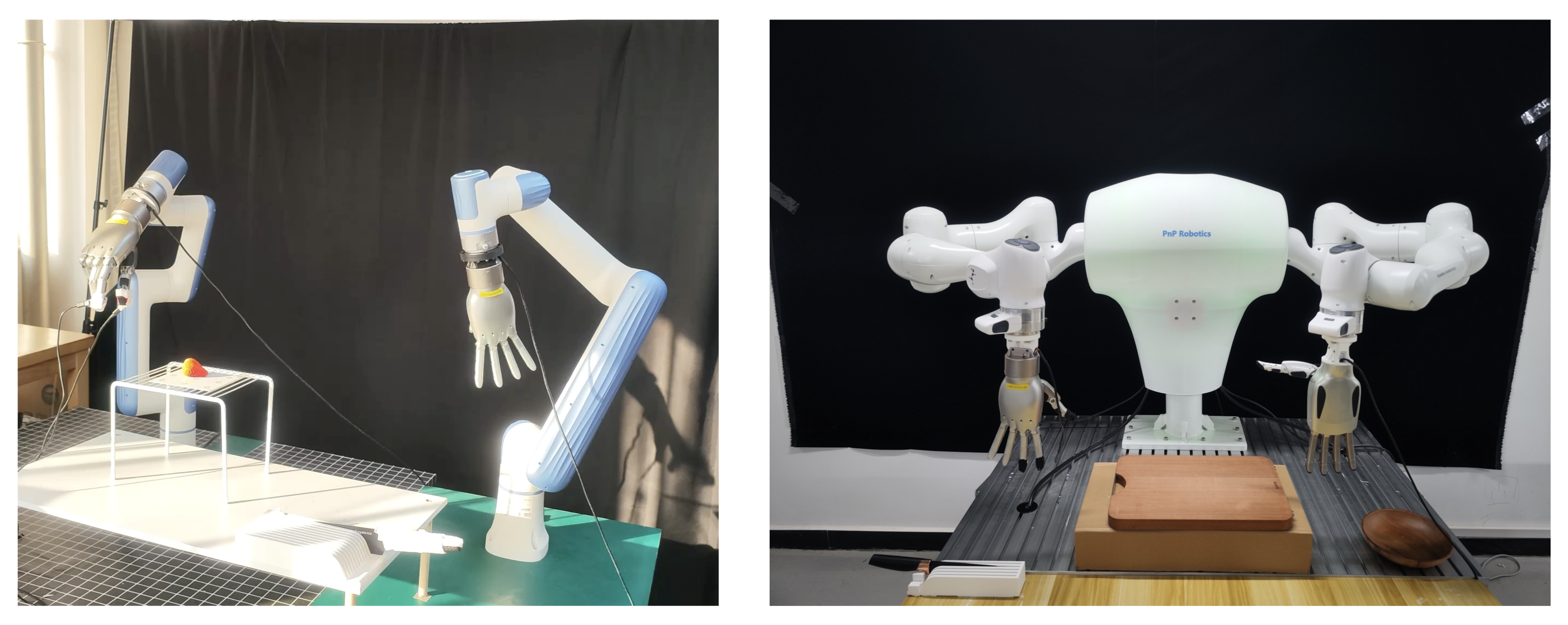
The source identifies the main platform as DR3/DR5 arms with LinkerHand L10 hands and an Orbbec 435Le camera. The second uses dual Franka arms and LinkerBot L20 hands with recalibrated vision. Main quantitative trials belong to the first; the second is a qualitative morphology-shift check. No matched second-platform success table or proof of unchanged learned-weight transfer is supplied.
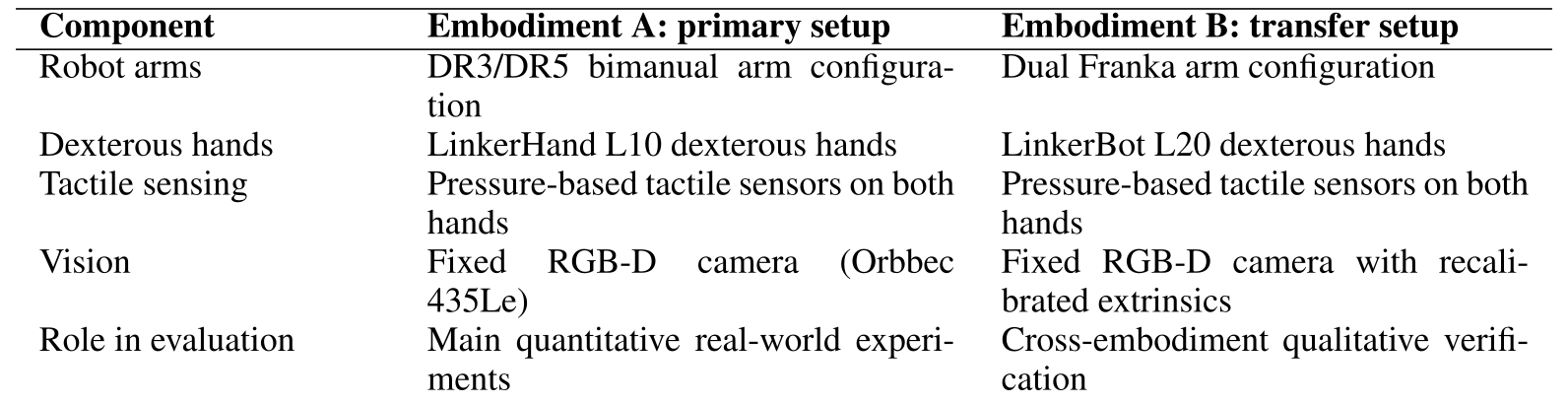
Accessible table and original citation links
| Component | Embodiment A: primary setup | Embodiment B: transfer setup |
| Robot arms | DR3/DR5 bimanual arm configuration | Dual Franka arm configuration |
| Dexterous hands | LinkerHand L10 dexterous hands | LinkerBot L20 dexterous hands |
| Tactile sensing | Pressure-based tactile sensors on both hands | Pressure-based tactile sensors on both hands |
| Vision | Fixed RGB-D camera (Orbbec 435Le) | Fixed RGB-D camera with recalibrated extrinsics |
| Role in evaluation | Main quantitative real-world experiments | Cross-embodiment qualitative verification |
3.2 Embodiment-Specific Control and Safety Filters
Normalized outputs are scaled and projected for each robot. Knife targets violating collision/limit/singularity checks are discarded or repaired. Filtered tactile control runs slower than arm pose tracking, but numerical rates are not reported. The separation supports modular deployment while leaving a substantial robot-specific execution layer.
Equations 20–21
| (20) |
| (21) |
4 Knowledge-Guided Data Augmentation
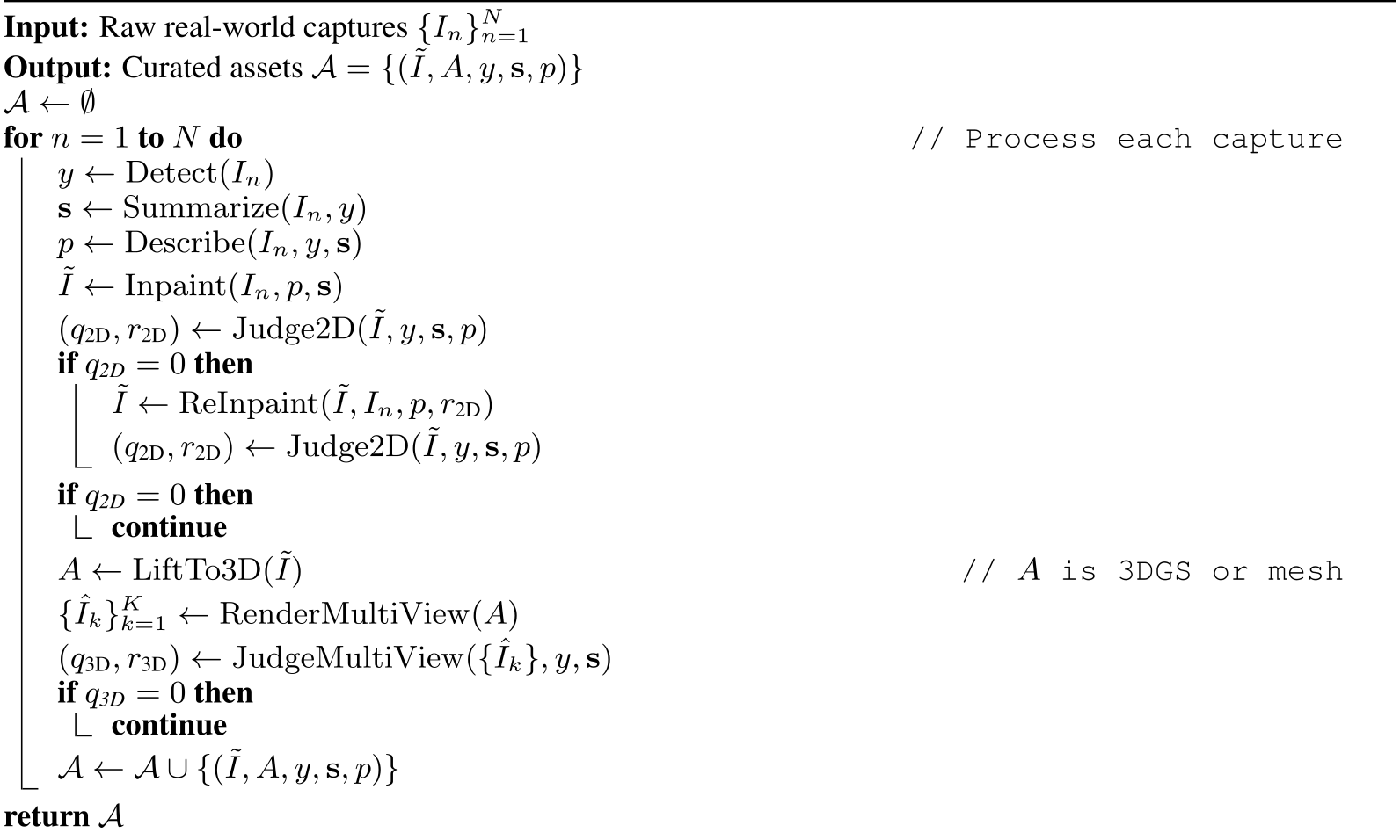
Knowledge-guided curation turns captured references into clean single-object images and validated 3D assets. Algorithm 1 retains detection, description, reinpainting, multi-view judgment and rejection branches. Visual admission is followed by physical initialization and successful-trajectory checks.
Inputs
Inputs can contain clutter or occlusion. A detector predicts category and a summary records shape/surface/color/ripeness descriptors. The structured attributes condition later generation and judge consistency; they are not direct measurements of mass, friction or elastic constants.
Template-constrained description synthesis
A constrained description template orders the extracted attributes, improving controllability across later generators. The original example is “This is a <adj> <object> with <features>”. The source supplies this example and algorithmic roles, rather than full model-specific prompt transcripts.
Equation
Image cleaning via inpainting and transparency
Inpainting aims for one centered object without hands/tools/clutter and with transparency. Attribute preservation is checked later rather than assumed from generation alone. Clean appearance assets still require scale/geometry and physical admission before simulation use.
Equation
Automatic quality control (QC) for 2D
A vision-language judge checks category/attribute match, transparency, single-object composition and artifacts. Failed images may be reinpainted with rejection reasons; persistent failures are discarded. This is the implemented QC route, not a certified error-free semantic verifier.
3D asset generation and multi-view validation
An image-to-3D model such as Trellis produces a Gaussian-splatting or mesh asset [88]. Rendered views are judged for identity, geometry and texture stability. Passing assets then face simulator compatibility and initialization checks; successful cutting/IK/collision checks apply at rollout level.
Outputs
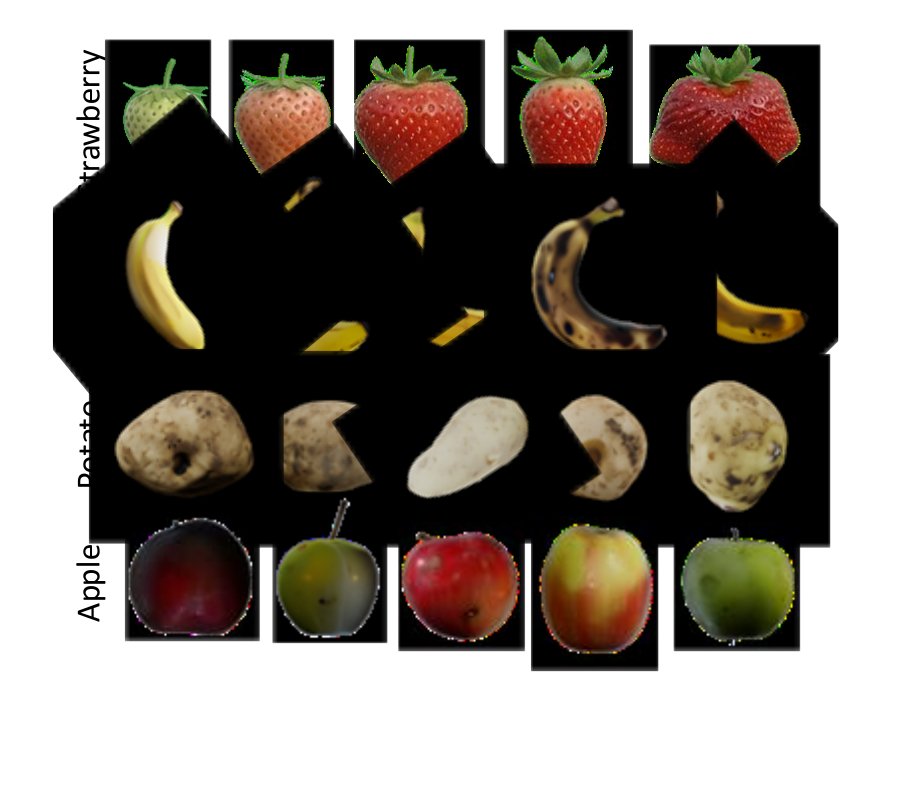
Each retained item stores its transparent image, 3D representation, category, attribute record and description. The illustrated pool spans the four training food categories. It broadens an anchored empirical neighborhood without establishing a guaranteed continuous latent manifold of executable behaviors.
Equation
Original selectable algorithm
5 Additional Experiments
Additional studies compare a reproduced cutting baseline, scale simulated data, ablate policy organization and inspect pressure regulation. Their protocols and denominators differ from the main hundred-trial study; their success rates should remain attached to their own tables.
5.1 Comparison to baseline
Over forty trials, DexNinja scores 23/40 (57.5%) and the RoboNinja reproduction 12/40 (30.0%), a 27.5-point aggregate gain. It improves strawberry/potato/banana but loses on apple, 3/10 versus 7/10. This comparison is a separate ten-per-category experiment, not the main 25-per-category result.

Accessible table and original citation links
| Method | Strawberry | Potato | Banana | Apple | Avg. |
| RoboNinja (baseline) | 1/10 | 2/10 | 2/10 | 7/10 | 12/40 |
| Ours | 6/10 | 5/10 | 9/10 | 3/10 | 23/40 |
Baseline implementation.
The baseline keeps RoboNinja’s rigidly attached knife assumption, while DexNinja grasps the tool dexterously. Original force-sensor details could not be recovered, so contact feedback is approximated from tactile readings. The authors explicitly qualify it as a protocol-matched reproduction with an approximate sensing interface. It is not a fully exact recreation of the original hardware/controller.
5.2 Simulation scaling and generation cost
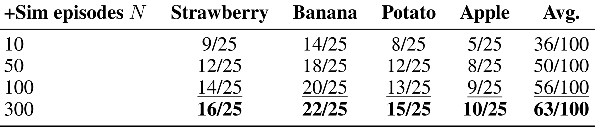
With real data fixed, adding 10/50/100/300 simulated episodes gives 36/50/56/63 successes out of 100. This is an observed data-scaling trend, rather than a fitted universal scaling law. Generation costs are substantial: about ten minutes and 20 GB GPU memory per single-cut episode on an H200, before parallelization. The source estimates N·M/6 GPU-hours and roughly 10+10M GB memory for N episodes of M cuts, excluding other pipeline/training costs.
Accessible table and original citation links
| +Sim episodes | Strawberry | Banana | Potato | Apple | Avg. |
| 10 | 9/25 | 14/25 | 8/25 | 5/25 | 36/100 |
| 50 | 12/25 | 18/25 | 12/25 | 8/25 | 50/100 |
| 100 | 14/25 | 20/25 | 13/25 | 9/25 | 56/100 |
| 300 | 16/25 | 22/25 | 15/25 | 10/25 | 63/100 |
5.3 System-level ablations
The forty-trial head/chunk study scores 11/40 with a universal head, 21/40 with separate heads, 13/40 with fixed horizon 64 and 24/40 for the full system. The full design has the best aggregate count, with task-level ties. Small ten-per-category samples and missing training-seed intervals limit fine-grained ranking; the table supports this implementation’s organization rather than all possible head designs.

Accessible table and original citation links
| Object | Universal Head | Separate Heads | Fixed Action Chunk | Full System |
| Apple | 2/10 | 4/10 | 1/10 | 5/10 |
| Banana | 4/10 | 7/10 | 6/10 | 7/10 |
| Strawberry | 2/10 | 5/10 | 2/10 | 7/10 |
| Potato | 3/10 | 5/10 | 4/10 | 5/10 |
| Average | 11/40 | 21/40 | 13/40 | 24/40 |
5.4 Tactile regulation versus forceful grasping
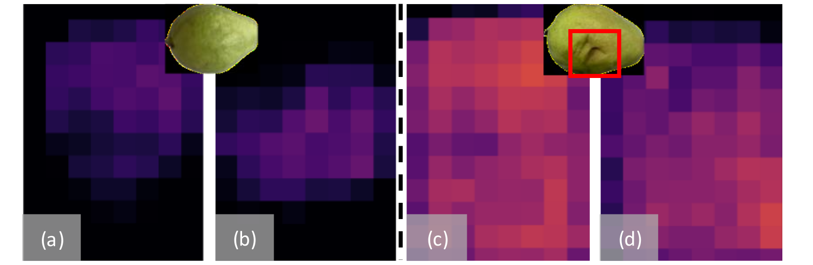
A guava example contrasts localized contact with broader activation and visible compression at high force. It illustrates the tradeoff between slip and over-compression. It is qualitative evidence of why regulation matters, not a quantified guarantee that the policy always stays inside a measured safe contact envelope.
5.5 Summary of additional findings
The combined evidence supports useful data densification and separate/stage-conditioned control, with unequal gains by category. Additional simulation raises success but remains costly, and no experiment eliminates the grasp, material-model or long-horizon adjustment failures.
6 Qualitative Results
Full qualitative filmstrips retain primary and second-platform executions, food-specific colors, multiple cuts and adjustment failure. Selected successful sequences complement the complete trial tables without changing their denominators.
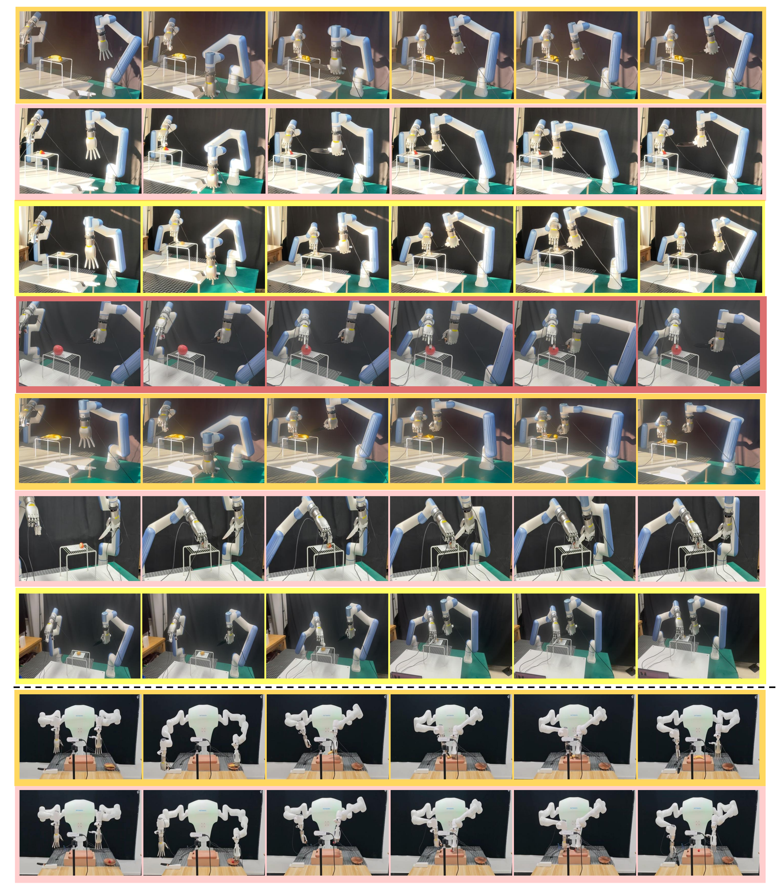
Knife initialization and handover.
DexGraspNet 2.0 proposes knife-handle grasps and pre-grasp configurations before the policy takes over [87]. This standardizes tool starting pose and clearance. It is an initialization prior, rather than evidence that the learned cutting policy autonomously acquires an arbitrary tool from arbitrary initial configurations.
Multi-cut Experiment Results.
Two cuts largely repeat the single-cut interaction. Three cuts require fruit adjustment and realignment, where accumulated pose/contact errors cause additional failures. The full supplementary Figure 5 includes both successful three-cut execution and a failed adjustment, preserved with their labels.
Phase structure in real rollouts.
Selected rollouts show approach, contact initiation and progressive slicing with small pose corrections. The narrative describes how soft banana, delicate strawberry and resistant potato differ. These observations characterize examples; they do not add a controlled per-material mechanism experiment or a calibrated material estimator.
Common qualitative failure modes.
Observed failures include initial misalignment, premature contact, late jamming/friction and unsuccessful multi-cut realignment. Three-cut adjustment is especially sensitive to accumulated disturbance. These examples are consistent with the main failure counts and show the remaining limits of the learned data distribution.