Overview
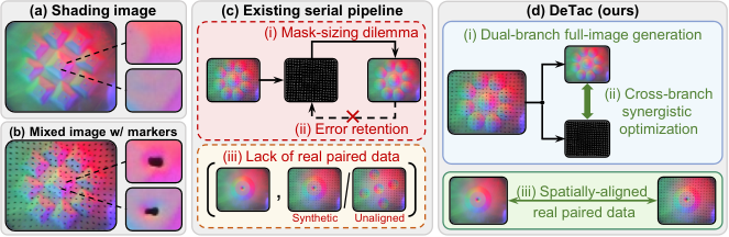
DeTac separates an optical tactile image into restored surface shading and a marker map, with complete supplementary network, dataset, and fabric-classification details retained below.
At a glance
Embedded tactile markers obscure surface appearance and also deform nearby elastomer, so removing only the visible dots leaves geometric artifacts. DeTac combines a full-image diffusion restorer with a lightweight marker predictor, trained jointly on physically aligned before/after-marker contacts. The separated outputs improve the tested surface-reconstruction and force-estimation pipelines. These are inferred appearance and marker representations; force and geometry still require downstream models. Sequential diffusion sampling limits real-time use.
1 Introduction
Markerless optical sensors reveal contact shape through illumination, whereas marker displacement supplies cues for force estimation. Combining them in one image creates both occlusion and indentation around the markers. A fixed inpainting mask may miss these surrounding changes or erase useful texture if enlarged. DeTac addresses this with whole-image restoration, coupled marker prediction, and real paired contacts, rather than treating markers as an independently pasted overlay.
2 Related Work
Related work motivates both the tactile hardware problem and conditional image-generation design.
2.1 Vision-based Tactile Sensors
GelSight, GelSlim, DIGIT, and TacTip use different marker fabrication methods, but each can couple marker appearance with surface geometry. UVTac [17] separates modes through switchable illumination at added hardware cost. DeTac instead estimates both components from one observation. Its training setup uses the MC-Tac sensor [52] with a mechanical contact-alignment fixture.
2.2 Conditional Image-to-image Generation
Masked inpainting generates only selected regions, while conditional full-image models can also correct nearby shading. DeTac adopts the latter because indentation extends beyond visible marker pixels. Diffusion offers a flexible conditional image model but adds iterative inference; the experiments therefore also compare deterministic paired-data regressors to separate representation quality from the choice of generative backbone.
3 Method
The method defines simultaneous shading and marker prediction, two losses linking their spatial structure, and a hardware-assisted paired-data procedure.
3.1 Concurrent Dual-Branch Prediction
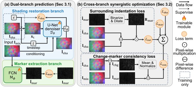
A conditional U-Net follows the denoising diffusion formulation [18]: it receives the mixed tactile image, a noisy clean-image target, and a timestep, learns to predict noise, and reconstructs shading through iterative denoising from Gaussian noise. It can modify the whole image, including marker neighborhoods. The complete forward-noising, clean-estimate, loss, and reverse-sampling equations are retained.
A separate three-layer convolutional branch produces a soft marker map in one deterministic pass. Binary cross-entropy supervises its output against pseudo-labeled marker masks. Soft boundaries accommodate defocus. Marker centroids and displacements can then feed a force estimator, but the marker branch itself does not output calibrated forces.
Equations 1–6
| (1) |
| (2) |
| (3) |
| (4) |
| (5) |
| (6) |
3.2 Cross-Branch Synergistic Optimization
The surrounding-indentation loss focuses shading error on a narrow ring formed by dilating thresholded predicted markers and subtracting their interiors. The consistency loss compares the predicted marker map with a normalized, squared difference between mixed and restored images. This encourages marker locations and restoration changes to agree, supplementing imperfect segmentation labels.
The joint objective combines diffusion, marker, surrounding-region, and consistency terms. Auxiliary losses start only after one hundred epochs to reduce instability from initially poor predictions. The construction encodes an association between appearance changes and markers; the quantitative ablations test its usefulness rather than proving uniquely identifiable physical separation.
Equations 7–11
| (7) |
| (8) |
| (9) |
| (10) |
| (11) |
3.3 Real-World Paired Dataset Collection
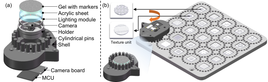
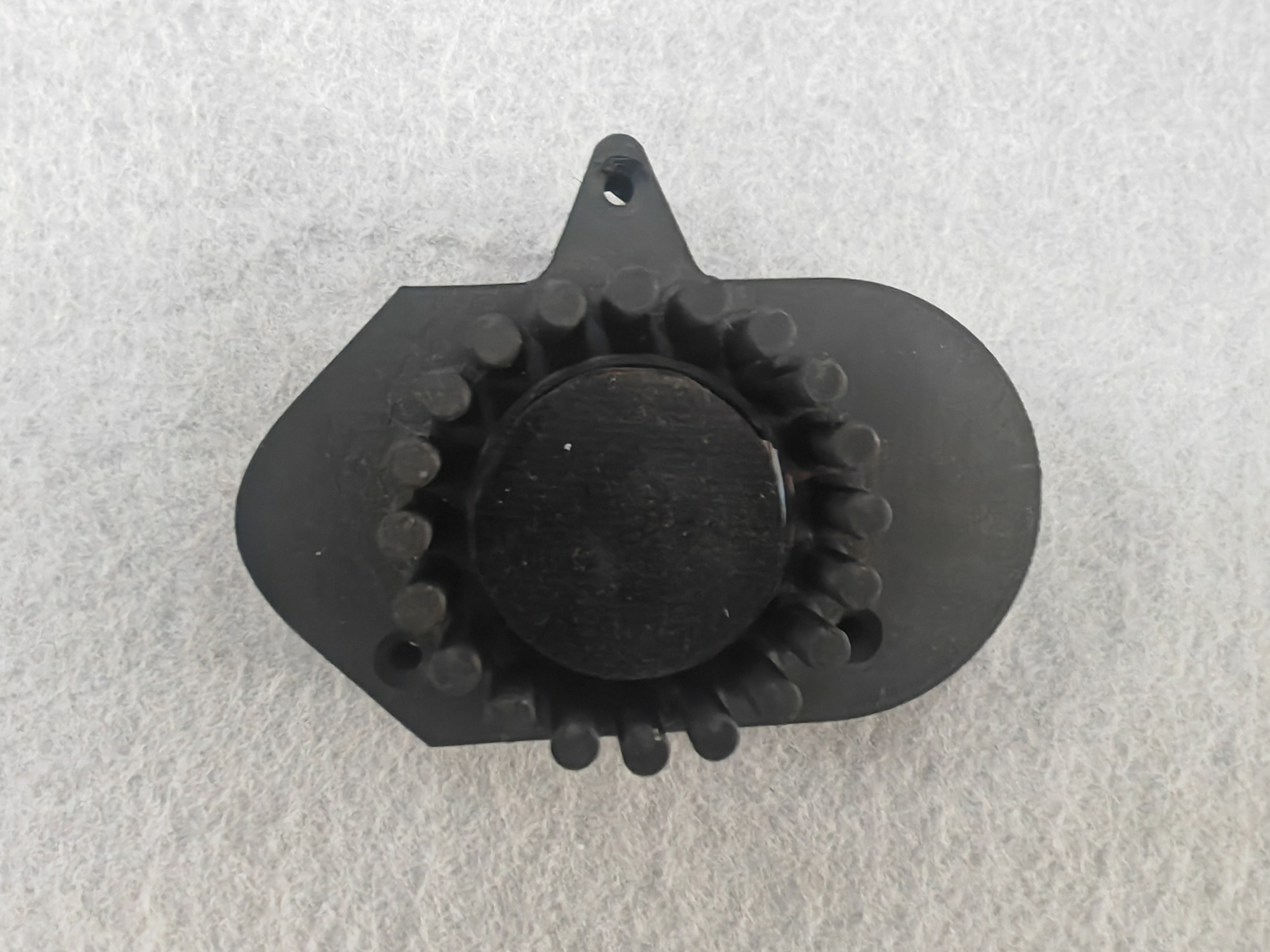
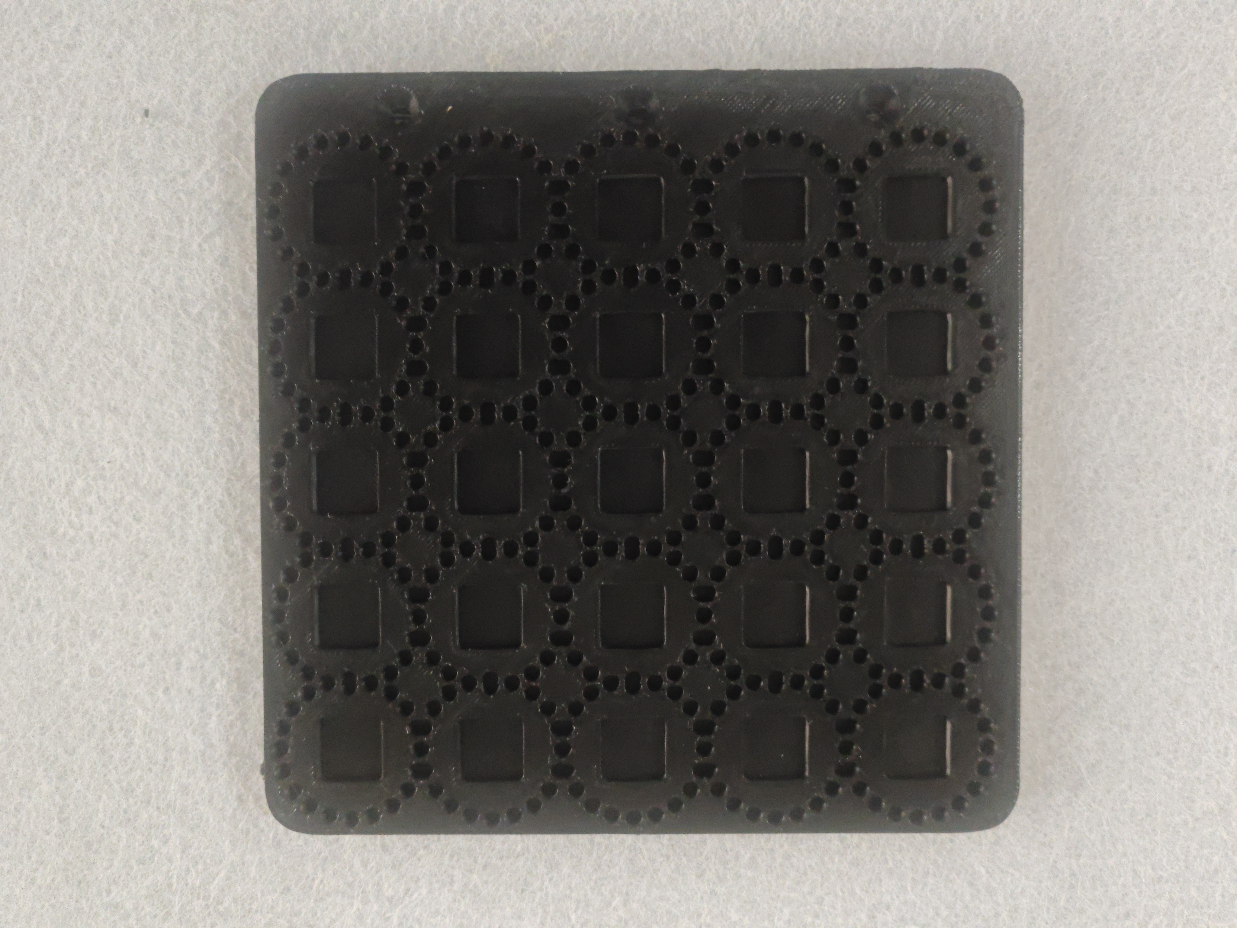
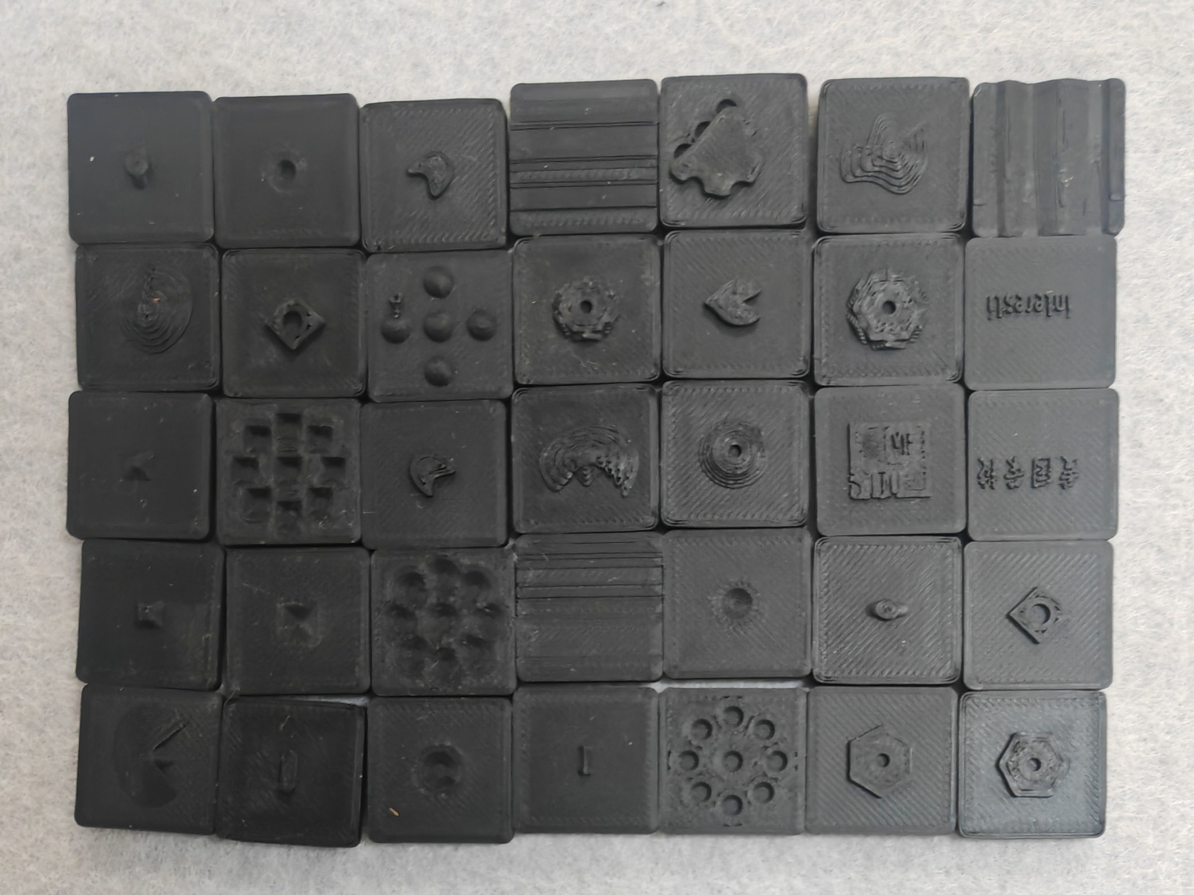
The same elastomer is first recorded without markers and then permanently marked and recorded again. A fixture with twenty indexed pin positions repeats object contact poses to reduce before/after misalignment. Fifty-four texture objects and twenty poses provide 1,080 paired examples. This avoids the indentation mismatch of synthetic dot overlays, while still requiring hardware fabrication and repeatable contacts.
Marker targets are pseudo labels: humans click marker centers and SAM 2 [53] provides masks, whose boundaries can be imperfect. Aligned crop/resize transformations change apparent marker scale, and marker-guided blur simulates defocus. These augmentations target some sensor variation, rather than sampling every possible elastomer, lighting, and marker design.
Equation 12
| (12) |
4 Experiments
Evaluation covers image restoration, marker localization, cross-sensor examples, loss ablations, and downstream force, surface, and fabric tasks.
4.1 Experimental Setup
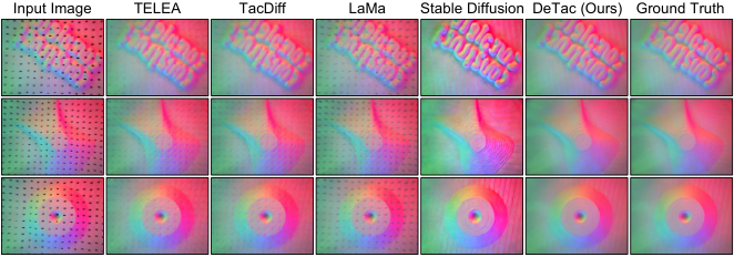
Training takes about fourteen hours on one RTX 4090 for three hundred epochs, with batch size two and separate learning rates of 10⁻⁵ and 10⁻⁴ for shading and markers. Five objects are held out entirely, and one pose from each remaining object is held out, leaving 931 training pairs and 149 test pairs. Comparisons include conventional inpainting, synthetic-data TacDiff/LaMa, a fine-tuned Stable Diffusion model, and deterministic regressors trained on the same real paired dataset. Metrics assess image fidelity/distribution and marker-centroid error; they should not be read as direct manipulation success.
| Method | Unseen pose | Unseen object | ||||||
|---|---|---|---|---|---|---|---|---|
| FID | KID | PSNR | SSIM | FID | KID | PSNR | SSIM | |
| TELEA [23] | 237.95 | 18.327 | 31.33 | 0.870 | 232.66 | 17.592 | 31.29 | 0.868 |
| TacDiff [21] | 158.94 | 11.447 | 31.52 | 0.866 | 155.63 | 10.654 | 31.40 | 0.863 |
| LaMa [54] | 358.16 | 37.535 | 29.09 | 0.804 | 360.27 | 37.117 | 29.16 | 0.803 |
| SD 1.5 [20] | 121.70 | 7.401 | 25.44 | 0.861 | 114.29 | 6.703 | 24.16 | 0.826 |
| U-Net | 108.35 | 7.489 | 38.56 | 0.950 | 111.28 | 7.750 | 39.03 | 0.942 |
| Pix2Pix | 112.53 | 7.472 | 38.53 | 0.951 | 109.66 | 7.065 | 38.98 | 0.948 |
| dual-head network | 104.27 | 6.923 | 37.99 | 0.949 | 105.18 | 6.794 | 38.37 | 0.947 |
| TacDiff (enlarged mask) | 172.01 | 11.898 | 30.93 | 0.852 | 180.96 | 12.384 | 30.84 | 0.847 |
| LaMa (enlarged mask) | 330.13 | 32.754 | 30.23 | 0.840 | 330.57 | 32.351 | 30.27 | 0.839 |
| DeTac (w/o ) | 25.78 | 0.733 | 34.64 | 0.946 | 22.59 | 0.698 | 35.05 | 0.945 |
| DeTac (w/o ) | 22.65 | 0.689 | 37.77 | 0.949 | 19.44 | 0.634 | 38.28 | 0.948 |
| DeTac (Full) | 20.44 | 0.683 | 39.45 | 0.953 | 17.06 | 0.573 | 39.07 | 0.950 |
| UVTac [17] | SAM 3.1 [55] | DeTac (w/o ) | DeTac (w/o ) | DeTac (Full) | |
|---|---|---|---|---|---|
| MCLE | 0.21 | 0.41 | 0.00839 | 0.00832 | 0.00762 |
4.2 Evaluation Results
DeTac achieves 39.45 dB on unseen poses and 39.07 dB on unseen objects, versus 31.52 and 31.40 for the reproduced TacDiff. The same-data U-Net is much closer at 38.56 and 39.03 dB, although its distributional metrics are substantially worse. Thus the headline gain over TacDiff includes a difference in training-data construction, while the paired-data regressors provide a closer comparison.
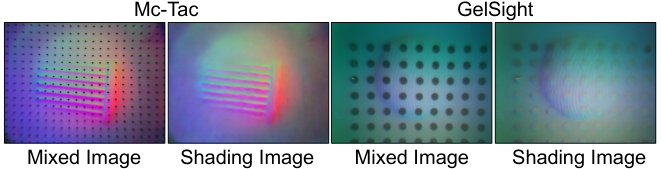
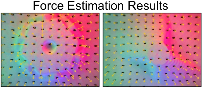
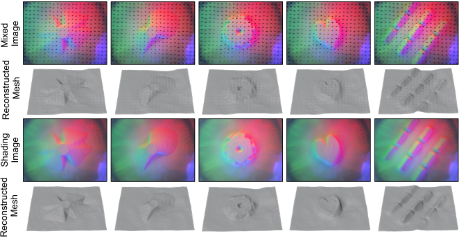
Marker-centroid error is 0.00762 mm versus 0.21 for UVTac and 0.41 for the listed SAM 3.1 baseline. The evaluation uses the paper’s pseudo-labeled marker supervision, not a separately described physical centroid metrology system. Cross-sensor transfer to altered illumination and another sensor is shown qualitatively in Figure 7; no aggregate cross-sensor success rate is reported.

4.3 Ablation Study
Removing the surrounding-region term lowers unseen-pose PSNR from 39.45 to 34.64 dB and unseen-object PSNR from 39.07 to 35.05. Removing the consistency term yields 37.77 and 38.28 dB. Both ablations also slightly increase centroid error. This supports the two auxiliary objectives under the studied dataset and training procedure; the largest shading effect comes from explicit supervision around markers.
4.4 Downstream Tasks
For force estimation, each representation receives its own trained downstream network, supervised by a six-axis force sensor transformed into the tactile frame. Table 3 reports mean force absolute error of 0.089 N with DeTac markers, versus 0.202 N for mixed images, 0.119 for UVTac, and 0.482 for SAM 3.1. This comparison combines the representation with a learned estimator, rather than evaluating a fixed universal force calibration.
Photometric stereo converts restored shading into surface meshes. Against aligned contact-region geometry from object models, Chamfer distance improves from 0.165 to 0.113 mm and root-mean-square error from 0.111 to 0.071 mm. Mesh alignment precedes scoring, so these numbers assess aligned reconstruction shape rather than unconstrained object pose accuracy.
5 Conclusion
Whole-image restoration and marker-aware joint supervision improve the tested tactile representations and downstream tasks. Limitations remain substantial: shading requires hundreds of sequential denoising steps, paired acquisition irreversibly modifies the elastomer and requires new hardware to scale, and the collection fixture does not support controlled shear. Cross-sensor examples do not establish general force transfer or fast closed-loop manipulation.
Acknowledgments
The authors acknowledge support from the National Natural Science Foundation of China, Shanghai science and technology programs, and the Beijing High Innovation Plan.
Appendix A Additional Implementation Details
The implementation appendix specifies both architectures, optimizer and diffusion settings, and contact-force consistency during paired capture.
A.1 Network Architecture Specifications
The shading U-Net concatenates mixed RGB and noisy-target RGB into six channels and outputs three-channel noise. Four downsampling stages use widths 64, 128, 256, and 256, with twenty-two residual blocks in total, Swish activations, and group normalization. The marker network uses three 3×3 convolutions with widths 3→32→64→1, ReLU between hidden layers, and sigmoid at output; training applies binary cross-entropy directly to logits.
A.2 Additional Training Details
Diffusion training uses one thousand timesteps. The surrounding-marker ring uses a two-pixel dilation radius. AdamW uses momentum coefficients 0.9 and 0.999, numerical epsilon 10⁻⁸, and weight decay 0.01. These complement the main-text loss weights of 0.5 for marker supervision and 0.05 for each auxiliary term.
A.3 Data Collection Details
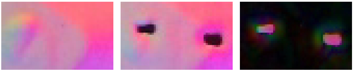
Twenty alignment pins constrain pose and pressing depth, while a 200 g weight standardizes loading. At identical depth, changing to 500 g produces a mean pixel difference of 3.072 on a 0–255 scale. This supports repeatable appearance under that specific loading comparison; it does not establish broad force or shear diversity. Figure A1 preserves the measured shading/mixed-image difference around embedded markers.
Appendix B Paired Dataset
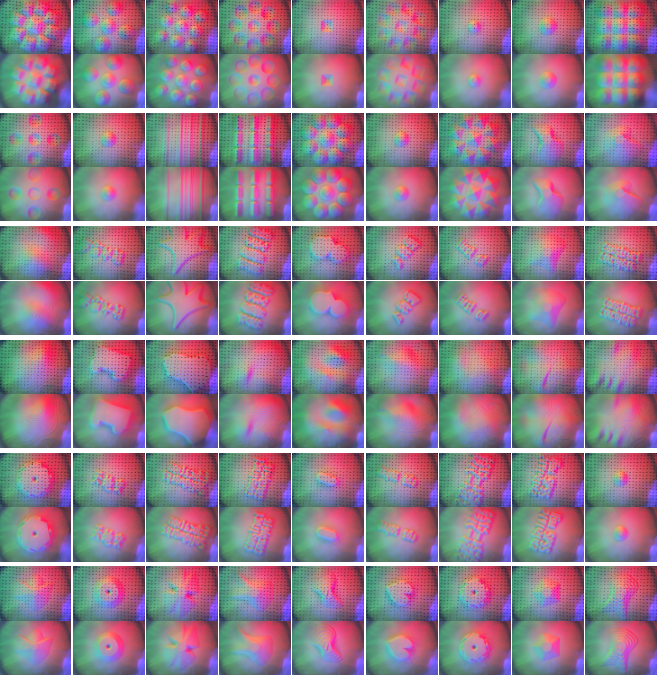
Figure A2 retains all fifty-four paired examples, one for each texture unit. Alternating mixture and marker-free rows expose the available texture diversity and the spatially matched restoration targets.
Appendix C Additional Experiments
A ResNet texture classifier is trained on markerless tactile data, then reused with a largely aligned marker-based sensor on a RealMan arm. Across thirty trials for each of three fabrics, replacing raw mixed images with DeTac shading raises overall classification success from 50.0% to 84.4%; per-fabric scores rise from 16.7/43.3/90.0% to 83.3/73.3/96.7%. This demonstrates compatibility with a fixed downstream tactile classifier on three fabrics. The mounted external camera is unused, and the experiment does not measure broader fabric categories or dexterous manipulation.
| Input Type | Success Rate | Overall | ||
| Fabric A | Fabric B | Fabric C | ||
| Raw mixed image | 16.7% | 43.3% | 90.0% | 50.0% |
| Our marker-removed shading image | 83.3% | 73.3% | 96.7% | 84.4% |