Overview
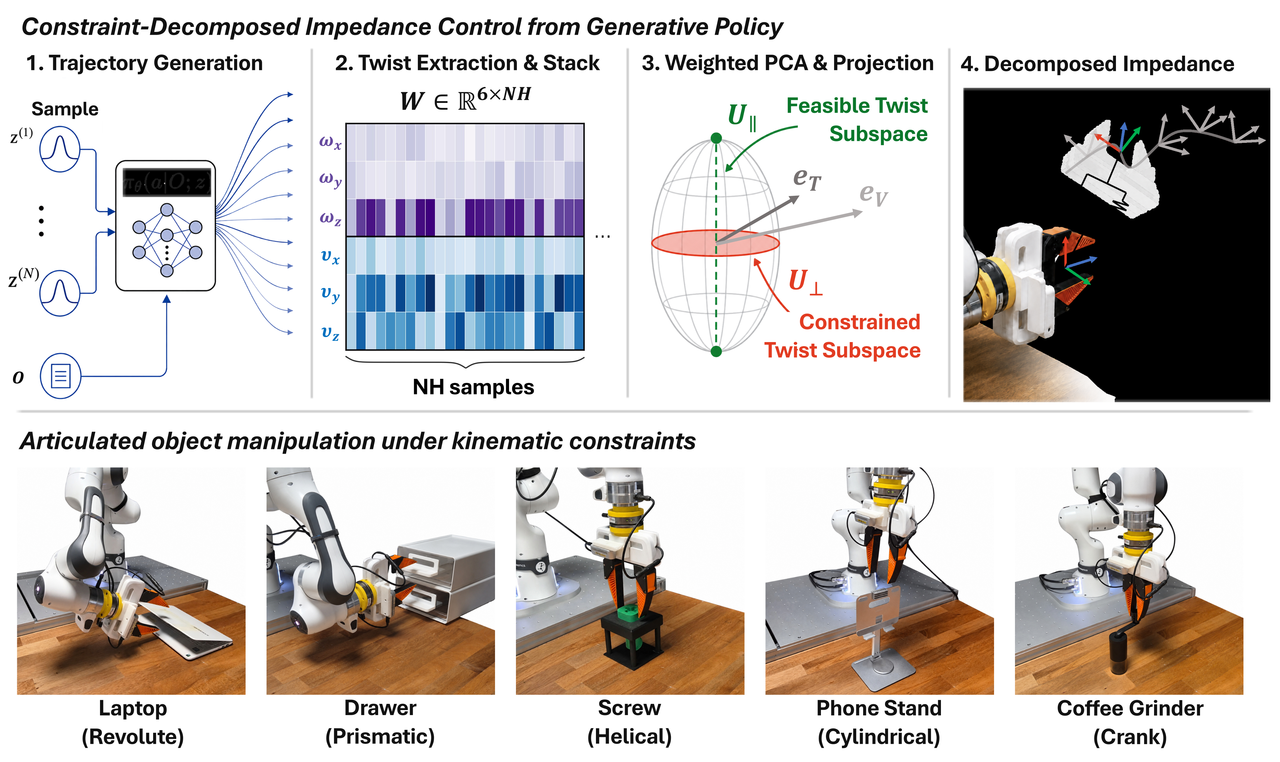
Read this as a method for shaping impedance after a successful grasp. It estimates motion directions from a generative policy and preserves compliance in their complement. All five figures, 14 numbered tables, 56 numbered equations and the complete algorithm remain; the extensive appendices define the controller’s local theoretical scope and experimental qualifications.
At a glance
Sample multiple end-effector trajectories at the same observation, convert them to body twists and estimate their dominant linear subspace with weighted, uncentered PCA. Fixed impedance gains track that subspace stiffly and soften its complement. For many single-joint mechanisms the feasible subspace is configuration-independent; for other mechanisms the method instead estimates a larger fixed envelope that can contain instantaneously infeasible directions. Simulation and physical tests usually reduce measured complementary loads, but the real crank’s force impulse increases 14%. The passivity result applies only to a local, frozen-inertia error model with fixed gains; it is not a general physical contact-safety guarantee.
1 Introduction
Small policy trajectory errors can create large forces when a rigidly grasped object cannot move in the commanded direction. Uniformly lowering stiffness also weakens useful motion. The proposed solution estimates the articulation’s directional structure from diverse policy samples and keeps high gains along supported motions. No separate perception model, physical probing or known screw axes enter the estimator. Its central assumption is that policy outputs collectively cover the relevant feasible directions. Gains are estimated once at grasp closure and held fixed during articulation, avoiding continuous geometry estimation at the cost of limited adaptation.
2 Related Work
The method differs from explicit articulation estimation and from rules that directly map positional variance or measured force to stiffness. Its geometry is the span of body twists generated by the policy.
Explicit articulation estimation.
Vision, interaction and demonstration methods can estimate joint axes or articulation models, but their results must be transformed into the grasp/controller frame. Here sampled end-effector trajectories already reflect the current grasp. Avoiding a separate estimator does not remove the need for informative demonstrations or correct body-frame conventions.
Variance-based impedance and direction-wise control.
Earlier variance-based control makes low positional variance stiff. This work uses twist variation differently: little motion in a direction suggests a constraint, so that direction becomes compliant. Subspace-wise hybrid control supplies the split as prior knowledge, while force-directed compliance uses a measured-force rule. The proposed split instead comes from policy-implied articulation geometry.
3 Preliminaries
Operational-space dynamics explain how pose/twist errors become commanded wrenches. Articulated-object kinematics explain which body twists belong to a local feasible subspace and when a fixed global subspace can represent them.
3.1 Operational-Space Impedance Control
The virtual mass–damper–spring relation links pose/twist errors to external wrench. Matching virtual inertia to operational-space robot inertia permits model-based acceleration/Coriolis/gravity feedforward plus stiffness/damping feedback, mapped to joint torques by the Jacobian transpose. High gains enforce tracking; low gains permit displacement under contact. The method changes directional gains, retaining the nominal operational-space implementation and its modeling assumptions.
Equations 1–2
| (1) |
| (2) |
3.2 Kinematics of Articulated Objects
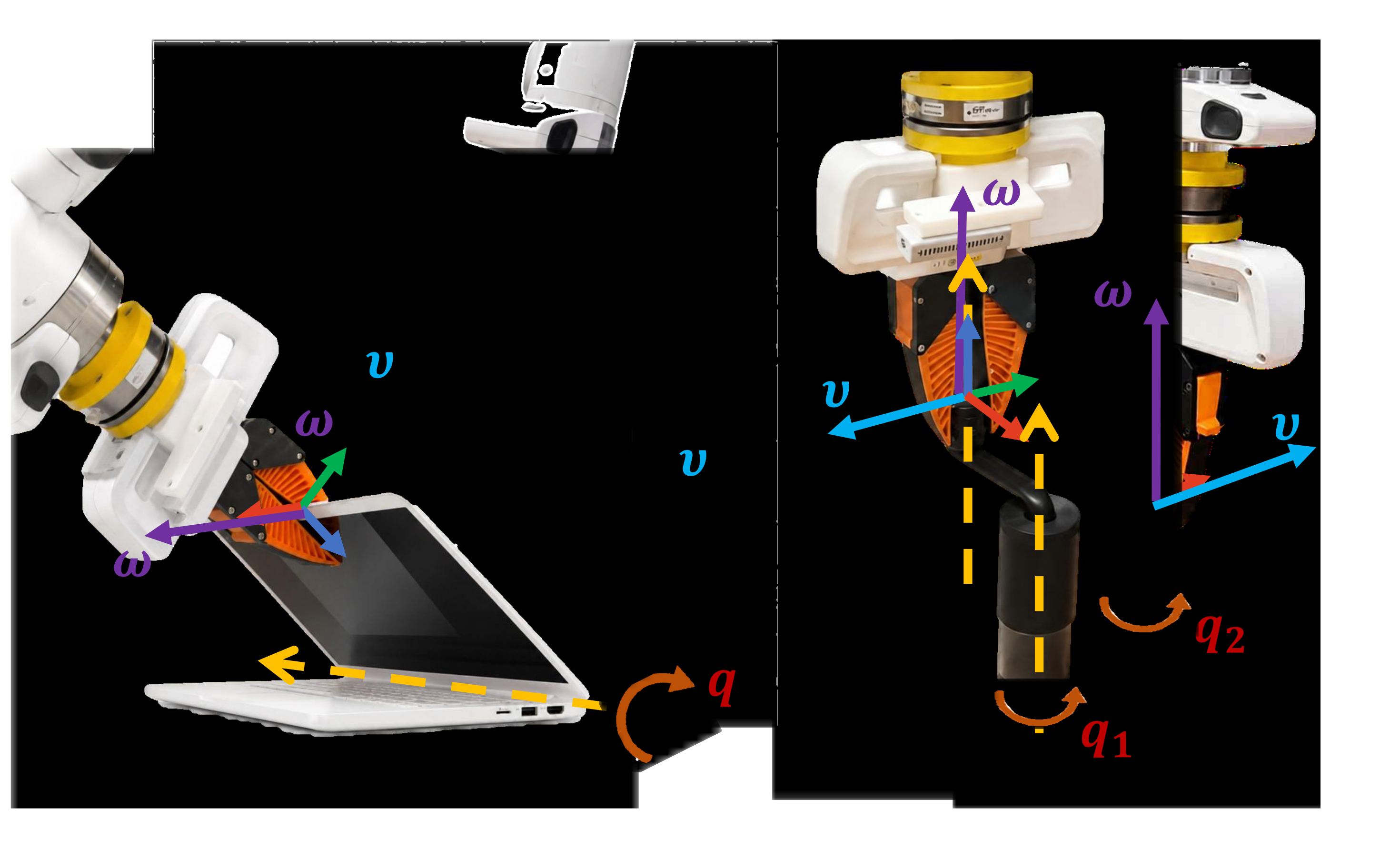
Model a fixed-base open chain with a rigidly grasped distal link. The range of its body Jacobian is the local feasible twist subspace. A laptop hinge has a fixed one-dimensional body-twist span; a two-joint coffee-grinder crank changes its local span with configuration. Define the global envelope as the smallest linear subspace containing all local spans. Membership is equivalent to feasibility only when the local span is constant; otherwise membership is necessary but insufficient. Singular configurations and grasp-frame transformations remain relevant.
Equation 3
| (3) |
Equation 4
| (4) |
4 Method
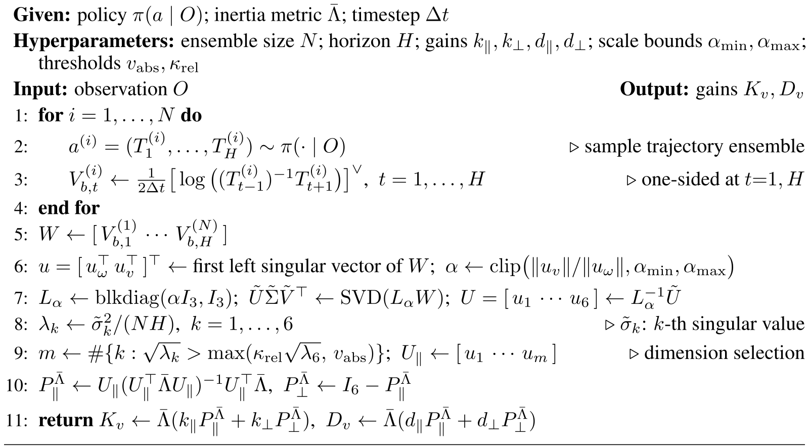
Given a generative manipulation policy, estimate a body-twist envelope from its outputs and convert that estimate into inertia-weighted gains. No retraining or supplied articulation parameters are required at deployment. Algorithm 1 preserves the exact sampling, finite-difference, rank-selection and gain computations.
4.1 Constraint Estimation from a Trajectory Ensemble
Each action is an H-step desired end-effector pose trajectory. At one visual/proprioceptive observation, sample an ensemble and infer the origin-passing subspace spanned by the resulting body motions.
Body twist extraction.
Finite differences on each SE(3) trajectory produce body twists, stacked into a 6×NH matrix. Multiple trajectories can suppress individual off-constraint errors and expose independent motions missing from a single rollout. This relies on diversity representing valid articulation alternatives rather than arbitrary policy noise.
Weighted PCA in twist space.
Choose a positive-definite twist metric G, factor it as LᵀL and apply SVD to LW; transform left singular vectors back by L⁻¹. The eigenvalues λk=σk²/(NH) are squared RMS speeds in the scaled metric. Keep leading directions whose square-root speeds exceed both an absolute floor and κrel times the least-excited square-root speed. The absolute test targets policy/sampler residual motion; the relative test addresses spectrum-wide grasp-chain deviations. Both are calibrated hyperparameters, not automatically known noise bounds.
Equations 5–7
| (5) |
| (6) |
| (7) |
Choice of the inner product.
Use G=diag(α²I, I), converting angular velocity into a linear-velocity scale. Estimate α from the translation/rotation norm ratio of the leading unweighted singular vector and clip it to a fixed range. This data-derived length sets PCA geometry; it is not the separate nominal-inertia length used to construct controller gains.
4.2 Impedance Gain Decomposition
A constant positive-definite block-isotropic inertia metric defines the feasible/complement projectors. The full Gram inverse is necessary because the PCA basis is orthonormal in G, not necessarily in this control metric. Body-frame double-geodesic pose error and adjoint-transported twist error feed inertia-weighted stiffness/damping maps. With fixed projectors and nonnegative gains, those maps are symmetric positive semidefinite; positive modal gains make them definite. The associated quadratic energy argument is local and first-order, with the precise limits given in AppendixF.
Equations 8–10
| (8) |
| (9) |
| (10) |
5 Experiments
Experiments test both estimation quality and contact loads under matched policies. Simulation includes an analytic-subspace oracle; hardware compares estimated decomposition against isotropic impedance.
Evaluation metrics.
Force and moment are projected separately onto complements of the analytic reference’s linear/angular spans. Impulse integrates magnitude; the reported “peak” is the 95th percentile, not the maximum. For configuration-dependent objects the reference is the fixed envelope, so these diagnostics omit local constraints inside it. Subspace error is a largest principal angle; simulation success counts completion of a common articulation range. AppendixH fixes the scoring metric and trial inclusion rules.
Compared controllers.
Iso uses equal normalized gains in all directions. Ours keeps the same feasible gains and reduces complementary stiffness; Oracle applies the same rule with an analytic grasp-conditioned subspace. Every comparison shares the same Diffusion Policy checkpoint. This isolates the chosen gain split within the experiment rather than comparing different learned policies.
5.1 Simulation Experiments
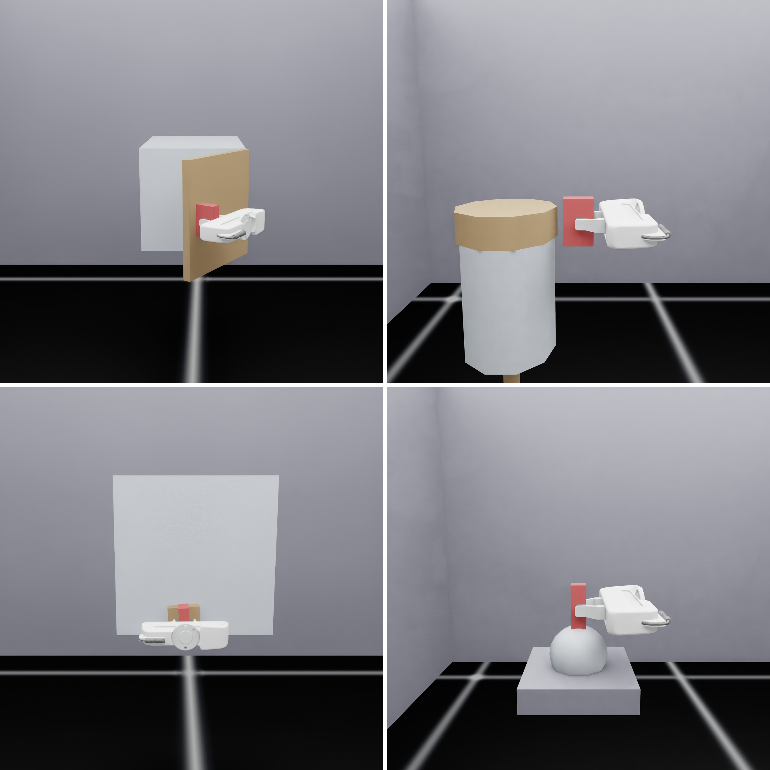
Four simulated mechanisms test one-, two- and three-dimensional motion spans, including a locally two-dimensional universal joint whose fixed envelope has dimension three.
Setup.
Isaac Sim uses a flying gripper on revolute, cylindrical, planar and universal joints. The policy predicts 24 poses at 0.1-second intervals; impedance runs 150 Hz. At grasp closure, sample 128 trajectories with ten DDIM steps, use 5 mm/s and relative threshold 4, and reduce complement stiffness to 0.1 of the feasible value. Evaluate 100 initial configurations per controller/object. Oracle supplies only the gain subspace, not a different tracking policy.
Results.
Force impulse falls to 0.13–0.37 of Iso and 95th-percentile force to 0.18–0.46, recovering at least 90% of the Oracle reduction in these metrics. Mean subspace errors are 1.64–4.36°. Success remains approximately 97–100%, with the complete counts preserved in Table 1. Wrench comparisons use the shared-success episodes, whereas success rates count every attempt. Moment components are small and the universal-joint angular complement is structurally empty. Multi-task results show similar force reductions.
| Task | SR (%) | SE (°) | ICF (Ns) | PCF (N) | ICM (Nms) | PCM (Nm) |
|---|---|---|---|---|---|---|
| Revolute | 099 / 099 / 099 | 1.64 | 7.18 / 2.62 / 2.13 | 3.38 / 1.56 / 1.48 | .29 / .22 / .22 | .19 / .18 / .17 |
| Cylindrical | 099 / 100 / 100 | 1.73 | 5.31 / 0.83 / 0.53 | 1.96 / 0.36 / 0.31 | .32 / .22 / .21 | .16 / .14 / .14 |
| Planar | 099 / 099 / 099 | 2.78 | 15.3 / 1.93 / 2.20 | 4.03 / 1.18 / 1.16 | .74 / .48 / .34 | .29 / .23 / .21 |
| Universal | 100 / 100 / 100 | 4.36 | 2.18 / 0.46 / 0.34 | 1.25 / 0.23 / 0.19 | – / – / – | – / – / – |
5.2 Real-World Experiments
Five physical objects include revolute, prismatic, helical, cylindrical and parallel-axis crank mechanisms. The crank tests the limitation of a fixed envelope for configuration-dependent motion.
Setup.
An FR3 runs impedance at 1 kHz and the same 24-step/0.1-second policy horizon. Estimate from 32 trajectories with 100 DDPM steps, absolute threshold 3 mm/s and relative threshold 10, except 4 for the crank; complement stiffness ratio remains 0.1. Each object has ten trials/controller from fixed object/base configurations. Gains and collision thresholds are tuned so both controllers complete all trials, enabling matched-progress wrench comparisons. This protocol does not establish a hardware success advantage or robustness over randomized initial poses.
Results.
Mean object-wise force impulse/peak ratios are 0.72/0.70; moment impulse/peak ratios are 0.69/0.56 with prismatic excluded. All four configuration-independent objects improve across reported loads. Subspace error is 13.01° for revolute and 2.89–5.76° for the others. The crank reduces peak force and moments but increases force impulse to 1.14×Iso: its envelope permits some locally infeasible directions to remain stiff. Table 2 preserves this exception.
| Task | SE (°) | ICF (Ns) | PCF (N) | ICM (Nms) | PCM (Nm) |
|---|---|---|---|---|---|
| Revolute | 13.01 | 46.6 / 25.2 (0.54) | 8.54 / 3.62 (0.42) | 5.00 / 3.34 (0.67) | 0.93 / 0.37 (0.40) |
| Prismatic | 04.74 | 12.3 / 8.79 (0.72) | 4.63 / 3.51 (0.76) | 1.84 / 1.46 (0.80)† | 0.61 / 0.55 (0.90)† |
| Helical | 02.89 | 6.96 / 6.50 (0.93) | 4.56 / 4.40 (0.96) | 1.82 / 0.60 (0.33) | 1.08 / 0.45 (0.41) |
| Cylindrical | 05.76 | 8.35 / 4.42 (0.53) | 3.37 / 2.20 (0.65) | 1.09 / 0.82 (0.75) | 0.45 / 0.37 (0.81) |
| Crank | 05.70 | 20.8 / 23.6 (1.14) | 4.62 / 4.28 (0.93) | 4.99 / 4.15 (0.83) | 1.12 / 0.82 (0.74) |
5.3 Analysis of Constraint Estimation
Post-hoc subset and perturbation studies separate ensemble count, sample diversity and noise effects. Many of these analyses hold the subspace dimension fixed, unlike deployment’s threshold-selected dimension.
Ensemble size and runtime.
With true dimension fixed, pooled 95th-percentile error falls from 78.9° at one sample to 23.1/8.59/7.23° at 2/4/8, reaching 6.61° at 128. Correct dimension on every trial requires at least 64 samples under one threshold setting. Batched 128-sample estimation and gain construction takes 70.1 ms median and 76.5 ms maximum on an RTX 5070 Ti; this one-time simulation sampler timing uses ten DDIM steps and is not the 100-step hardware sampler latency.
Sample diversity.
At equal subset size, high mean pairwise dynamic-time-warping diversity yields smaller errors than low diversity, especially at 2–8 samples. Mean per-object median error at k=2 is 5.91° versus 19.7°, approaching 2.34° for the full ensemble. By 32–64 samples the difference becomes small. Increasing N mitigates finite sampling gaps, but cannot reveal a feasible direction absent from the demonstrations or learned policy.
Robustness to noise.
A policy trained on noisy demonstrations attenuates some perturbations compared with adding the same noise directly to sampled trajectories. Five-degree orientation corruption still produces about 10.6° median subspace error. Tested image noise/blur/shifts barely change the clean 2.10° result; reducing denoising from 100 to 4 steps also changes little. The appendix’s two-step case collapses to 87.38°, so robustness does not extend to arbitrarily crude sampling.
6 Conclusion
Policy ensembles can identify useful motion directions for fixed impedance shaping, reducing complementary loads in the tested tasks without explicit online articulation estimation. The mechanism depends on body-twist coverage and appropriate metrics, not merely on producing more trajectories.
Limitations and future work.
Insufficient demonstration diversity or policy mode collapse can hide feasible directions at any ensemble size. A fixed envelope also leaves stiffness along some instantaneous constraints of configuration-dependent mechanisms. Local resampling and force/tactile refinement are future directions. The construction shapes gains under a nominal inertia metric; it does not fully decouple the real robot/object dynamics. Contact switches, large errors, online projector changes and true-inertia variation fall outside the provided passivity certificate.
Acknowledgments
The authors acknowledge Korean government research programs, Seoul National University institutes/programs, Hyundai Motor/Kia and Microsoft Research support. The listed grants and institutional acknowledgments remain attributable to the original paper.
Appendix A Operational-Space Dynamics and Block-Isotropic Inertia
AppendixA derives the feedforward/feedback wrench split, defines the fixed inertia surrogate and establishes body-coordinate tracking errors. It separates physical plant dynamics from the metrics used for estimation and gain design.
A.1 Commanded Wrench from the Virtual Impedance Model
Match virtual inertia to the body-frame operational inertia and equate the impedance target with the robot dynamics. Reference acceleration includes the derivative of adjoint transport. Under exact model matching, the resulting model-based acceleration/Coriolis/gravity terms plus spring/damper feedback recover the target relation. Contact wrench cancels from the command derivation, so measured force/torque is used for monitoring/evaluation, not controller feedback. Approximate models leave residual dynamics.
Equations 11–16
| (11) |
| (12) |
| (13) |
| (14) |
| (15) |
| (16) |
A.2 Block-Isotropic and Normalized Inertia
A configuration-dependent inertia could normalize dynamics but would make the directional metric vary online. Instead, use constant rotational/translational scalar blocks. This fixed gain metric differs from both the feedforward model inertia and the data-scaling PCA metric G. Its geometric role is to connect twist splitting and wrench generation; it does not eliminate physical angular/linear coupling.
Equations 17–20
| (17) |
| (18) |
| (19) |
| (20) |
Computing Λ ¯ .
Take trace averages of the rotational and translational diagonal inertia blocks at the control origin, discarding anisotropy and cross-coupling in the metric only. Simulation uses flying-gripper inertia; hardware uses FR3 operational inertia at a nominal payload-bearing pose. The actual plant still contains the omitted coupling. Table 6 gives platform-specific snapshots.
Equation 21
| (21) |
Scale normalization.
Multiplying the inertia metric by a positive scalar leaves its projectors unchanged and rescales wrench gains. Only the square-root inertia/mass length ratio changes projector geometry. Experiments normalize mass to 1 kg and absorb scale into scalar modal gains. These are not universal physical stiffness constants.
A.3 Body-Frame Tracking Error Definitions
Pose error combines the principal SO(3) logarithm with translation resolved in the current body frame, rather than the full SE(3) logarithm. Desired twist is adjoint-transported before subtracting current twist. The reference-minus-current sign produces restoring feedback. Near zero pose error, the pose-error derivative equals twist error to first order; finite errors require the exact chart relation derived later.
Equation 22
| (22) |
Appendix B Configuration Invariance from Lie Subalgebra
A sufficient configuration-invariance condition is that the span of home body screws form a Lie subalgebra. Each Jacobian column is an adjoint-transported home screw; the iterated-bracket expansion keeps it within a bracket-closed span. Equality with the local feasible subspace additionally requires full rank on the configuration range. At singularities only inclusion is guaranteed. Table 3 verifies common joint primitives; these analytic models are reference calculations, not estimator inputs.
Equations 23–24
| (23) |
| (24) |
| Primitive | DoF | Generators | Structure |
|---|---|---|---|
| Revolute (R) | Abelian | ||
| Prismatic (P) | Abelian (any dim) | ||
| Helical (H) | Abelian | ||
| Cylindrical (C) | Abelian | ||
| Spherical (S) | |||
| Planar (E) |
Spherical (S), worked.
For three rotations about a common point, the bracket of two generators yields the third; the span is isomorphic to so(3). Planar motion closes similarly as se(2), and shifting the origin changes the basis within the span. One-dimensional screws and the coaxial cylindrical pair commute. Mechanisms lacking this closure can have configuration-dependent body spans.
Equation 25
| (25) |
Appendix C Configuration Dependence and the Global Envelope
Three two-revolute-joint examples show how local dimension two can generate a larger fixed envelope. A distal-axis frame simplifies the screws; a different rigid grasp frame applies one adjoint to all of them. Claims assume nondegenerate axes/offsets and a nonempty interval of distal angles.
U-joint (worked example).
For intersecting perpendicular axes, the rotating proximal screw sweeps two angular directions; the constant distal screw supplies the third. The universal-joint envelope is all three-dimensional rotation, although only two directions are instantaneously feasible.
Equation 26
| (26) |
Parallel-offset crank (worked example).
For parallel offset axes, subtracting the distal screw leaves translation sweeping the plane. The crank envelope combines z-rotation with x/y translation, dimension three. The off-axis orthogonal door/lever example has envelope dimension four and is a theoretical example rather than an experimental object.
Equations 27–28
| (27) |
| (28) |
| Mechanism | Excitation for full | ||||
|---|---|---|---|---|---|
| U-joint (intersecting 2R) | excited, phases | ||||
| Parallel-offset crank (parallel 2R) | phases ( redundant) | ||||
| Door hinge lever (off-axis orthogonal 2R) | excited, phases |
Excitation.
A continuous angle sweep spans the sine/cosine-dependent screw components; a finite ensemble needs enough distinct phases and independent joint-velocity excitation to attain the envelope rank. A narrow range or nearly one-dimensional velocity pattern can underrepresent it even when the mechanism has more freedom.
Feasibility versus envelope membership.
The envelope is an outer bound: it contains every feasible twist but may also contain motions impossible at the current configuration. For the crank, both planar translations belong to the envelope while only one is feasible locally. Treating the whole envelope as stiff therefore leaves residual constraint loads, explaining an important experimental limitation.
Appendix D Trajectory-Ensemble Subspace Estimation in the PCA Metric
Because the desired subspace passes through zero, the estimator uses an uncentered second moment. Choosing a twist metric and its characteristic length is necessary before comparing angular and linear motion magnitudes.
D.1 Why a PCA Metric Is Required
Ordinary Euclidean PCA implicitly equates incompatible angular/linear units. G defines the meaningful norm; transformed SVD yields G-orthonormal directions and squared RMS eigenvalues. Rank selection gates square-root eigenvalues against absolute and relative speeds. The floor remains meaningful when the least mode is tiny; the relative gate tracks broader grasp-chain residuals. Threshold success in these calibrated experiments is not a universal rank-identification theorem.
D.2 Meaning of the Characteristic Length α
The characteristic length converts angular velocity to an equivalent linear scale. Its leading-mode norm ratio is computed in control-frame SI coordinates and clipped; pure translation saturates the upper bound. α is a data-dependent convention, not an invariant object property or the separate inertia length.
Equations 33–34
| (33) |
| (34) |
D.3 Why the PCA Is Uncentered
Centering removes the outer product of the mean twist, potentially deleting the main task-progress direction. For nearly constant one-DoF motion, uncentered PCA recovers the signal while centered PCA emphasizes residual noise. Exact noiseless recovery requires excitation rank equal to the envelope dimension; noisy recovery further depends on the spectral gap.
Equation 35
| (35) |
Appendix E Inertia-Metric Projectors and Energy-Consistent Gains
The appendix verifies metric-projector algebra and derives gains as local quadratic energy/dissipation Hessians. These algebraic properties alone do not establish global contact stability.
E.1 Λ ¯ -Orthogonal Twist Projectors
For any full-rank estimated basis, its inertia-weighted Gram matrix is positive definite. The resulting projectors are idempotent, complementary and self-adjoint in that metric; they preserve their subspace, annihilate the complement and have zero cross quadratic terms. Inertia-weighted projectors are symmetric positive semidefinite. The Gram inverse is essential when the basis comes from another metric.
Equations 36–39
| (36) |
| (37) | ||||||
| (38) |
| (39) |
Dual (wrench) projector.
Wrench projection is the transpose dual of twist projection under the power pairing. A complementary projected wrench does no work on an exactly estimated feasible twist. With subspace estimation error, that ideal reciprocity no longer holds exactly.
E.2 Energy/Rayleigh-Based Gain Derivation
Assign separate quadratic elastic and Rayleigh costs to feasible and complementary errors. Projector identities reduce their Hessians to the proposed stiffness/damping maps. This is a conservative potential for the linearized pose-error dynamics; it is not a globally conservative SE(3) spring for arbitrary finite error.
Equations 40–41
| (40) |
| (41) |
E.3 Symmetry, PSD, and SPD
Nonnegative modal gains yield symmetric positive-semidefinite maps. Strictly positive gains on both complementary components make stiffness and damping positive definite by the metric Pythagorean identity. The experiments retain small positive complement gains, avoiding unregulated zero-gain error directions.
Equation 42
| (42) |
Appendix F Closed-Loop Error Dynamics and Local Passivity
The proof studies constant gains, first-order error kinematics and plant inertia frozen at an operating point. It establishes an error-coordinate dissipation inequality for that nominal model, with explicit residual terms explaining why broader claims do not follow.
F.1 Local Error Dynamics
First derive exact local pose-error kinematics within a single rotation-log chart, then linearize and freeze the compensated plant. The gain metric and actual frozen plant inertia remain distinct.
Local error chart.
Relative rotation and body translation errors yield an exact chart matrix using the inverse SO(3) left Jacobian and a translation cross-product block. That matrix becomes identity near zero error, giving the first-order relation. The derivation requires smooth references and a single-valued principal rotation logarithm, away from its cut locus.
Equations 43–44
| (43) |
| (44) |
Frozen nominal model.
Substitute modeled feedforward plus spring/damper feedback into the true body dynamics. Freeze the inertia at a positive-definite operating-point value and omit remaining inertia variation, higher-order geometry and model errors. The resulting constant-coefficient impedance equation is the plant used by the certificate, not the full nonlinear robot/object dynamics.
Equation 45
| (45) |
F.2 Storage Function and Local Passivity
Kinetic error energy plus quadratic elastic energy has derivative equal to negative damping dissipation plus the error-twist/contact-wrench supply. Positive stiffness and damping imply exponential stability of the unforced linear frozen model; semidefinite gains imply only the dissipation bound. The supply uses error velocity, so it is not automatically physical contact-port passivity under a moving reference.
Equations 46–49
| (46) |
| (47) |
| (48) |
| (49) |
Scope.
The inequality assumes modeled feedforward cancellation, fixed projectors, first-order pose kinematics and frozen plant inertia. Exact geometry adds a higher-order term without fixed sign; changing gains adds an energy-variation term; changing plant inertia and model error add further residual power. Large errors, contact switches or online projector updates can invalidate the bound. No global manipulation stability or exact inertial decoupling is proved.
Appendix G Gain Construction and Scaling
Scalar gains are chosen through natural-frequency/damping-ratio design targets, then multiplied by the normalized inertia metric. The formulas describe the gain convention, while numerical platform settings are separately reported.
G.1 Second-Order Gain Rule
Replacing the frozen plant inertia by the surrogate produces a normalized modal design equation. Match its stiffness to squared natural frequency and damping to twice damping ratio times natural frequency. This decoupled scalar design model is not a claim that the real coupled plant has the same modes or damping ratio.
Equations 50–52
| (50) |
| (51) |
| (52) |
G.2 Iso, Ours, and Oracle Gains
Iso, Ours and Oracle share the same feasible stiffness and damping targets. A single complement stiffness ratio r changes only the constrained side; r=1 recovers Iso.
Iso.
Equal gains collapse the projector split into block-isotropic inertia-weighted stiffness/damping. Iso therefore needs no subspace estimate and provides the reference load baseline.
Equation 53
| (53) |
Ours.
Ours sets complement stiffness to r times the reference and complement damping to √r times reference damping, preserving the normalized damping ratio. At r=0.1, damping is not reduced by the same 0.1 factor. Feasible gains remain identical to Iso.
Equation 54
| (54) |
Oracle.
Oracle uses the identical scalar rule and analytic grasp-conditioned reference subspace. In simulation its difference from Ours isolates subspace estimation within this setup, rather than a different compliance magnitude.
Appendix H Experimental Configuration
Implementation details specify estimator thresholds, inertia/gain values, policy training, demonstration coverage, sensing and trial scoring. These details are necessary to interpret both the load reductions and the theoretical assumptions.
H.1 Hyperparameters
Table 5 preserves common horizon, ensemble, sampling, characteristic-length clipping and threshold settings. Platform-specific gains are in Table 6.
| Group | Symbol | Value |
| Estimation | Ensemble size | (simulation); (real) |
| Trajectory horizon | ||
| Absolute threshold | mm/s (simulation); mm/s (real). | |
| Relative threshold | (simulation); for revolute, prismatic, helical, and cylindrical objects and for the crank (real). | |
| Sampler at grasp closure | DDIM, steps (simulation); DDPM, steps (real). | |
| Characteristic-length clip | ||
| Finite-difference timestep (s) | ||
| Control | Modal gains | Per-platform; see Table 6. |
| Reduction ratio | (Ours, Oracle); (Iso). |
Dimension-selection thresholds.
Calibrate the absolute gate from residual speed on known constraint-consistent training examples and the relative gate from intended grasp-chain compliance/clearance. The absolute gate alone selects correct dimension in all 398 successfully grasped simulation trials; the relative gate alone does so in all 50 hardware trials using the crank-specific value 4. These thresholds use prior calibration and an object-specific exception despite requiring no articulation model online.
Sensitivity to the characteristic length.
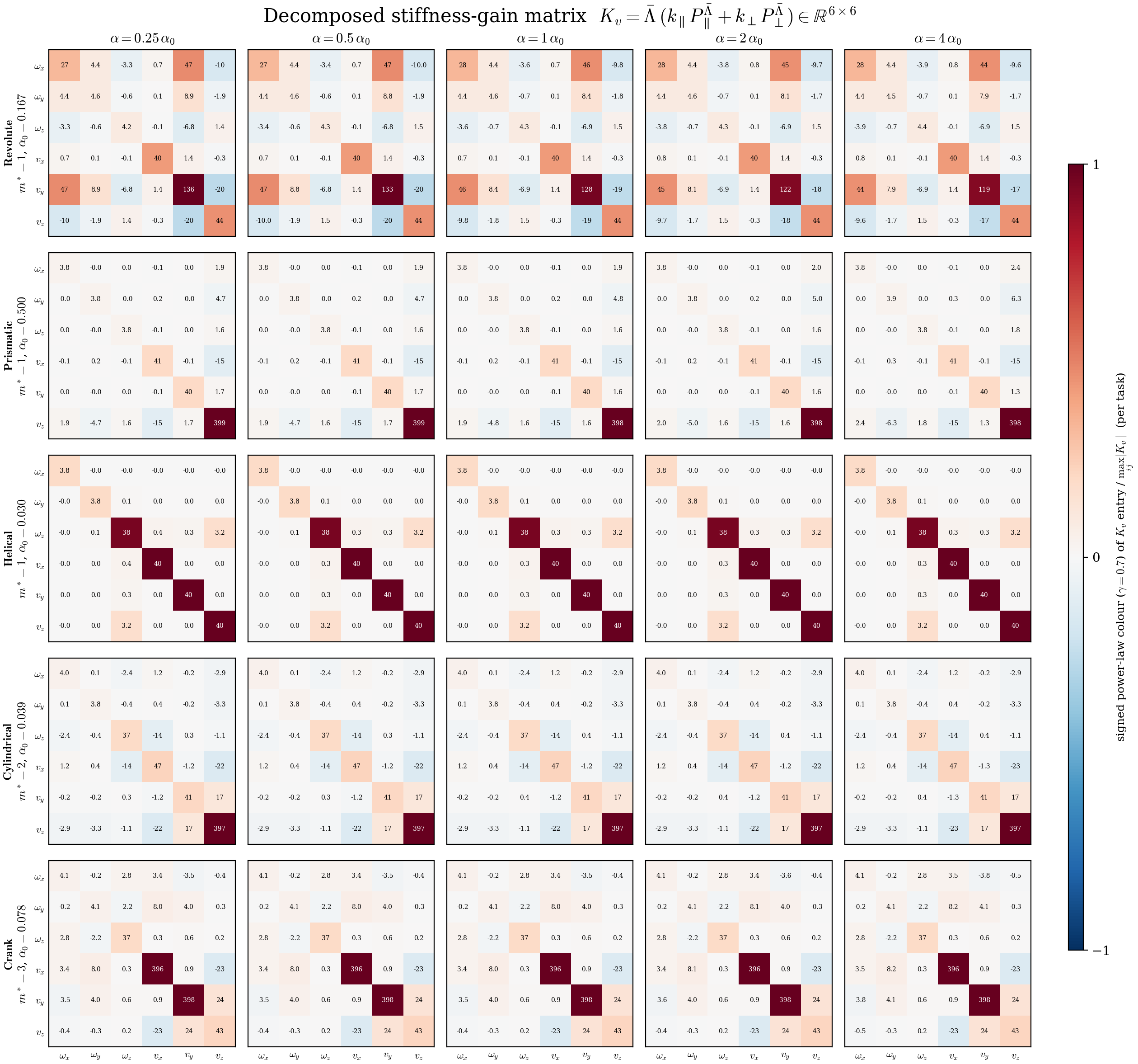
One representative real rollout per object varies α by factors 0.25, 0.5, 2, 4 at fixed dimension. The largest subspace change is 1.7° under the inertia metric. Figure 4 retains all 25 stiffness matrices: changing α rotates the estimated split but does not rescale the fixed modal gains. This small sample sensitivity study is not a full robustness guarantee.
H.2 Numerical Gain Values
Table 6 gives flying-gripper and FR3 inertia snapshots and gains. The mass-normalized convention uses 1 kg; the chosen damping ratio critically damps the surrogate design model, not a measured robot/object system. Ours/Oracle reduce complement stiffness by 0.1 while Iso uses 1.
| Platform | ||||||||||
|---|---|---|---|---|---|---|---|---|---|---|
| Flying gripper (sim) | ||||||||||
| FR3 (real) |
H.3 Implementation Details
All comparisons share policy interfaces and training checkpoints. Simulation and real control have different feedforward, rate and data details, preserved below.
Policy.
Object-specific Diffusion Policies train from scratch. A separate simulation policy trains equally on all four objects without a task identifier. Table 7 preserves the CNN/diffusion training recipe, relative pose-action interface and checkpoint-selection rules; diversity is inherited from the demonstrations rather than enforced by the controller.
| Setting | Value |
|---|---|
| Backbone | Diffusion Policy [21] |
| Observation history | step |
| Predicted / executed action horizon | / steps |
| Policy sampling period | s ( Hz) |
| Observation | wrist RGB, end-effector pose (position -D rotation), and gripper opening () |
| Action | Per-step relative pose chunk in the current EE frame: pose () and gripper command () |
| Visual encoder | ResNet-18 + spatial softmax |
| Denoising steps (train / infer) | / DDIM (simulation), DDPM (real) |
| Optimizer | AdamW, , weight decay |
| Learning rate | , cosine decay |
| Batch size | |
| Training length / checkpoint | Sim: steps/epoch; the first checkpoint (saved every epochs) after the validation-loss minimum, epoch /// for revolute/cylindrical/planar/universal; multi-task: epoch , the validation minimum. Real: steps/epoch, epochs; epoch- (k steps) |
Platforms.
Simulation uses a gravity-free flying gripper at 150 Hz with zero desired twist and feedforward, omitting Coriolis/reference-acceleration terms. Hardware uses torque-controlled FR3 with dense desired poses at 1 kHz and aligned evaluation recording at 100 Hz. Thus the full nominal dynamic cancellation proof is not a claim that every experimental implementation exactly realizes those assumptions.
Simulation demonstration data.
Collect 400 scripted demonstrations per simulated object using analytic handle kinematics, withheld from the policy/estimator/controller at evaluation. Randomized object poses and independently timed smooth joint-coordinate profiles span synchronous through sequential multi-DoF motions. A fixed schedule would undermine the motion coverage needed for subspace recovery. Table 8 preserves placement ranges and grasp setup.
| Item | Value |
|---|---|
| Demonstrations | scripted rollouts per object |
| Object placement | Uniform , , m, yaw |
| Gripper start | Fixed at m before approach and grasp |
| Waypoint generation | Object progress mapped to handle poses by analytic forward kinematics, interpolated on |
Real-world demonstration data.
Leader–follower teleoperation supplies 20 demonstrations each for revolute/prismatic/helical and 32 each for cylindrical/crank. Train on the follower’s actual constrained end-effector poses, not leader commands. This makes observed actions approximately feasible despite imperfect commands and is central to the estimator’s validity. Data are recorded at 10 Hz.
Contact and force sensing.
Simulation contact wrenches and an ATI Axia 80 wrist sensor supply evaluation and safety monitoring. No wrench feedback enters the proposed estimator or impedance law. Both hardware controllers share tuned safety thresholds and a common articulation interval.
Evaluation metrics.
Project force and moment separately using linear/angular blocks of the analytic reference; these marginal diagnostics are not a full screw-coupled reciprocal-wrench norm. Load fractions λ measure complementary measured impulse, whereas feedback fractions β measure reference-parallel commanded feedback, excluding feedforward. Structural empty blocks produce predetermined fractions. Evaluate principal-angle error with a fixed geometry-derived length per object, not each estimator’s chosen α. Simulation success counts grasp/target failures, while wrench means use the common-success set. All ten physical trials are retained and compared over the same absolute articulation target.
Evaluation sampling.
Use 100 trials per simulated controller/object for both policy types and ten per physical pair, with the hardware epoch 150 checkpoint. Estimate gains once at completed grasp; simulation blends from isotropic gains over 50 control steps (about 0.33 s) before holding them fixed. The transient blend is not included in the fixed-gain passivity proof.
End-to-end real-rollout visualization.
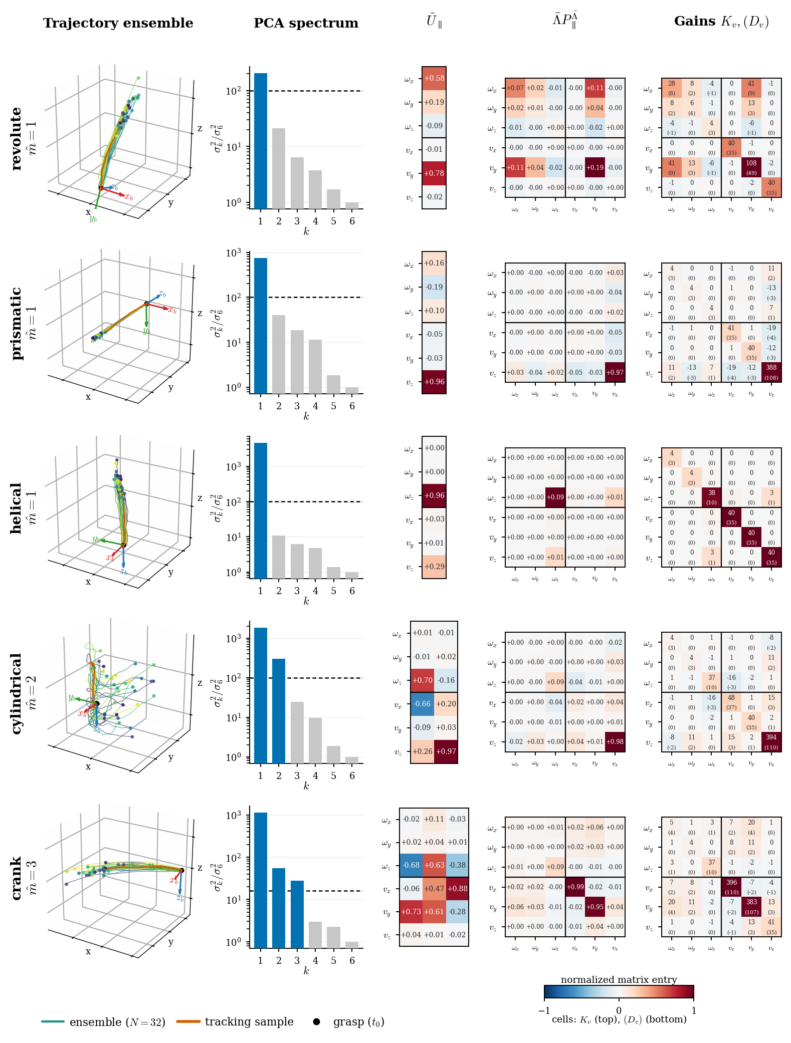
Figure 5 retains each real task’s 32-trajectory ensemble, singular spectrum/rank gate, weighted basis, inertia-projector matrix and final stiffness/damping entries. It demonstrates the full numerical pipeline rather than only final scalar load results.
Appendix I Simulation Experiments: Additional Results and Diagnostics
Table 9 reports force/moment fractions over matched three-controller successful episodes. Ours shifts feedback toward the reference-feasible block and generally lowers complementary measured load. The analytic reference and inclusion rules remain common across controllers.
| Task | |||||
|---|---|---|---|---|---|
| Single-task policies | |||||
| Revolute | 099 | .26 / .12 / .10 | .245 / .177 / .181 | .75 / .92 / .95 | .86 / .96 / .96 |
| Cylindrical | 099 | .15 / .03 / .02 | .122 / .086 / .084 | .85 / .98 / .98 | .94 / .98 / .98 |
| Planar | 099 | .68 / .21 / .24 | .114 / .077 / .057 | .32 / .81 / .78 | .90 / .95 / .98 |
| Universal | 100 | .31 / .14 / .11 | .000 / .000 / .000 | .69 / .87 / .91 | 1.00 / 1.00 / 1.00 |
| Multi-task policy | |||||
| Revolute | 099 | .27 / .13 / .11 | .242 / .197 / .190 | .74 / .92 / .94 | .86 / .96 / .95 |
| Cylindrical | 095 | .13 / .04 / .02 | .119 / .076 / .077 | .87 / .96 / .98 | .93 / .98 / .98 |
| Planar | 100 | .68 / .22 / .24 | .112 / .078 / .056 | .32 / .81 / .78 | .90 / .95 / .98 |
| Universal | 099 | .29 / .14 / .11 | .000 / .000 / .000 | .72 / .88 / .92 | 1.00 / 1.00 / 1.00 |
Multi-task policy.
The shared four-object policy preserves the main effect: force impulse becomes 0.14–0.37 of Iso, recovering at least 80% of the Oracle force improvement. Table 10 retains all success counts and complementary moment results.
| Task | SR (%) | SE (°) | ICF (Ns) | PCF (N) | ICM (Nms) | PCM (Nm) |
|---|---|---|---|---|---|---|
| Revolute | 099 / 099 / 099 | 1.71 | 7.75 / 2.87 / 2.55 | 3.55 / 1.76 / 1.81 | .31 / .26 / .26 | .21 / .22 / .22 |
| Cylindrical | 096 / 097 / 096 | 2.39 | 4.61 / 1.36 / 0.64 | 1.74 / 0.67 / 0.51 | .31 / .20 / .21 | .15 / .13 / .15 |
| Planar | 100 / 100 / 100 | 2.76 | 14.4 / 2.02 / 2.21 | 3.85 / 1.13 / 1.13 | .73 / .49 / .34 | .29 / .24 / .22 |
| Universal | 099 / 100 / 100 | 3.83 | 1.98 / 0.45 / 0.33 | 1.17 / 0.23 / 0.19 | – / – / – | – / – / – |
Ensemble size and runtime.
Table 11 shows errors decreasing sharply through four samples and more slowly afterward. Perfect dimension selection begins at 64 samples. The 70.1 ms runtime is the median of four per-object medians across 120 runs; 76.5 ms is the overall maximum, not a hardware control-loop period.
Sample diversity.
The diversity study selects extreme subsets among 4,012 candidate subsets of each ensemble. Benefits are largest up to 16 samples and nearly disappear at 32–64. This post-hoc selection study explains coverage; it is not the deployed collection algorithm.
Robustness to noise.
Table 13 separates action-noise training/direct injection, image corruption and denoising-count effects. Five-degree demonstration noise still produces 10.59° median error even if policy validation loss/success appear acceptable. Two DDIM steps yield 87.38° error, a clear failure outside the reported 4–100-step robustness range.
Appendix J Real-World Experiments: Additional Results and Diagnostics
Table 14 preserves every real auxiliary load/feedback fraction. Mean complementary fractions decline, but force fraction rises slightly for helical and more for crank; the crank nevertheless improves moment alignment substantially. Prismatic moment fractions are structural because it has no feasible rotational component. These diagnostics complement, rather than replace, the matched-progress force/moment magnitudes.
| Task | ||||
|---|---|---|---|---|
| Revolute | .766 / .672 (.88) | .734 / .522 (.71) | .738 / .843 (1.14) | .717 / .848 (1.18) |
| Prismatic | .362 / .321 (.89) | 1.000 / 1.000 (1.00) | .848 / .918 (1.08) | .000 / .000 (–) |
| Helical | .412 / .424 (1.03) | .724 / .569 (.79) | .187 / .332 (1.78) | .751 / .890 (1.18) |
| Cylindrical | .244 / .126 (.52) | .536 / .421 (.79) | .708 / .894 (1.26) | .572 / .680 (1.19) |
| Crank | .425 / .469 (1.10) | .926 / .850 (.92) | .841 / .892 (1.06) | .261 / .550 (2.11) |