Overview
The authors release code and a project website for their structured latent world model.
At a glance
Intuition: an ordinary learned predictor can repeatedly squeeze different states together until a long imagined trajectory loses motion information. LeHami replaces that predictor with a learned Hamiltonian and a volume-preserving leapfrog update. Its latent state has position-like and momentum-like halves, with the latter estimated from recent encoded frames. The construction prevents particular rollout-collapse mechanisms and supports changing the integration step. It does not guarantee accurate predictions, prevent encoder collapse or recover the true physical Hamiltonian. Experiments use conservative and driven simulated pendulums. LeHami improves several velocity-prediction and compute measures, while a baseline with a suitably asymmetric temporal encoder achieves higher goal-reaching success.
1 Introduction
The paper separates encoder collapse during learning from contraction caused by repeatedly applying a predictor. Training regularization can address the first without preventing the second. Hamiltonian structure constrains every deployed transition. Position and motion also require different evidence: one image may show where a pendulum is while leaving its direction of travel ambiguous.
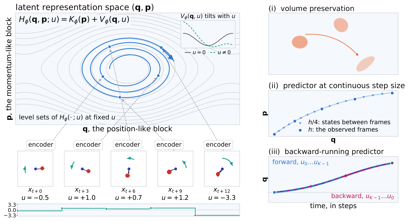
Contributions.
The contributions are a symplectic predictor, a fixed derivative channel, analysis of the collapse modes excluded by the update, and pendulum experiments on forecasting and planning. Architectural guarantees concern the latent map. Empirical physical readouts are needed to assess what the learned state actually contains.
2 LeHami: Symplectic Hamiltonian JEPA
Imagine a small cloud of starting states. A symplectic update can stretch and shear it but preserves its volume. With the stated smoothness and fixed-action-within-step conditions, leapfrog is invertible and cannot uniformly shrink every direction or merge distinct latent states. Volume preservation allows some directions to contract if others expand; it supplies no bound on prediction error or numerical stability at a large step size. The original formal statements are retained below.
Proposition 1 (Symplectic volume preservation and the rollout failure modes it removes).
Let be the leapfrog step of Eq. 4 for step size generated by a separable with held fixed within the step. Then is an exactly symplectic diffeomorphism of for every step size and every parameter ; it then preserves phase-space volume exactly at every horizon. Here is the integrator’s step, which equals the observation interval during training but need not at inference (Section 3.3). Consequently, three collapse modes are ruled out: uniform contraction, convergence to an asymptotically stable fixed point, and the merging of distinct states. They are stated and proved in Appendix C.1.
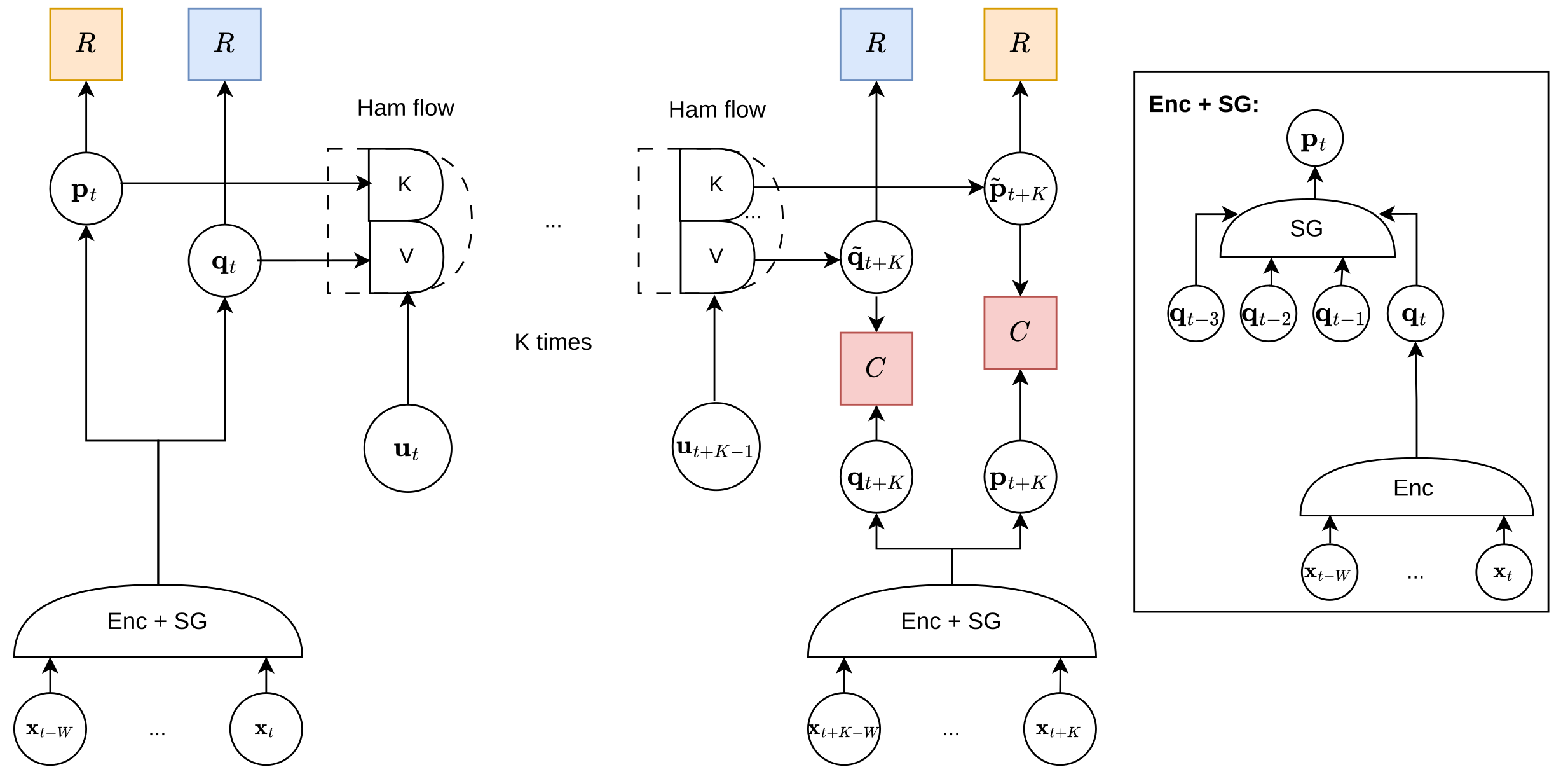
2.1 The architecture
The encoder outputs position-like features. A fixed Savitzky–Golay derivative of recent features initializes the momentum-like half. Two neural networks define a separable scalar Hamiltonian: one depends on momentum, the other on position and action. A kick–drift–kick update advances the pair, and multi-step prediction losses train it against encoded trajectories. SIGReg still shapes encoder features. After initialization, momentum evolves inside the predictor rather than being recomputed from future images.
Equations 1–5
| (1) | ||||
| (2) |
| (3) |
| (4) | ||||
| (5) |
2.2 Related work
Related models also impose mechanical structure, but differ in whether they reconstruct images, add dissipative dynamics, learn a separate control port or use a non-symplectic integrator. The same H-JEPA label appears in an independent Hamiltonian paper; it should not be confused with the hierarchical H-JEPA edition in this collection.
3 Empirical validation of LeHami
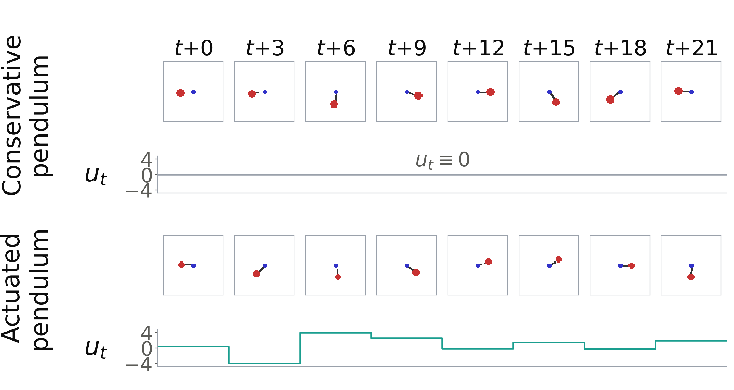
Two simulated pendulum systems test the model: an unforced system and one driven by recorded torques. Both preserve physical phase-space volume, matching the chosen structural prior. Rod lengths vary, and the driven system also varies mass. These are favorable mechanical testbeds rather than evidence for arbitrary dissipative environments.
3.1 Experimental setup
The main comparison shares training data, encoder family and learning setup with LeWM, changing the predictor and adding the derivative channel. Frozen probes read angle and angular velocity from features. Using a probe fitted after one predictor step gives LeWM access to temporal context; anchor-only comparisons otherwise favor a state with an explicit history-derived motion channel. Planning uses CEM with feedback replanning.
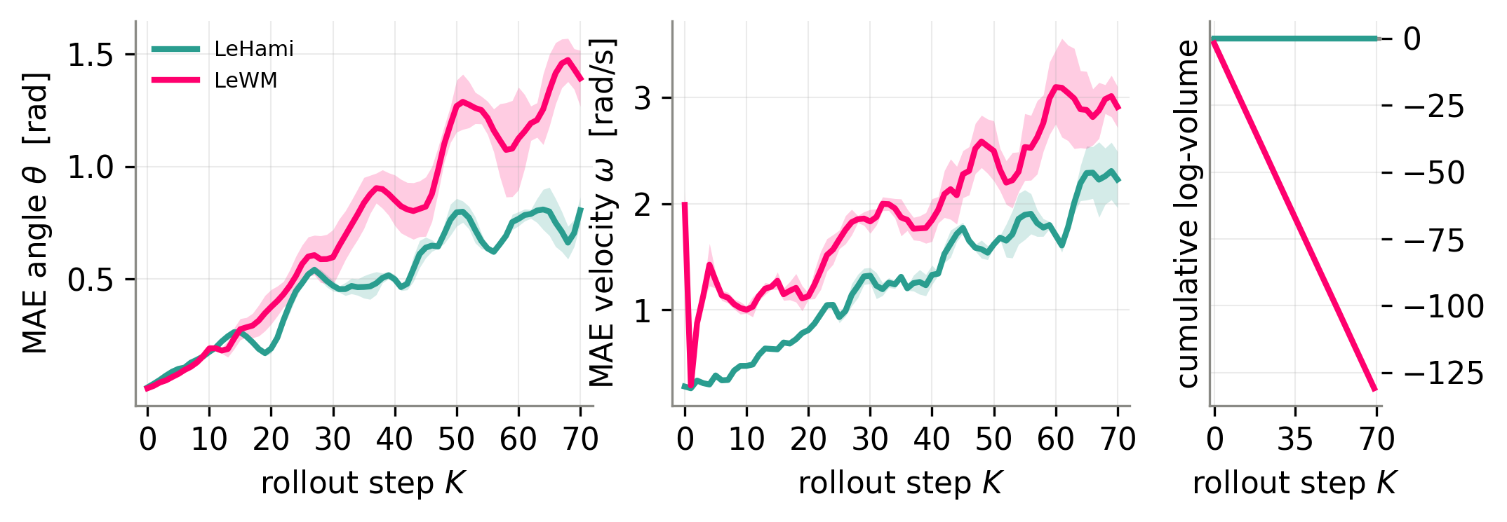
3.2 Evaluating Complete Phase-Space Physics Capture
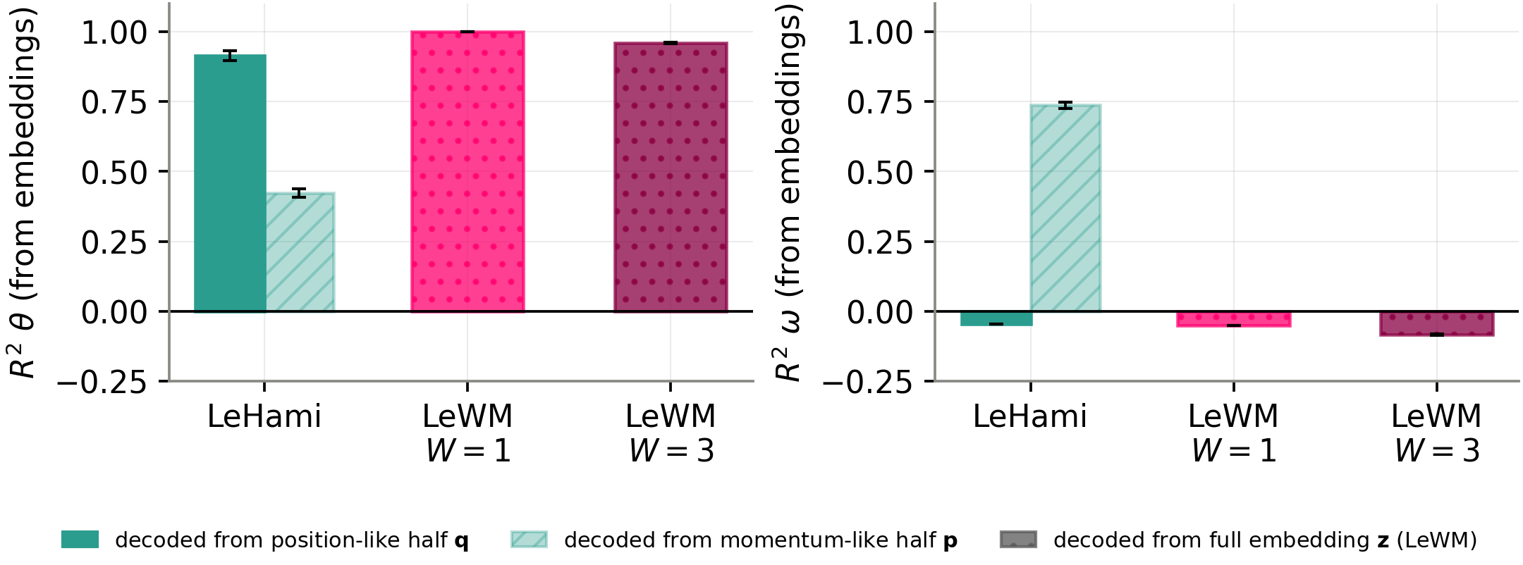
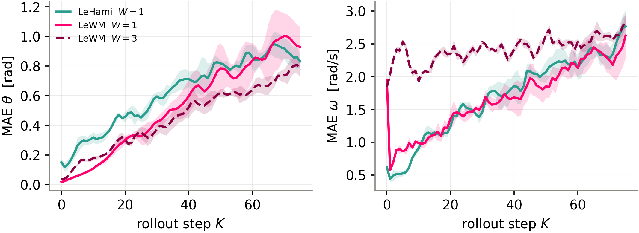
LeHami retains useful velocity information and avoids measured latent-volume loss. Some angle-prediction results favor LeWM, especially early in the driven rollout. The derivative channel contributes information unavailable to a single-frame encoder. These results support the combined state construction and predictor; they do not prove that symplecticity alone recovers every physical quantity.
| model | probe | MAE [ rad] | MAE [rad/s] | |
|---|---|---|---|---|
| LeHami | ridge | |||
| 25-NN | ||||
| MLP | ||||
| LeWM | ridge | |||
| 25-NN | ||||
| MLP |
3.3 LeHami is a world model with time re-stepping and reversal
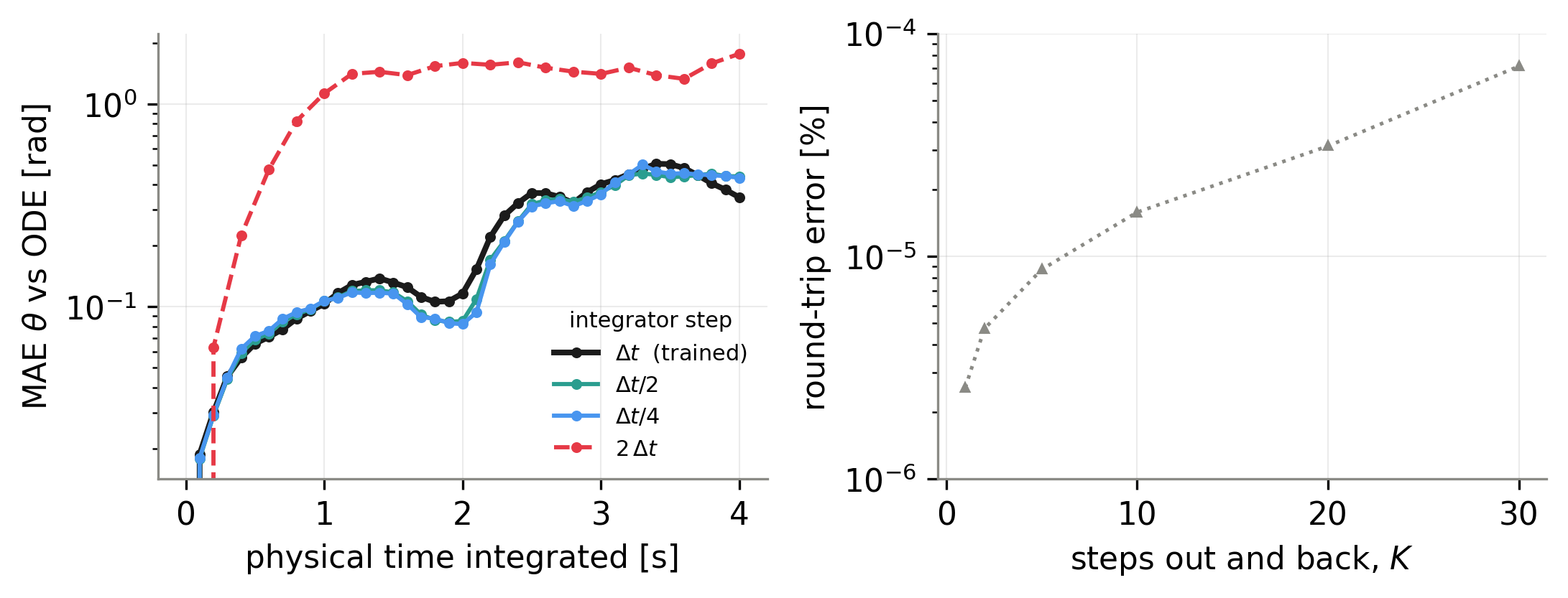
The learned vector field can be integrated at smaller sub-frame steps, and forward/backward integration has small numerical round-trip error. Doubling the step breaks the demonstrated prediction. Symplecticity is an exact algebraic property of the update, while prediction accuracy and stability remain step-size dependent. Reversing an action-conditioned rollout also requires reversing the applied action schedule.
3.4 LeHami brings computational efficiency and structural priors in velocity planning
Under the reported fifteen-TFLOP episode budget, the cheaper predictor permits more frequent replanning. LeHami captures velocity direction better than single-frame or time-symmetric baselines. An untied temporal encoder nevertheless achieves the strongest success rates, and LeHami’s joint position–velocity success is limited by reaching the target angle. The claim is a useful structural and compute tradeoff, not universal planning dominance.
| Clause | Model | Success | TFLOP | Replanning interval |
|---|---|---|---|---|
| Position | LeWM | 12.87 | , 4 solves | |
| LeWM (tied) | 13.65 | , 4 solves | ||
| LeWM (untied) | 13.65 | , 4 solves | ||
| LeHami | 8.05 | , 4 solves | ||
| Velocity | LeWM | 8.78 | , 2 solves | |
| LeWM (tied) | 13.65 | , 4 solves | ||
| LeWM (untied) | 13.65 | , 4 solves | ||
| LeHami | 10.98 | , 5 solves | ||
| Position and Velocity | LeWM | 12.87 | , 4 solves | |
| LeWM (tied) | 9.31 | , 2 solves | ||
| LeWM (untied) | 13.65 | , 4 solves | ||
| LeHami | 10.98 | , 5 solves |
4 Conclusion
The study shows how a mechanical constraint can prevent particular latent rollout failures and supply a useful motion-aware state. The guarantee and the empirical advantage have different scopes: the map preserves volume by design, while physical accuracy and planning quality depend on learning, representation and task.
Limitations and future work.
Strong friction contracts physical phase space and conflicts with the pure volume-preserving prior. Configuration-dependent mass also challenges the fixed derivative-as-momentum construction. Dissipative extensions and learned momentum states are proposed directions, not evaluated solutions. Static pose tasks may benefit less from this extra structure.
AI use statement
The source discloses AI assistance with writing, code and proof checking, while retaining author responsibility for the scientific content.
Ethics statement
The authors describe the work as foundational research without a specific immediate societal application.
Acknowledgements
The source acknowledges guidance and feedback on the research and experiments.
Reproducibility statement
The release records configurations, seeded data generators, episode splits, checkpoint selection and evaluation scripts. Reproduction should follow those artifacts, especially derivative windows, probe fitting and the planning budget. Some supplementary comparisons use one seed, unlike the main three-seed results.
Appendix A Appendix organization
The appendices separate mathematical guarantees, architectural choices, data generation, evaluation and supplementary results. This distinction is useful: a proved map property is not the same as a measured physical capability.
Appendix B Background in Hamiltonian mechanics
Hamiltonian dynamics evolve a paired position–momentum state using derivatives of one scalar function. In physical mechanics that function is energy; here the learned scalar mainly supplies a geometric restriction on latent evolution. It need not equal the environment’s physical energy.
Equation 6
| (6) |
Phase-space density.
Following a cloud of initial conditions under Hamiltonian flow preserves its density along motion. This is an incompressibility statement in the full phase space, not a claim that each coordinate or projected picture stays unchanged.
Symplectic form.
The symplectic form tracks oriented areas across paired coordinates. Preserving this structure implies full phase-space volume preservation. Projected areas or individual distances can still change.
Appendix C Theory
C.1 Symplecticity of the leapfrog step: formal statement and proof
The proof decomposes leapfrog into invertible momentum and position shears. Their symmetric Hessians make each shear symplectic; composition retains that property. With twice continuously differentiable generator terms and an action held fixed within each step, the Jacobian determinant is one. Thus distinct states remain distinct, uniform contraction is impossible and a fixed point cannot attract an open neighborhood. This is exact-arithmetic structure; finite precision introduces numerical error.
Equation
Proposition 2 (Formal form of Proposition 1).
Let and , and let be the leapfrog step of Eq. equation 4 generated by with the control held fixed within the step. This means that the leapfrog step can be written as with
Equation 7
| (7) |
Then is a diffeomorphism of that is exactly symplectic, which means that
Equation 8
| (8) |
for every step size , every control and every parameter . Consequently , Lebesgue measure volume on is -invariant, and for every horizon the three below conditions are met:
- (i)
(no uniform contraction) the singular values of with satisfy , hence at every ;
- (ii)
(no asymptotically stable fixed point) admits no asymptotically stable fixed point, where “asymptotically stable” means: a fixed point that is Lyapunov stable and attracts every point of some open neighbourhood of itself;
- (iii)
(no merging) is a composition of diffeomorphisms, hence itself a diffeomorphism of , in particular injective. Consequently, if then for every : two latents that differ at the anchor remain distinct at every horizon.
Equations
C.2 Scope and limitations of the guarantee
Three limits are essential. Volume preservation does not bound rollout error; an invertible map can still stretch badly. It also does not preserve a Gaussian feature distribution, so encoder regularization remains relevant. Finally, latent Hamiltonian structure does not identify the true physical Hamiltonian or make the encoder injective on physical states. Distinct inputs already merged by the encoder cannot be recovered by an invertible predictor.
Remark 3 (Shape, not size).
A cloud that cannot be squeezed can still be sheared and stretched arbitrarily, so symplecticity places no bound on the growth of rollout error and does not make the rollout accurate. What it removes is the degenerate failure in its three forms: the rollout that shrinks in every direction at once, the one that settles onto an attractor and stops moving, and the one that merges states which started apart.
An unconstrained predictor is under no such constraint, and the one-step objective pushes it the other way. Under any observation or latent noise, the minimiser of is the conditional mean , which averages away whatever the anchor leaves undetermined: it contracts volume, and it sends latents that differ only in the averaged-out directions to a common image. Volume loss and merging are therefore the trained optimum for such a map and iterating it drives the rollout onto exactly the attracting set the proposition forbids for . The proposition says the Hamiltonian rollout cannot enter that regime at any step size , any parameter or any horizon.
Remark 4 (Regularization is not made redundant).
Proposition 1 states that the flow carries phase-space volume exactly and its does not state nothing about the shape of the distribution that volume belongs to. Due to this, regularization techniques are not made redundant. In this work, we leverage the SIGReg (Balestriero and LeCun, 2025) as regularizer, as it is the one used in LeWM and has shown state-of-the-art performance (Maes et al., 2026b). For the isotropic Gaussian installed by SIGReg at the encoder to be invariant under the flow, the radius would itself have to be a conserved quantity of the generator, that is . This is a genuine restriction: it is a functional constraint on , not a consequence of symplecticity, and a general learned Hamiltonian, which is action-conditioned, and parameterised by free-form networks as we do here, has no reason to satisfy it.
The two mechanisms are therefore complementary rather than substitutes. SIGReg shapes the encoder distribution, during training and in expectation over batches, which is where a collapse of the representation would originate. Symplecticity carries the volume of whatever distribution it is handed, at every inference step and for every input, which is where an iterated map would otherwise contract or explode.
Remark 5 (Geometric prior, no physical modeling).
We are not modeling the physics of the observed system. is never fit to a known Hamiltonian and is not claimed to recover one: the true equations of motion enter only as evaluation targets for frozen read-out probes, never as a training signal. This is the point of departure from Hamiltonian neural networks (Greydanus et al., 2019) and SRNN (Chen et al., 2019), where the learned is a surrogate for the physical Hamiltonian and recovering it is the goal.
The prior models the latent representation space. Writing for the maps a JEPA predictor may realize, we restrict it to the symplectomorphisms reachable as one leapfrog step of a learned separable generator ; the content of that restriction is geometric (Proposition 1), and it governs the dynamics, or evolution, latent space. The canonical split is structural in the same sense: the encoder emits with and the flow operates on that split by construction, but is not assumed to encode position, nor momentum, in any observation-space sense.
C.3 Why Hamiltonian and not Lagrangian
A separable Hamiltonian permits cheap explicit first-order updates on a paired state through leapfrog. This is the implementation reason for choosing it over a second-order Lagrangian formulation. The choice does not make the two physical formalisms inequivalent.
C.4 Design choices in the flow and the encoder
Actions enter the potential and stay constant during each integration step. The derivative stencil is causal for input anchors and centered only for training targets, which never feed the rollout. Defining momentum as the derivative of learned position fixes a useful coordinate convention, but it is not a general derivation of canonical physical momentum. Constant-mass systems can fit this convention; configuration-dependent mass can make the separable model misspecified. The learned scale and alternative SIGReg placements affect optimization without replacing the geometric guarantee.
Equations 9–12
| (9) |
| (10) |
| (11) |
| (12) |
Appendix D Description of the experimental set up
D.1 Methodology
Comparisons share data, clipping, optimizer and the total latent width, while LeHami splits that width into two halves. Checkpoints use validation data. This controls several confounds, but the derivative state and predictor both change together.
D.2 Implementation of LeHami
The implementation uses smooth MLP generator terms and fixed derivative stencils. The same causal derivative initializes training, evaluation and planning; centered targets provide lower-noise supervision. Once rollout begins, no new stencil or image supplies its state. Mixed-recording-rate training is described as an architectural possibility and explicitly was not tested.
D.3 Datasets and their architectures
D.3.1 Conservative pendulum.
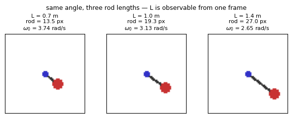
The conservative dataset varies length and includes oscillating and rotating trajectories. Only the stated single-frame-rate slice is used in the main experiment. Rendered rod length is visible from an image, making it a useful system-parameter control.
Equation 13
| (13) |
D.3.2 Action as a force: actuated pendulum.
The driven dataset varies length and mass and holds torques over three frames. Drive changes energy while retaining the volume-preserving dynamics used by the model. This is different from frictional energy loss.
Equation 14
| (14) |
D.3.3 The data split protocol
Whole episodes are split into training, validation and test, stratified by system-parameter combinations. Overlapping clips are drawn only after that split, preventing shared episode frames across partitions.
| conservative pendulum | actuated pendulum | |
| episodes used | 300 | 900 |
| frames per episode | 80 | 80 |
| s | s | |
| split, in episodes (train / val / test): | ||
| episodes | ||
| design cells | 3 rod lengths | 9 () |
| episodes per cell | 100 | 100 |
| train episodes per cell | 70 | 70 |
D.4 Evaluation
The evaluation uses physical readout probes and executed simulator trajectories, with separate metrics for representation quality and control.
D.4.1 The probes
Angle is read as sine and cosine and converted back with atan2, avoiding a spurious discontinuity at a full turn. Probes fitted after one step help compare models with different access to motion history. Linear and nonlinear probes reveal different degrees of decodability.
D.4.2 Planning
Only the driven pendulum has actions to optimize. The controller uses encoded start context and a supplied goal window; physical state is reserved for scoring.
Goal construction.
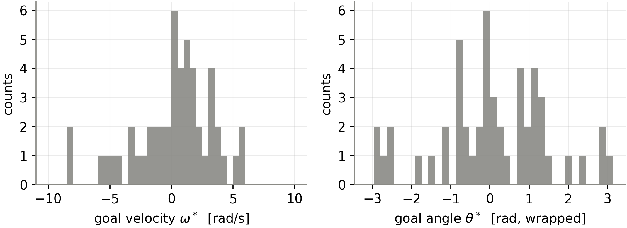
Goals are actual later states from held-out episodes, making them reachable under some action sequence. This controls impossible targets, but the benchmark still supplies an informative target observation and motion window.
Latent states, and the frames they are read from.
Start and goal latents use the frames each architecture needs. LeHami’s goal includes history-derived momentum, while a single-frame baseline goal cannot directly specify velocity. Temporal-window variants address that difference.
Optimisation.
CEM ranks action candidates by terminal latent distance. Replanning shrinks the remaining horizon toward a fixed goal time and uses newly observed context. This avoids continually moving the deadline into the future.
No leakage.
Intermediate imagined states are self-fed. The source states that future episode states and recorded future actions do not initialize or rank candidate plans. Replanning contexts contain only observations already available to the controller.
Scoring success.
Success is measured at the target time using separate angle and signed-velocity tolerances. Angle differences are wrapped on the circle. Temporal encoder lag is accounted for when building online contexts. Passing near the goal at any earlier time is a different and easier criterion.
Equation 15
| (15) |
Settings.
The protocol fixes a thirty-frame goal horizon, action bounds and a CEM budget, then sweeps replanning frequency. Results combine model and planner seeds on the same fifty goals. FLOP limits constrain which feedback rates can be compared.
Appendix E Supplementary experimental results
The supplementary experiments vary encoder design, regularization, prediction horizon and planning feedback. They explain both the observed improvements and the remaining failure cases.
E.1 LeHami replaces manual design choices with structural priors and lower compute
A time-symmetric encoder can recover speed while discarding its sign: reversing its frame window leaves the feature unchanged. An asymmetric derivative or untied temporal weights preserve that distinction. LeHami improves compute-to-error performance in the reported conservative-pendulum study, but that training-compute comparison uses one seed per model.
| Metric | Model | PFLOP | PFLOP | PFLOP | PFLOP |
|---|---|---|---|---|---|
| MAE [rad] | LeHami | (ep 9) | (ep 19) | (ep 39) | (ep 79) |
| LeWM | 0.590 (ep 9) | 0.871 (ep 19) | 0.487 (ep 39) | 0.321 (ep 79) | |
| MAE [rad/s] | LeHami | (ep 9) | (ep 19) | (ep 39) | (ep 79) |
| LeWM | 1.625 (ep 9) | 2.146 (ep 19) | 1.620 (ep 39) | 1.270 (ep 79) |
| Model | Total | Encoder | Predictor | Projector | Pred. proj. |
|---|---|---|---|---|---|
| LeHami | 3.03 | 0.315 | 2.234 | 0.465 | — |
| LeWM | 4.44 | 0.315 | 3.310 | 0.530 | 0.268 |
| LeWM | 4.45 | 0.318 | 3.310 | 0.530 | 0.268 |
E.2 Conservative pendulum
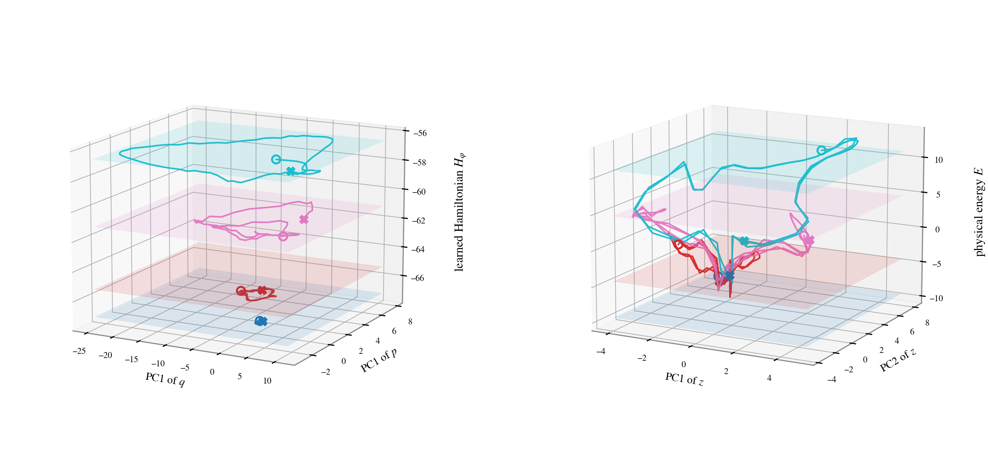
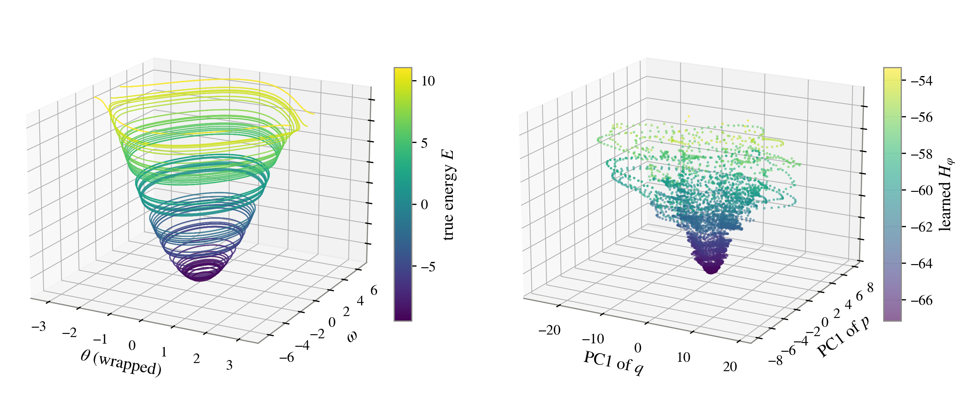
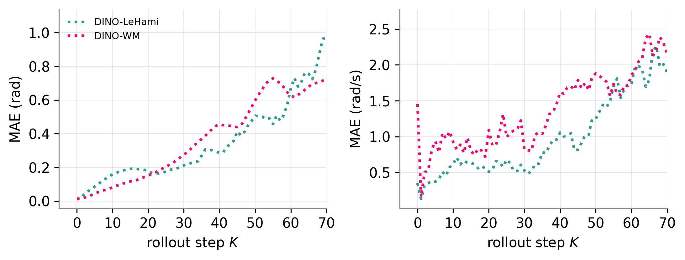
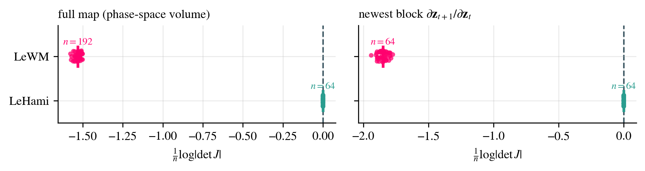
Latent plots illustrate structured orbits, while probes test whether physical information remains decodable. Energy-like organization and unit Jacobian determinant do not ensure accurate long-rollout coordinates: the model’s momentum features drift from their encoded targets. The full three-state context map is used to assess LeWM volume, since its newest-output block alone is not a complete state-transition map. Some frozen-encoder controls use a separate single-length dataset and one seed.

| rollout step | 0 | 1 | 5 | 10 | 20 | 25 | 50 |
|---|---|---|---|---|---|---|---|
| (position block) | |||||||
| (momentum block) |
| MAE [rad, wrapped] | MAE [rad/s] | |||||
| band | LeHami | LeWM | ratio | LeHami | LeWM | ratio |
| – | 0.107 | 0.100 | 0.93 | 0.364 | 1.020 | 2.80 |
| – | 0.225 | 0.287 | 1.27 | 0.669 | 1.169 | 1.75 |
| – | 0.596 | 0.981 | 1.65 | 1.534 | 2.331 | 1.52 |
| anchor (), from the frozen encoder features: LeHami LeWM | ||||||
| same anchor, LeHami read by the linear tier: ridge , against the 25-NN’s above | ||||||
E.3 Actuated pendulum
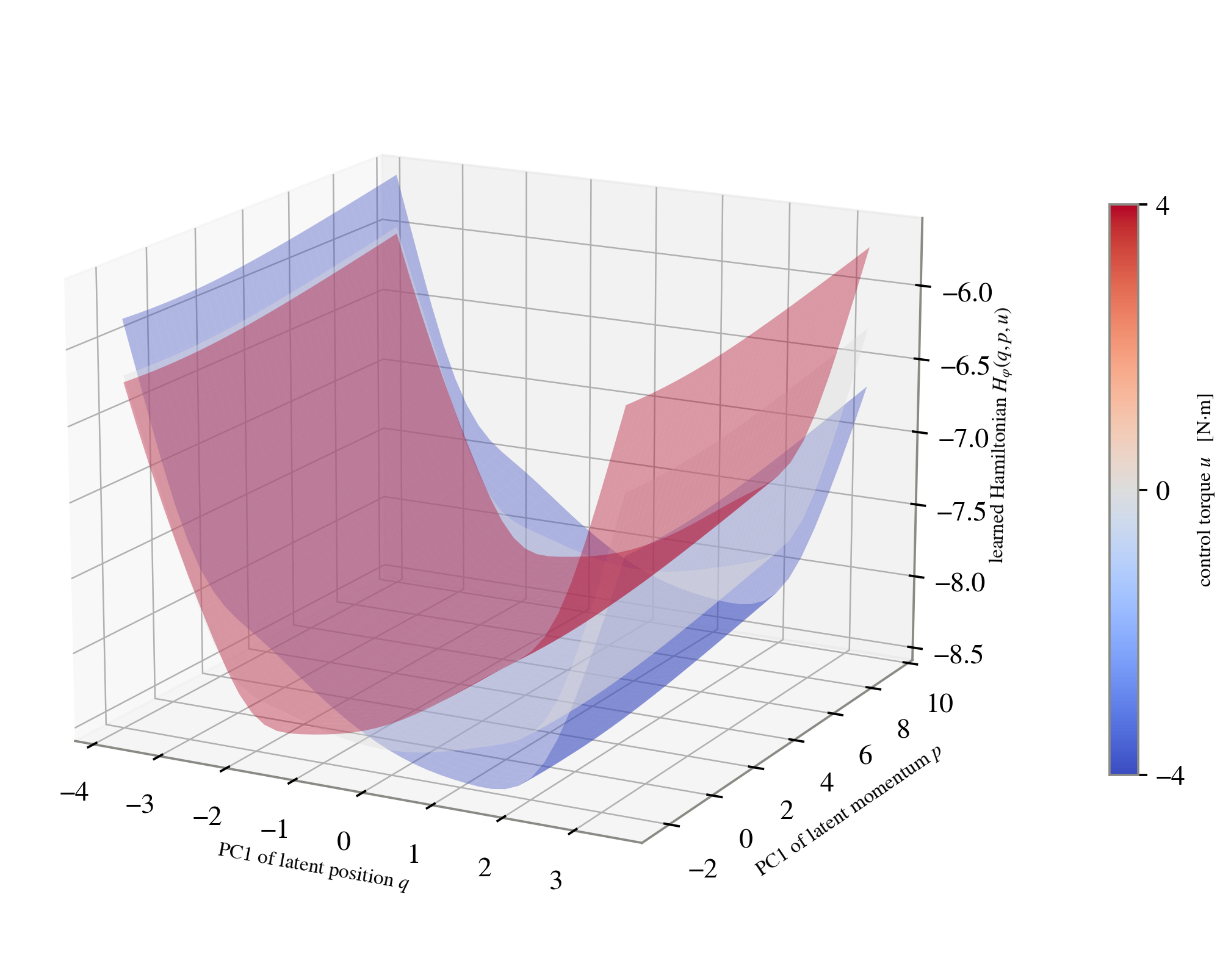
Driving changes the learned energy along a trajectory without removing symplecticity. Joint Gaussian regularization can hide a nearly inactive momentum block by inflating position variance; placement therefore matters. A symmetric temporal baseline confuses opposite velocity signs, whereas untied weights correct that failure. Both model families retain mass and length, so those system parameters do not explain the control gap.
| window | SIGReg | within-episode % | |||
|---|---|---|---|---|---|
| joint | 1.356 | 0.006 | 0.0043 | ||
| q | 0.980 | 0.101 | 0.1031 | ||
| split | 1.174 | 0.236 | 0.2014 | ||
| joint | 1.405 | 0.051 | 0.0362 | ||
| q | 0.979 | 0.051 | 0.0519 | ||
| split | 1.124 | 0.201 | 0.1784 |
Equation 16
| (16) |
| Model | gap | |||
|---|---|---|---|---|
| LeWM | 3 | |||
| LeWM | 3 |
Planning compute.
Compute savings come mainly from cheaper predictor rollouts. LeHami improves velocity direction relative to passive coasting and symmetric baselines, but the untied baseline performs better overall. Conditioning joint success on reaching the angle shows that position control is LeHami’s main bottleneck here. Recoverable mass and length do not imply every latent coordinate remains linearly calibrated.
| Clause | Model | Success | TFLOP | Replanning Interval () |
| Velocity, magnitude | LeWM | 8.78 | , 2 solves | |
| LeWM (tied) | 13.65 | , 4 solves | ||
| LeWM (untied) | 13.65 | , 4 solves | ||
| LeHami | 10.98 | , 5 solves | ||
| coast | 0.300 | — | — | |
| Velocity, sign | LeWM | 5.85 | , 1 solve | |
| LeWM (tied) | 13.65 | , 4 solves | ||
| LeWM (untied) | 13.65 | , 4 solves | ||
| LeHami | 8.05 | , 4 solves | ||
| coast | 0.680 | — | — |
| rod length | bob mass | ||||
|---|---|---|---|---|---|
| probe | model | ||||
| ridge | LeHami | 0.999 | 0.900 [0.871, 0.951] | 0.999 | 0.977 [0.958, 0.993] |
| LeWM | 0.999 | 0.983 [0.976, 0.990] | 0.999 | 0.993 | |
| -NN | LeHami | 1.000 | 0.997 [0.992, 1.000] | 1.000 | 1.000 |
| LeWM | 1.000 | 1.000 | 1.000 | 1.000 | |