Overview
At a glance
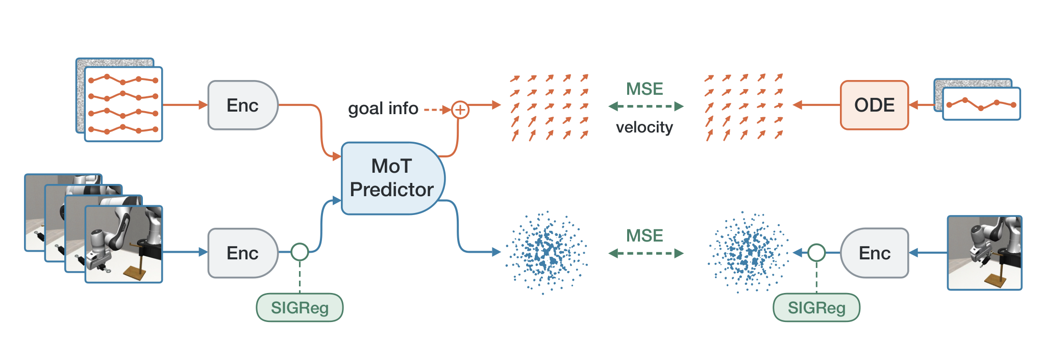
LeWAM jointly trains a visual encoder, action-conditioned latent dynamics, and an action flow-matching policy from reward-free offline trajectories. Predicting both future states and actions encourages control-relevant representations; SIGReg keeps the latent distribution diverse.
The same architecture supports direct action sampling or goal-image planning that refines learned action proposals through the dynamics model. Across ten simulated planning tasks it averages 93.5% success versus LeWM's 50.9%; a separate four-task timing comparison reports 32.3× higher mean planning throughput. Physical-robot experiments use direct policy execution, without online planning.
1 Introduction
Latent world models avoid expensive pixel prediction, but their representations can retain distracting visual information and their planners can waste samples on ineffective actions (Sobal et al., 2022). Adding a policy only after freezing the representation disconnects action supervision from perception.
LeWAM learns perception, consequences, and behavior together. Its roughly 17M-parameter simulated model uses a joint state/action objective plus one latent-regularization weight. A learned action distribution supplies useful proposals, while gradients through predicted consequences refine them toward a visual goal.
2 Related Work
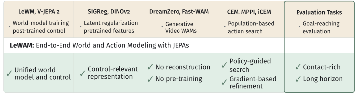
Unlike pixel-generating world models, JEPAs predict representations (LeCun, 2022). DINO-WM uses pretrained visual features; LeWM learns them with SIGReg (Zhou et al., 2024) (Maes et al., 2026b). LeWAM adds joint policy learning so action supervision also shapes the encoder.
GC-IDM and PRISM learn action predictors on frozen world-model features (Nguyen et al., 2026) (Wang et al., 2026). LeWAM instead trains clean-action dynamics and noisy-action flow matching on the same sample and forward pass. Unlike video/action generative approaches, its training needs neither reward labels nor pixel reconstruction.
3 Methodology
Training data are offline image-and-action trajectories. The model predicts future image representations and a distribution of action chunks, supporting goal-conditioned planning or goal-free behavior cloning.
3.1 End-to-End Training with LeWAM
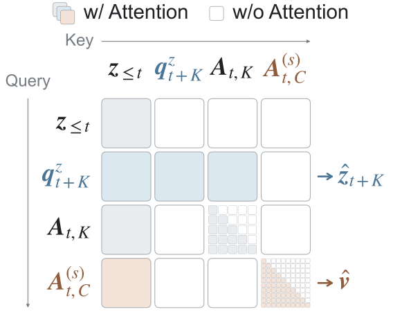
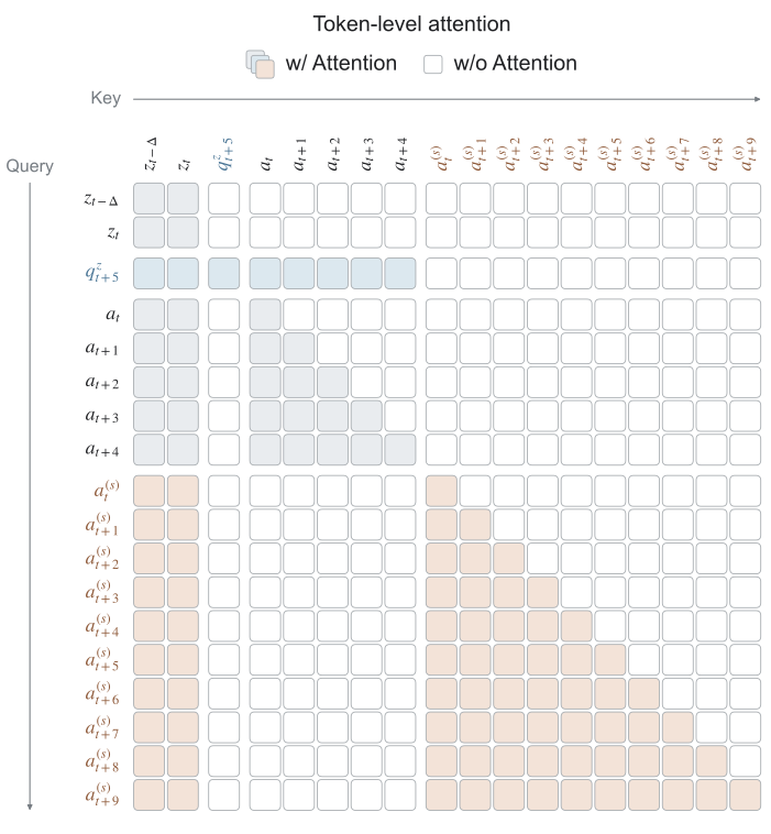
A shared ResNet-18 encoder with spatial softmax produces visual latents. A MoT predictor has separate state and action projections but shared masked attention. Its state query reads history and clean recorded actions; noisy action tokens read history and their own causal prefix. History cannot read clean actions, preventing indirect target leakage across layers.
The policy predicts a contiguous C-action chunk while dynamics targets are K environment steps apart. Optional goal context includes a goal-image latent and remaining horizon, visible only to noisy action tokens. Flow matching regresses the velocity from Gaussian noise to recorded actions; dynamics regresses the encoded future state.
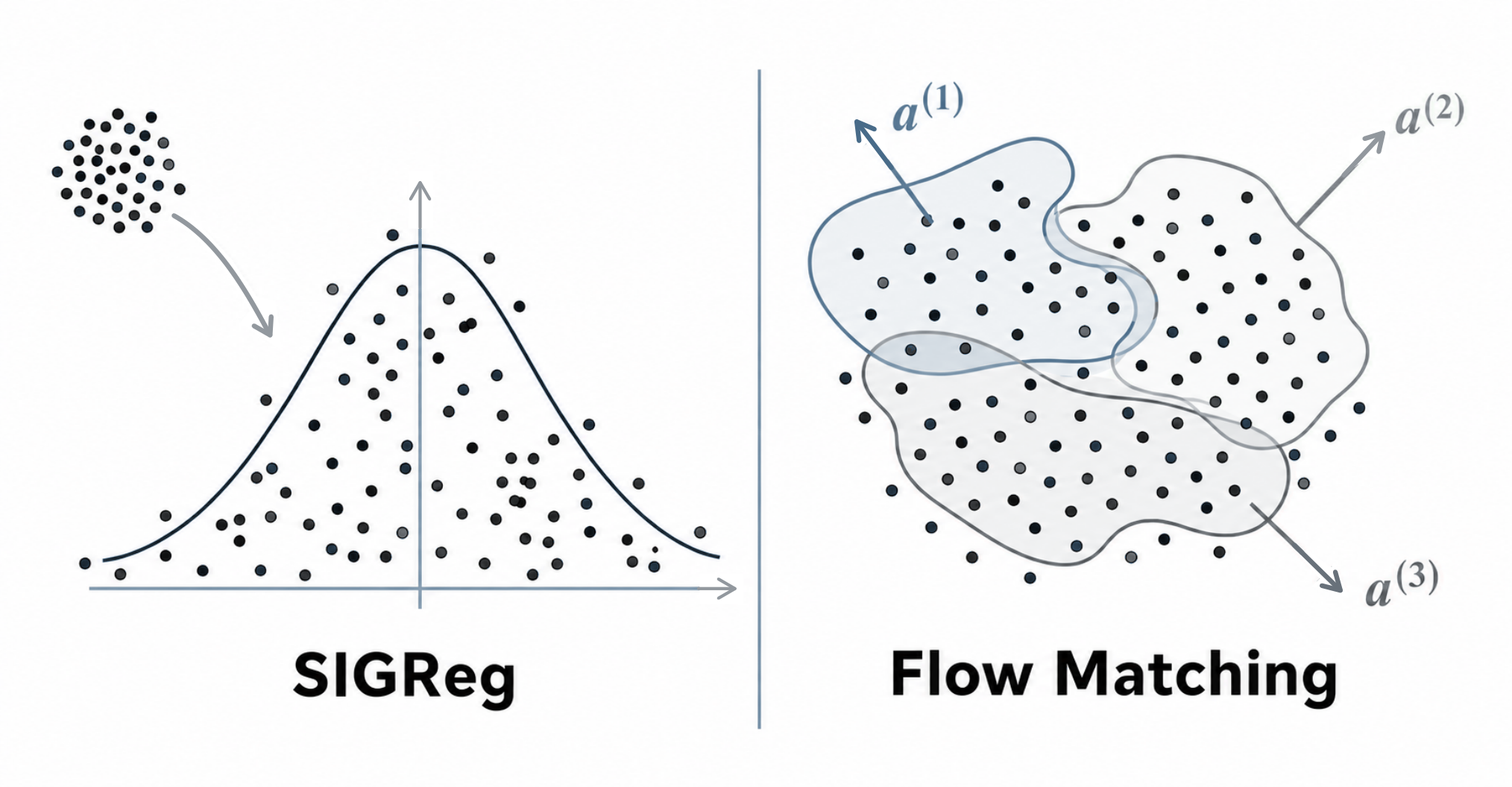
The total loss adds the two coordinate-averaged MSE terms and SIGReg with weight λ. SIGReg uses one-dimensional normality tests on random latent projections to encourage a standard isotropic Gaussian distribution (Balestriero and LeCun, 2025).
Equations 1–5
| (1) | ||||
| (2) |
| (3) | ||||
| (4) |
| (5) |
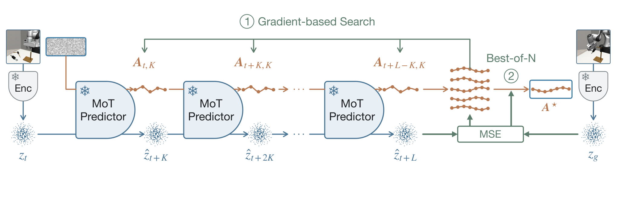
3.2 Efficient Control with LeWAM
Direct control integrates the action flow from Gaussian noise, executes the first K actions, and samples again after observing the result.
Planning first generates N candidate sequences by alternating action sampling and predicted-state updates. It then differentiates terminal latent distance to the goal through the learned dynamics to refine each sequence. A small proximity penalty discourages large departures from the sampled plans. The lowest unpenalized goal-cost iterate is selected; only its first K actions execute before replanning.
Equations 6–8
| (6) |
| (7) |
| (8) |
4 Experiments
Experiments separate visual-goal planning, diagnostic analysis of learned representations and dynamics, and goal-free behavior cloning in simulation and on physical robots.
4.1 Evaluation Protocol
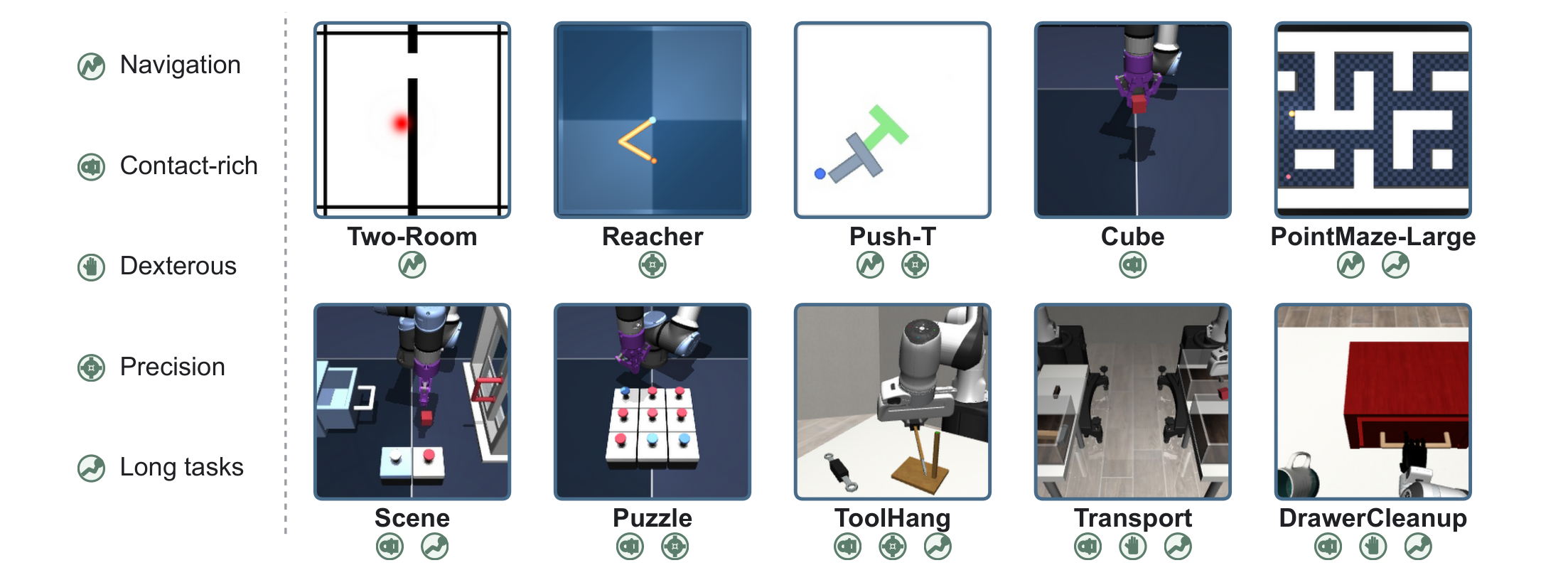
Ten simulated tasks span navigation and contact-rich manipulation using expert, random, and mixed-quality trajectories. Visual planning receives a goal image and a fixed action budget. Task completion instead learns one demonstrated behavior without a goal image. Within each protocol, methods share observations, action limits, goals, budgets, and success criteria.
4.2 Visual Planning with LeWAM
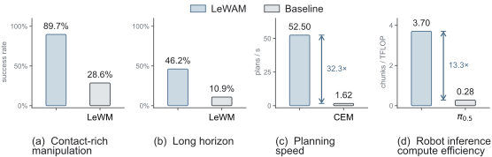
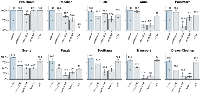
Against LeWM with CEM, LeWAM improves mean success from 50.9% to 93.5% over ten tasks and wins every task. Contact-rich task averages rise from 28.6% to 89.7%, including ToolHang 35.4→94.7% and Transport 2.8→83.3%.
On four tasks with goals 100 steps after the start, the same checkpoints achieve 46.2% mean success versus 10.9%. These longer goals are distinct from the default short-horizon benchmark.
On an H100, mean per-task planning throughput is 52.50 versus 1.62 plans/s, a reported 32.3× ratio. This compares five gradient updates with LeWM's 300-candidate, 30-iteration CEM; it is planner-call timing, not an end-to-end robot-control speedup.

4.3 Understanding LeWAM’s Dynamics, Representations, and Actions
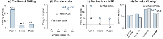
Linear probes find more decodable proprioception and actions in jointly trained representations. Without SIGReg, latent-only LeWM collapses on the reported Push-T probes, while action-supervised variants retain information. Action supervision alone is insufficient for the strongest planning: SIGReg also improves object information and goal sensitivity.
Across four tasks, direct success averages 86.7% with a jointly trained encoder, versus 79.0% with frozen DINOv2 CLS features and 75.8% with frozen patch features. A stochastic flow head gives larger planning gains than a deterministic MSE head with added Gaussian noise. Distribution modeling can distinguish histories whose action means match but whose valid behaviors differ.
| Environment | Model | SIGReg | Eff. rank | Object | Proprio | Action (IDM) |
|---|---|---|---|---|---|---|
| Push-T | LeWAM | Yes | ||||
| No | ||||||
| LeWAM (MSE) | No | |||||
| LeWM | Yes | |||||
| No |
Isolating Action-Conditioned Dynamics.
Removing the action head at evaluation and planning with CEM isolates learned dynamics. LeWAM remains competitive on Push-T and improves Cube success by 22.2 points over LeWM. Decoded recorded-action rollouts also show clearer control-relevant details on the three-dimensional tasks; these diagnostics use separate post-trained pixel decoders.
4.4 Behavior Cloning and Physical Robot Control
Goal-free LeWAM directly executes sampled action chunks. On DrawerCleanup, Transport, and ToolHang it is competitive with Diffusion Policy, improving Transport by 16 points (Chi et al., 2023).
Physical experiments compare LeWAM trained from scratch, a frozen V-JEPA 2.1 variant, Diffusion Policy, and π0.5 on three tasks. All train or adapt on the collected teleoperation demonstrations and execute half of each action chunk. LeWAM is competitive; its two encoder variants have similar average success. Each method receives 30 trials per task, and no physical experiment uses online planning.

| Method | Pick and Place T | Push-T | Tape Stack | Average | GFLOPs |
|---|---|---|---|---|---|
| Diffusion Policy (Chi et al., 2023) | 0/30 | 38.9% | |||
| (Physical Intelligence et al., 2025) | 3/30 | 9/30 | 28.9% | ||
| LeWAM (Frozen V-JEPA 2.1 Encoder) | 5/30 | 35.6% | |||
| LeWAM | 6/30 | 33.3% |
5 Conclusion and Limitations
Joint state and action prediction supports useful latent dynamics, learned planning proposals, and direct control. Evidence remains limited to the tested data and tasks: models are trained or adapted separately for each task and embodiment.
Open directions include broader contact-rich play data, unfamiliar objects and viewpoints, multitask and language-conditioned training, hierarchical subgoals, and scaling models or test-time search. The reported results do not establish a universal cross-robot policy.
Reproducibility statement
Architecture, training, data, and evaluation settings are supplied in the appendices, with project and code links in the original paper.
Ethics statement
The authors report no new human-subject data. Reused resources retain their licenses, and physical deployment requires independent safety mechanisms.
AI use statement
Language-model assistants helped polish the manuscript. The authors retain responsibility for the research, analysis, and text.
Appendix A Implementation Details
Simulation uses two history latents, dynamics stride K=5, and ten-action chunks. History stride is five for goal reaching and one for task completion. The encoder maps spatial-softmax features to 192 dimensions; the predictor has four blocks and four heads, totaling 16.9M trainable parameters. Action sampling uses eight Euler steps.
Targets use the online encoder, without a momentum encoder or state noise. SIGReg uses 1,024 projections, 17 knots, and weight 0.04. Visual planning trains 50 epochs at batch 128; goal-free cloning trains 120 epochs at batch 64. Checkpoints minimize validation action flow loss, not task success.
Separate branch parameters share one masked attention operation. Goal and flow-time conditioning affect noisy action tokens. The explicit mask below blocks clean-action leakage into history and the action flow, while letting the future-state query read recorded actions.
Equations 9–10
| (9) |
| (10) | ||||||
A.1 LeWAM Planning
Only normalized candidate actions receive gradients during planning; model weights are frozen. Adam uses learning rate 0.05 and gradient clipping at 10. Updates include a 0.01 quadratic proximity penalty and clip normalized actions to ±3, but candidate retention and final selection use the unpenalized goal cost.
Equation 11
| (11) |
A.2 Baseline Implementations
Baselines share environment wrappers and evaluation interfaces from stable-worldmodel (Maes et al., 2026a). LeWM-IDM freezes a separately trained world model; LeWM-CEM follows its released recipe. DINO-WM compares patch and CLS tokenization, using ten epochs on the six added tasks. GCBC uses frozen DINOv2 features and 20 training epochs.
The simulated Diffusion Policy baseline uses a ResNet-18 encoder per camera and a convolutional U-Net. It predicts 16 actions, executes eight, and samples with 100 DDPM steps. Training uses 120 epochs, a 90/10 window split, and validation denoising loss for selection. Each checkpoint is evaluated on 50 episodes for each of three seeds.
Appendix B Benchmarks and Evaluation
B.1 Tasks and Datasets
The suite retains Two-Room, Reacher, Push-T, and Cube, then adds PointMaze-Large, Scene, Puzzle, ToolHang, Transport, and DrawerCleanup. Data range from random or noisy navigation and interaction to scripted or human demonstrations. Scene and Puzzle use newly collected scripted-oracle trajectories; the complex manipulation tasks use robomimic or DexMimicGen demonstrations.
Task-focused demonstrations broaden contact complexity but constrain the diversity of visual goals. Table 3 retains action dimensions, views, and dataset scale; synchronized cameras count once toward duration.
| Task | Collection regime | Views | Dim. | Traj. | Mean frames | Total frames | Hz | Hours |
|---|---|---|---|---|---|---|---|---|
| Two-Room | Noisy heuristic | 1 | 2 | 10,000 | 92 | 920,809 | 10 | 25.58 |
| Reacher | Uniform random | 1 | 2 | 10,000 | 201 | 2,010,000 | 25 | 22.33 |
| Push-T | Non-expert | 1 | 2 | 18,685 | 125 | 2,336,736 | 10 | 64.91 |
| Cube | Scripted expert | 1 | 5 | 10,000 | 201 | 2,010,000 | 20 | 27.92 |
| PointMaze-Large | Scripted navigation | 1 | 2 | 1,000 | 1,000 | 1,000,000 | 10 | 27.78 |
| Scene | Scripted expert | 1 | 5 | 10,024 | 200 | 2,004,800 | 20 | 27.84 |
| Puzzle (33) | Scripted expert | 1 | 5 | 10,024 | 200 | 2,004,800 | 20 | 27.84 |
| ToolHang | Human demos | 1 | 7 | 200 | 480 | 95,962 | 20 | 1.33 |
| Transport | Generated demos | 3 | 14 | 1,029 | 408 | 419,712 | 20 | 5.83 |
| DrawerCleanup | Generated demos | 3 | 24 | 1,026 | 291 | 298,235 | 20 | 4.14 |
| Reported total (10) | 71,988 | 13,101,054 | 235.51 |
B.2 Goals and Success Criteria
Default goal images come 25 recorded steps after the initial state, with 50 executable actions. Two-Room instead uses a 100-step offset and 150-action budget. Results generally average three evaluation seeds and 50 episodes per seed; first-hit success matches the baseline protocol.
Cube now requires both cube and end-effector positions within 0.04 m of their goal positions. The old object-only criterion rewarded doing nothing on 42.7% of short-horizon episodes; the corrected criterion reduces that floor to 2.7%. Blind zero-action and random-policy controls are retained in Table 4.
| Environment | Raw action dim. | 25-step goal reaching | Task Completion | ||
|---|---|---|---|---|---|
| Zero-action | Random | Zero-action | Random | ||
| Two-Room | 2 | ||||
| Reacher | 2 | ||||
| Push-T | 2 | ||||
| Cube | 5 | ||||
| Cube (EEF) | 5 | ||||
| PointMaze-Large | 2 | ||||
| Scene | 5 | ||||
| Puzzle | 5 | ||||
| ToolHang | 7 | ||||
| Transport | 14 | ||||
| DrawerCleanup | 24 | ||||
Darker shading indicates a higher control success rate.
B.3 Planning and Timing Protocols
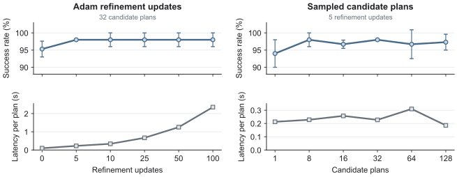
Long-horizon sweeps use the first held-out trajectory frame and goals 25, 50, 75, or 100 steps later. Push-T sensitivity varies gradient updates at 32 candidates, or candidate count at five updates.
Timing measures one planner call on the same H100. Throughput is averaged after converting each task's milliseconds per plan to plans per second. The headline ratio compares LeWM's 300×30 CEM with five LeWAM gradient updates.
Appendix C Additional Results
C.1 Visual Planning Results
Tables 5–6 retain horizon-dependent success and per-call timing. In the tested Push-T sweep, success plateaus after five refinement updates while latency keeps rising; more than eight candidates gives no consistent gain.
| Task | Method | Goal horizon (steps) | |||
|---|---|---|---|---|---|
| 25 | 50 | 75 | 100 | ||
| Push-T | LeWAM | ||||
| LeWM (CEM) | |||||
| Cube | LeWAM | ||||
| LeWM (CEM) | |||||
| Scene | LeWAM | ||||
| LeWM (CEM) | |||||
| Puzzle | LeWAM | ||||
| LeWM (CEM) | |||||
| LeWM (CEM) | LeWAM | |||||
|---|---|---|---|---|---|---|
| Task | Action dim. | ms/plan | plans/s | ms/plan | plans/s | Speedup |
| Scene | ||||||
| Puzzle | ||||||
| Cube | ||||||
| Push-T | ||||||
| Task mean | – | – | – | |||
C.2 Component and Visual-Encoder Ablations
Table 7 compares SIGReg and action heads using epoch-30 checkpoints. Table 8 separately compares encoders. Direct execution has no search; planning adds action refinement through latent dynamics. Encoder results average Push-T, Cube, Scene, and Puzzle equally.
| Environment | Variant | Direct | Planning | Gain (pp) |
|---|---|---|---|---|
| Push-T | LeWAM | |||
| w/o SIGReg | ||||
| MSE action head | ||||
| Scene | LeWAM | |||
| w/o SIGReg | ||||
| MSE action head | ||||
| Puzzle | LeWAM | |||
| w/o SIGReg | ||||
| MSE action head | ||||
| Cube | LeWAM | |||
| w/o SIGReg | ||||
| MSE action head |
| Visual encoder | Mode | Push-T | Cube | Scene | Puzzle | Average |
|---|---|---|---|---|---|---|
| LeWAM (end-to-end) | Direct | |||||
| Planning | ||||||
| Gain (pp) | ||||||
| frozen DINOv2 CLS | Direct | |||||
| Planning | ||||||
| Gain (pp) | ||||||
| frozen DINOv2 patch mean | Direct | |||||
| Planning | ||||||
| Gain (pp) |
C.3 Probing Latent Representations
Ridge-regression probes use a 4,000/1,000-frame train/test split. Object and proprioception scores average R² over their ground-truth variables. Action probes use the current latent; inverse-dynamics probes also use the future latent. Effective rank measures the dimensional spread of representations (Roy and Vetterli, 2007).
| Environment | Model | SIGReg | Eff. rank | Object | Proprio | Action (IDM) |
|---|---|---|---|---|---|---|
| Push-T | LeWAM | Yes | ||||
| No | ||||||
| LeWAM (MSE) | No | |||||
| LeWM | Yes | |||||
| No | ||||||
| Cube | LeWAM | Yes | ||||
| No | ||||||
| LeWM | Yes | |||||
| Scene | LeWAM | Yes | ||||
| No | ||||||
| LeWM | Yes | |||||
| Puzzle | LeWAM | Yes | ||||
| No | ||||||
| LeWM | Yes |
C.4 Visual Reconstructions and Open-Loop Rollouts
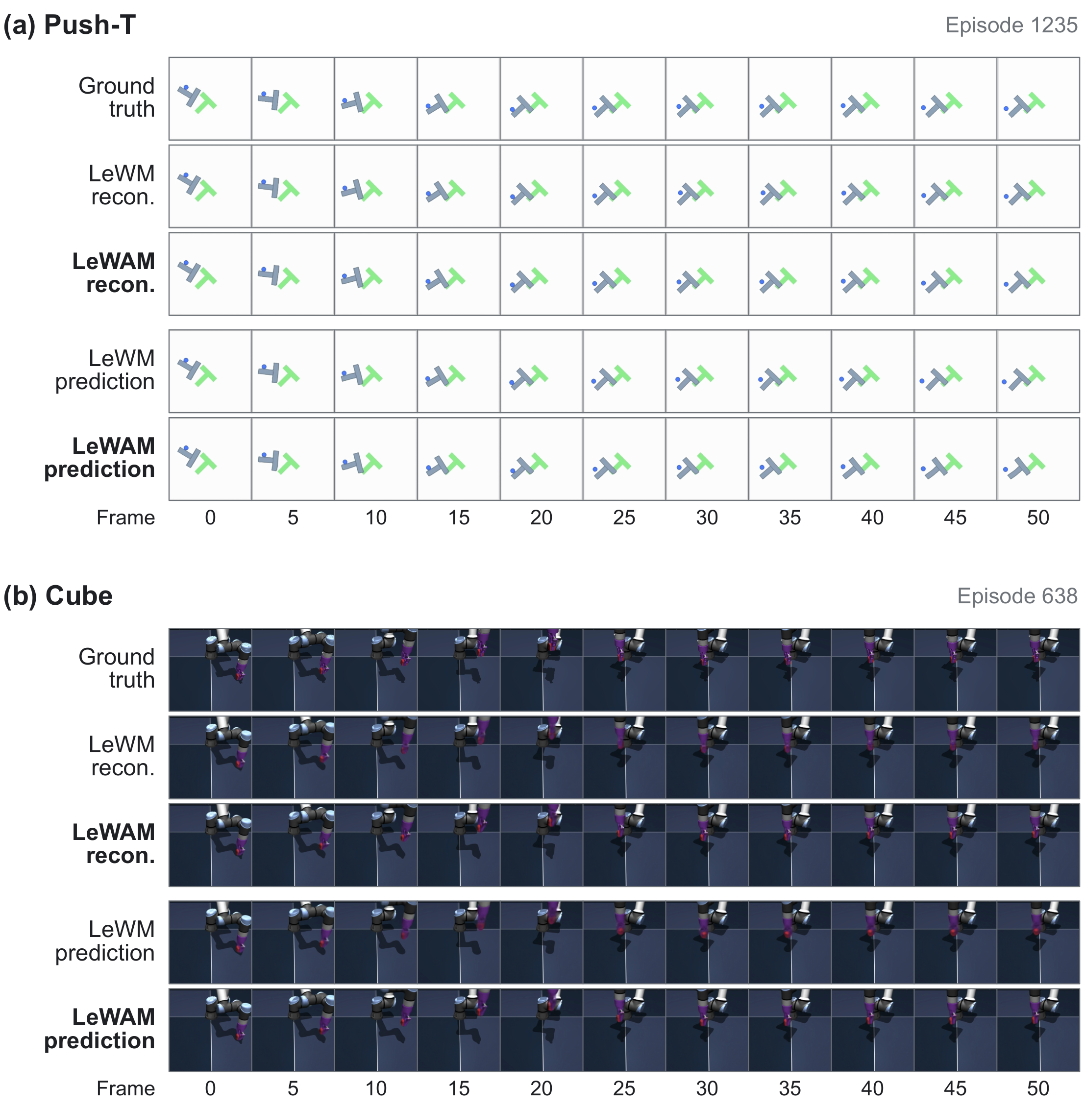
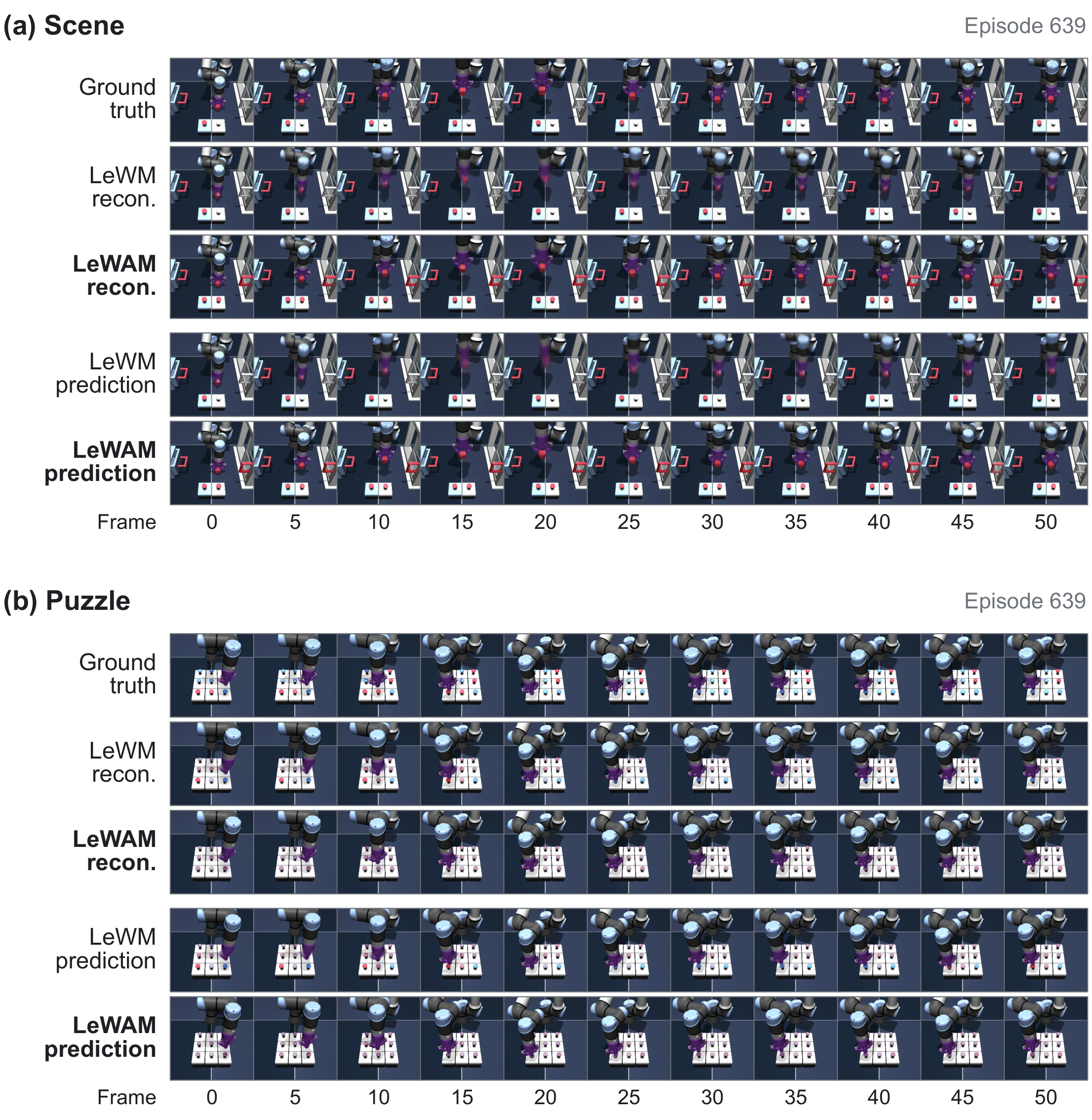
Post-trained pixel decoders visualize frozen representations and open-loop latent rollouts under recorded actions. Displayed clips are excluded from decoder training; each rollout receives only its initial observation context and the fixed recorded action sequence. These are diagnostics, not generated-policy rollouts.
Both models reproduce Push-T motion; LeWAM preserves clearer robot and object details in Cube, Scene, and Puzzle. Encoders, training schedules, and decoders differ between models. Table 10 removes LeWAM's action head and uses CEM, supporting the usefulness of its learned dynamics independently of its policy.
| Model | Push-T | Cube |
|---|---|---|
| LeWM (CEM) | ||
| LeWAM (CEM) |
C.5 Multimodal Action Distributions
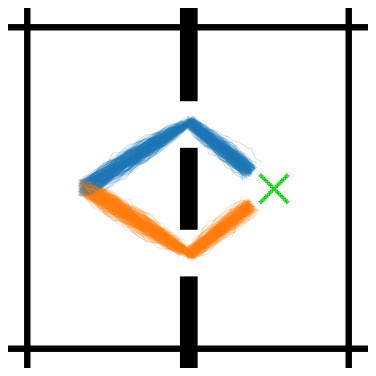
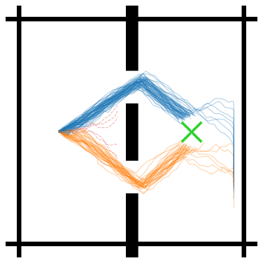
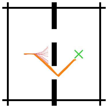
A two-door navigation dataset contains equal upper- and lower-route demonstrations with fixed endpoints. Flow matching preserves both route choices in closed-loop execution; the deterministic MSE head concentrates on the lower route and sometimes hits walls. This illustrates useful multimodal proposals rather than proving coverage of every valid behavior.
C.6 Simulation Task-Completion Results
Table 11 retains per-task behavior-cloning success and deviations for the three goal-free simulated manipulation tasks.
| Method | DrawerCleanup | Transport | ToolHang | Average |
|---|---|---|---|---|
| Diffusion Policy (Chi et al., 2023) | 61.6 | |||
| LeWAM |
Appendix D Physical-Robot Setup and Evaluation
The physical study evaluates direct closed-loop policies trained on task-specific teleoperation data.
D.1 Platform and Data Collection
One proficient operator records successful demonstrations with a reBot Arm 102 leader and B601-DM follower through LeRobot (Cadene et al., 2026). Training uses scene-left and wrist camera crops; the recorded right stereo view is unused. At 30 Hz, recordings include seven joint-target actions and a 21-dimensional position/torque/velocity state. No intentional exploration is collected.
| Task | Episodes | Frames | Duration | Task Description |
|---|---|---|---|---|
| Pick and Place T | 200 | 52,297 | 29 min | ”Pick up the T block and place it onto the outline.” |
| Push-T | 100 | 61,996 | 34 min | ”Push the T block onto the outline.” |
| Tape Stack | 100 | 23,726 | 13 min | ”Stack the green roll of tape on the white roll of tape.” |
D.2 Model Implementation
Both physical LeWAM variants use a ViT-B visual backbone, width 512, eight predictor blocks, and state-MSE plus action-flow losses. One encoder trains from scratch; the other freezes V-JEPA 2.1 features. They take two video context frames and predict three future frames sampled at 2.5 Hz.
Compute in Table 2 counts a complete action chunk: 100 DDPM steps for Diffusion Policy and ten Euler steps for π0.5 and both LeWAM variants. This is an operation count, not measured end-to-end latency.
D.3 Physical-Robot Baseline Configurations
Every physical policy returns 36 actions and executes 18 at 30 Hz, corresponding to 1.2-second predictions and 0.6-second execution intervals. Baselines use the same cameras, seven joint-target actions, and demonstrations.
The stated Pick and Place T/Push-T recipes hold out 10% of episodes and train 20,000 updates at effective batch 256. Diffusion Policy uses per-camera ImageNet-initialized ResNet-18 encoders, a U-Net, 100 sampling steps, and moving-average weights. π0.5 freezes its vision/language backbone and trains its action expert; discretized joint torques enter the language prompt.
D.4 Closed-Loop Evaluation
Observations travel to a remote inference machine; the robot executes returned action chunks at 30 Hz. A human labels success using the demonstration criteria. Each task/method has 30 trials, limiting the precision of small observed differences.
D.5 Representation Diagnostics and Evaluation
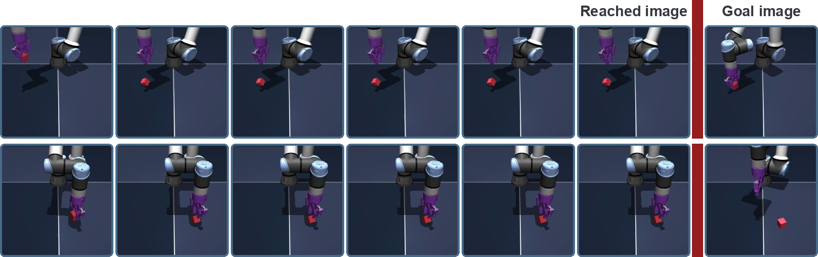
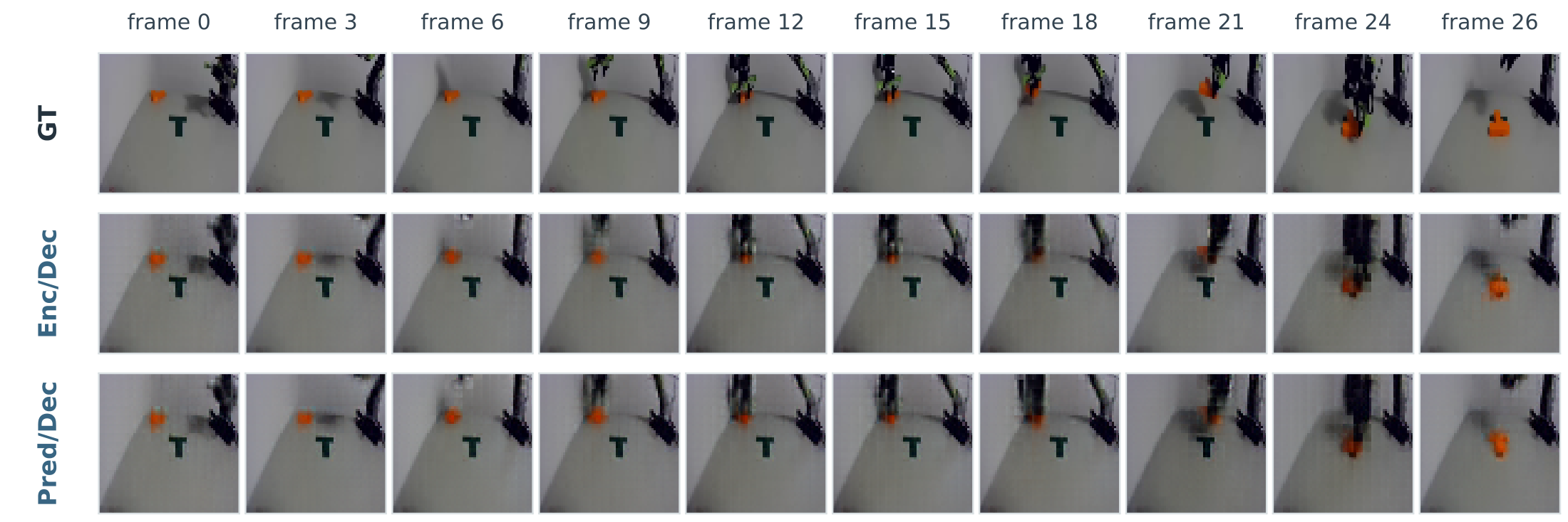
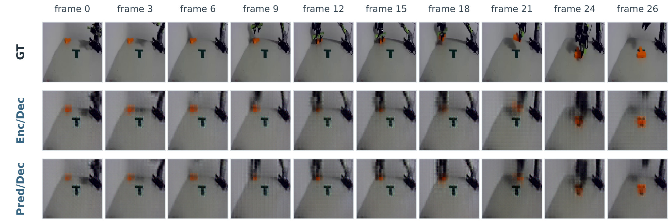
A separately trained pixel decoder maps frozen latents to images. Figure 16 compares the two encoder variants on one held-out Pick and Place T episode: recorded frames, framewise reconstructions, and autoregressive latent predictions. Rollouts follow recorded actions without intermediate ground-truth images or newly generated actions; ten displayed frames span 10.4 seconds.
Equation 12
| (12) |
Appendix E Discussion of the Role of Joint Prediction
The appendix explains how joint prediction can shape representations and improve proposal quality. Table 13 compares training requirements and capabilities across related models.
| Method | FDM | Policy | Joint FDM and Policy | End-to-end from scratch |
|---|---|---|---|---|
| World models | ||||
| DINO-WM (Zhou et al., 2024) | ✓ | ✗ | ✗ | ✗ |
| V-JEPA 2-AC (Assran et al., 2025) | ✓ | ✗ | ✗ | ✗ |
| LeWM (CEM) (Maes et al., 2026b) | ✓ | ✗ | ✗ | ✓ |
| World action models | ||||
| UVA (Li et al., 2025) | ✓ | ✓ | ✗ | ✗ |
| UWM (Zhu et al., 2025) | ✓ | ✓ | ✗ | ✗ |
| DreamZero (Ye et al., 2026) | ✗ | ✓ | ✗ | ✗ |
| Fast-WAM (Yuan et al., 2026) | ✗ | ✓ | ✗ | ✗ |
| Cosmos 3 (NVIDIA, 2026) | ✓ | ✓ | ✗ | ✗ |
| LeWAM (ours) | ✓ | ✓ | ✓ | ✓ |
| Goal-conditioned policy | ||||
| LeWM (IDM) (Nguyen et al., 2026) | ✓ | ✓ | ✗ | ✗ |
| GCBC (Ghosh et al., 2021) | ✗ | ✓ | ✗ | ✗ |
E.1 Representation and Dynamics
For squared flow-matching loss, the optimal velocity is a conditional mean. The conditional-projection identity below shows that removing visual history increases optimal risk when history changes that mean. Thus action supervision discourages representations that discard action-relevant distinctions. SIGReg separately constrains the global latent distribution; this argument is not a guarantee that every useful state variable is recovered.
Equation 13
| (13) | ||||
E.2 Planning with Learned Action Proposals
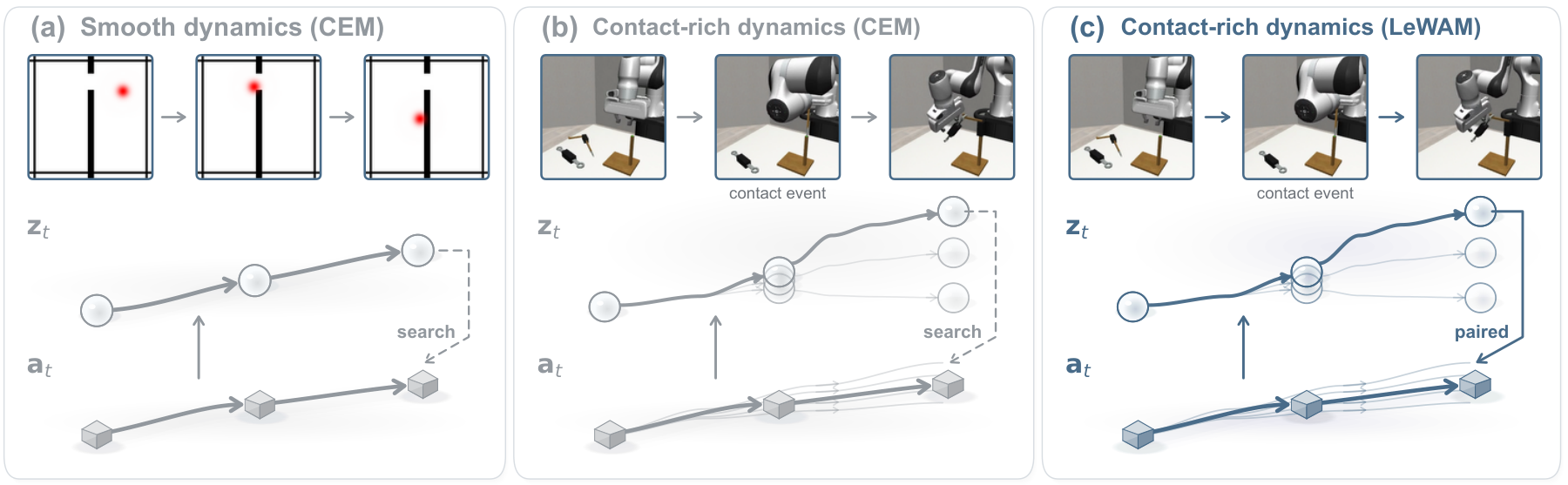
Contact transitions can make nearby actions produce different outcomes. A broad sampling prior may miss useful contacts, leaving little goal-cost signal for ranking plans. Learned action proposals improve the chance of starting in useful regions; predicted dynamics then evaluates and refines them.
The paper presents this explanation as a heuristic for difficult contact-rich search. A rigorous general verification remains future work (Pang et al., 2023) (Brudermüller et al., 2025).
Appendix F Author Contribution Statement
Minghao Fu initiated and led technical development and benchmarks. Tavis Siebert refined architecture, attention, planning, experiments, and released code. Eryk Halicki led the physical-robot system, data, and evaluation. Randall Balestriero initiated and supervised the project. All contributed to discussion, writing, and editing.