Overview
This is the complete 39-page arXiv v1 reading edition of SCOPE, including its mathematical and experimental appendices. The PDF is the figure-numbering reference: its omitted Maze2D Figure 8 is restored from the original PDF, and subsequent captions are relabeled accordingly. The original equations, tables, algorithm, references and project demonstrations remain available alongside the section notes.
At a glance
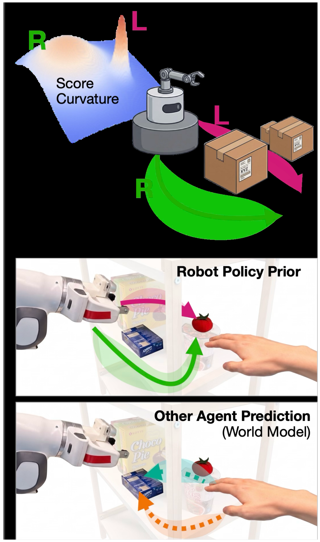
SCOPE turns a diffusion trajectory predictor into a Gaussian-mixture uncertainty interface for control. A lightweight head learns local score curvature during training, then predicts trajectory precision without repeatedly sampling the diffusion model at inference. The tubes describe local predictive variability, rather than epistemic confidence or a certified safe set. Experiments use simulated pedestrian forecasting/navigation, Maze2D planning and a Franka shelf task; the strongest hardware setting succeeds in 21 of 30 dynamic trials.
1 Introduction
A nominal trajectory omits how plausible nearby alternatives are, while estimating their spread with many diffusion samples can delay control. SCOPE adds structured local precision around explicitly indexed modes. It uses the resulting covariance either to predict moving obstacles or to shape sampling around a robot’s own plan. Mode weights represent distinct futures; the tube around each mode represents its local spread. These two kinds of uncertainty remain separate.
2 Preliminaries
The preliminaries connect diffusion denoising to the score of a trajectory density and introduce MPPI’s weighted rollout updates. MPPI evaluates sampled control sequences through dynamics and a running cost. Its exploration distribution determines which corrections it can discover with a limited rollout budget. SCOPE changes that interface rather than replacing collision checking with an unverified generated path.
3 Score-Curvature for Online Precision Estimation (SCOPE)
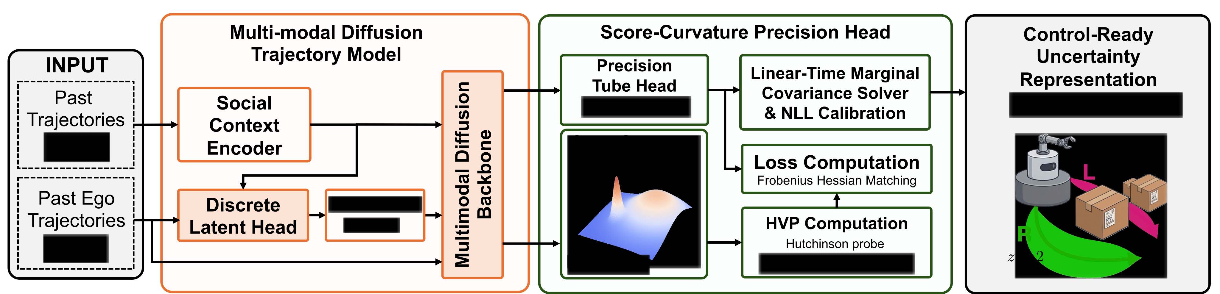
The method packages nominal trajectories, mode probabilities and positive-definite precision matrices into a mixture of Gaussian trajectory tubes. Its discrete multimodal backbone and precision head are trained in stages. Curvature supplies the head’s teacher signal; post-hoc likelihood scaling adjusts covariance magnitude. The approximation is local and depends on the backbone learning useful modes.
3.1 Control Interface Representation: From Local Tubes to Mixtures
Each mode supplies a mean trajectory and joint precision over the complete horizon. Inverting precision gives covariance blocks for individual future times. The mixture therefore separates between-mode alternatives from within-mode temporal dependence. It can wrap an ordinary diffusion prediction as well as explicit categorical modes, but fitting one Gaussian around an arbitrary sampled trajectory does not guarantee a globally faithful density.
Equation 1
| (1) |
3.2 Multimodal Diffusion Backbone
The backbone follows a categorical latent formulation with a context-conditioned mode prior and mode-conditioned diffusion decoder [13]. Its encoder posterior enables variational training, while the prior assigns mode probabilities at inference. A deterministic DDIM decode supplies one nominal trajectory per retained mode. The appendix adds mutual-information and usage regularizers to the displayed weighted ELBO; those additions are important to avoiding mode collapse.
Equations 2–3
| (2) |
| (3) |
3.3 Score-Curvature Precision Head
The head predicts a block-banded Cholesky factor plus a low-rank correction, producing positive-definite precision with local and long-range temporal couplings. Training matches its action on random probes to derivatives of a frozen diffusion score. Second derivatives are used during training, not repeatedly in the control loop. The teacher uses a small nonzero noise level in implementation; the terminal clean-density curvature is an approximation.
Equations 4–7
| (4) |
| (5) |
| (6) |
| (7) |
3.4 Using SCOPE in Downstream Control
As a forecaster, the tube becomes a Gaussian-mixture moving-obstacle model for MPPI’s collision-risk penalty. As a policy prior, a decoded path supplies warm starts/subgoals and its local covariance shapes exploration. For the single-integrator case, the next-waypoint state covariance is scaled by γ²/Δt², with γ below one. This is the paper’s chosen proposal design, rather than a general identity for arbitrary state/action dynamics.
4 Experiments
The experiments separately test uncertainty quality, policy-side rollout efficiency and forecasting inside closed-loop control. All quantitative results and implementation tables remain. Reported gains combine model quality with control behavior; they do not establish calibrated coverage, collision freedom or general transfer to raw visual observations.
4.1 SCOPE Precision Head Properties
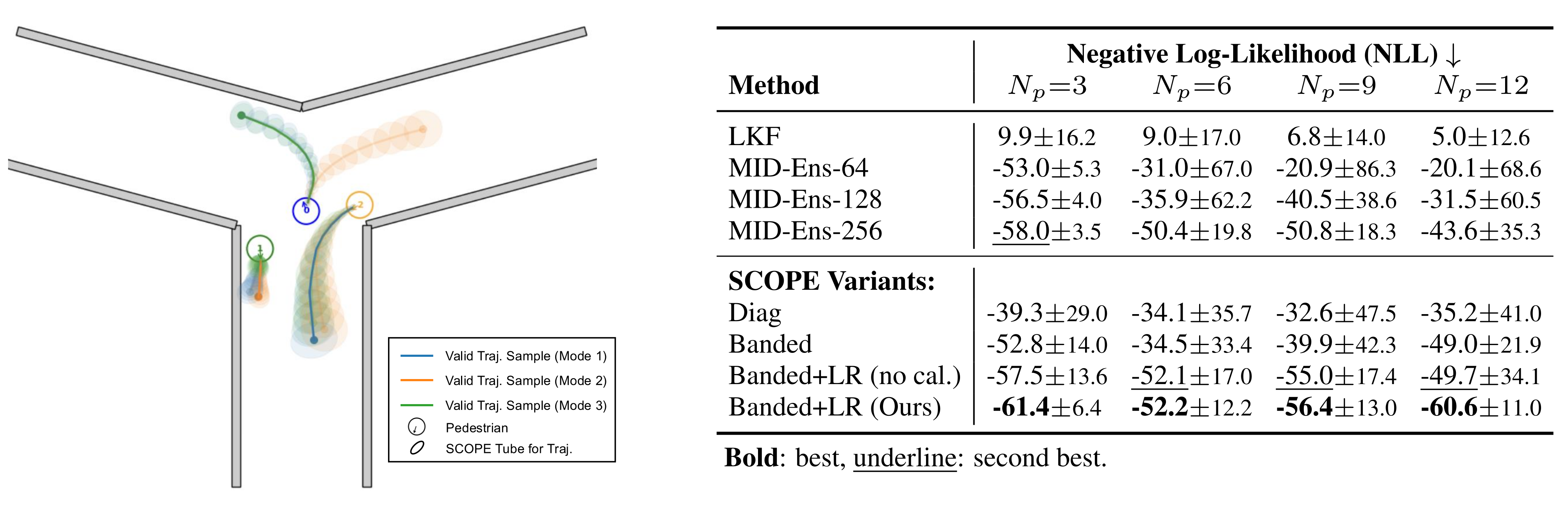
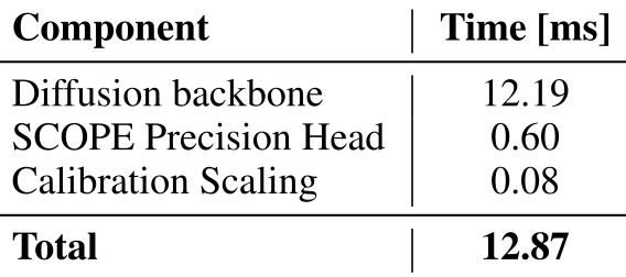
ORCA-generated junction data vary crowd size from three to twelve pedestrians. SCOPE’s calibrated banded-plus-low-rank head has the best reported trajectory NLL across all four densities, with −61.4, −52.2, −56.4 and −60.6. The shared backbone keeps its mean-trajectory accuracy unchanged across precision ablations. At three pedestrians, total inference is 12.87 ms on an A5000: 12.19 ms decoding, 0.60 ms precision and 0.08 ms calibration. Batched 256-sample ensembles take 91.779 ms, about 7.1 times as long.
4.2 Case Study 1: Maze2D Navigation
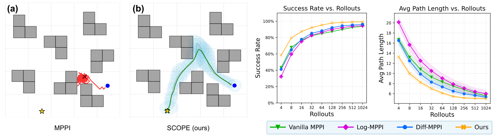
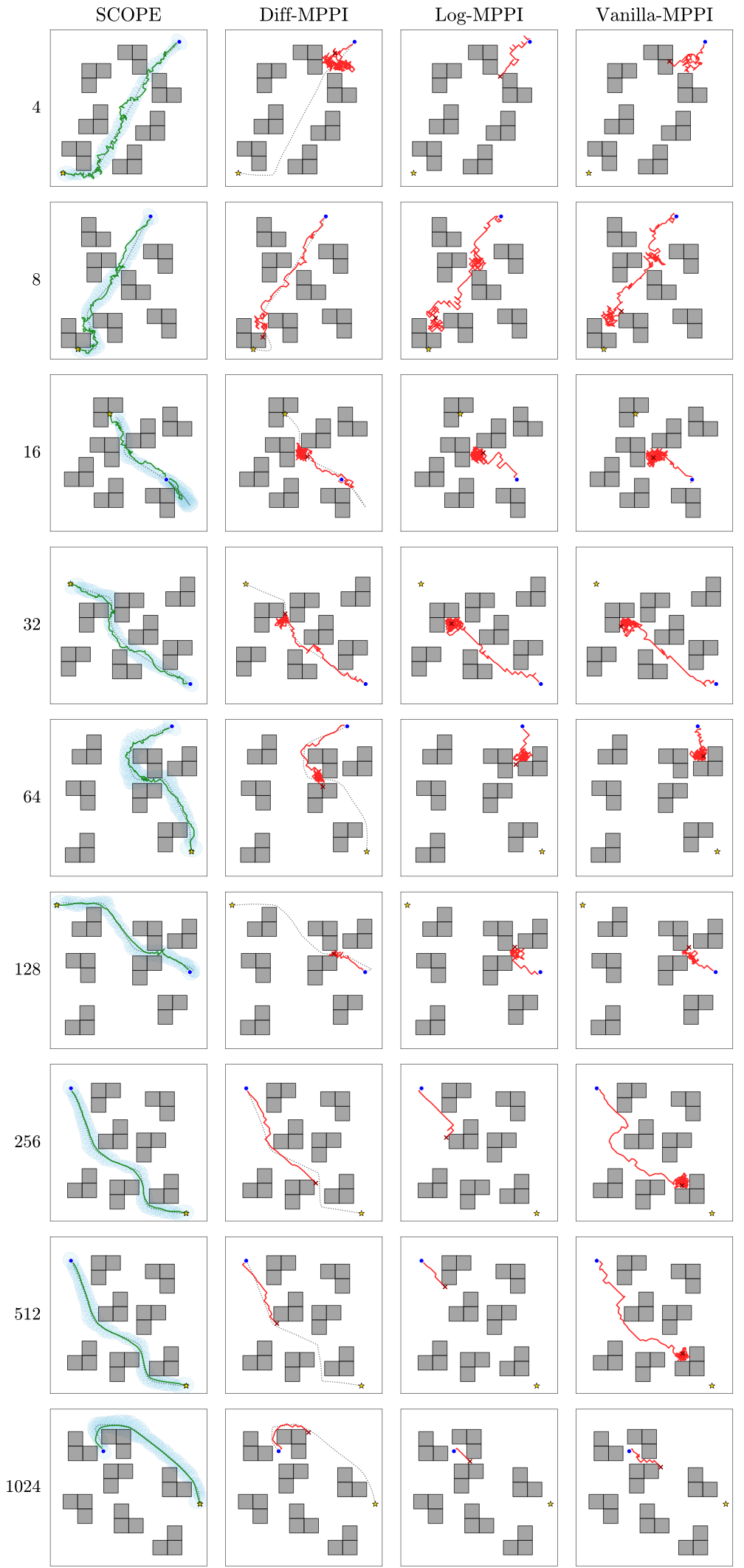
Maze2D contains unseen non-convex wall layouts that can trap short-horizon planners. Diff-MPPI and SCOPE share a diffusion path prior and subgoal tracking; SCOPE additionally changes the proposal covariance. Across the rollout sweep it reports better success and shorter paths. At 1,024 rollouts, success is 99.25% versus 96.35% for Diff-MPPI over 2,000 problems. The covariance is learned from feasible trajectories, while current geometric collision checks still evaluate rollouts.
4.3 Case Study 2: Y-Corridor Pedestrian Navigation
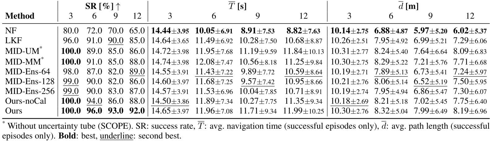
The junction controller consumes forecasts of online ORCA pedestrians. At three/six/nine/twelve pedestrians, calibrated SCOPE reaches 100/96/93/92% success in 100 episodes per density, versus 100/94/86/88% without calibration. Travel time and distance are reported only for successes, so their averages exclude failed episodes. The world model in this experiment is specifically a pedestrian-trajectory predictor, with latency-aware forecast reuse when computation cannot keep up.
Accessible table and original citation links
| SR [%] | [s] | [m] | ||||||||||
| Method | 3 | 6 | 9 | 12 | 3 | 6 | 9 | 12 | 3 | 6 | 9 | 12 |
| NF | 80.0 | 72.0 | 70.0 | 65.0 | 14.443.95 | 10.056.91 | 8.917.53 | 8.827.63 | 10.142.75 | 6.884.87 | 5.975.20 | 6.025.37 |
| LKF | 96.0 | 91.0 | 90.0 | 85.0 | 14.643.65 | 11.496.92 | 10.287.50 | 10.688.87 | 10.262.51 | 7.954.92 | 6.995.21 | 7.296.06 |
| MID-UM* | 100.0 | 89.0 | 85.0 | 86.0 | 14.723.98 | 11.957.68 | 11.199.59 | 11.8410.13 | 10.312.77 | 8.245.40 | 7.646.64 | 8.096.83 |
| MID-MM* | 100.0 | 91.0 | 85.0 | 88.0 | 14.743.98 | 12.087.47 | 10.568.18 | 11.259.84 | 10.302.75 | 8.295.22 | 7.215.76 | 7.716.68 |
| MID-Ens-64 | 98.0 | 87.0 | 82.0 | 89.0 | 14.553.91 | 11.437.22 | 9.897.72 | 10.598.64 | 10.192.71 | 7.895.13 | 6.735.41 | 7.245.97 |
| MID-Ens-128 | 99.0 | 90.0 | 82.0 | 86.0 | 14.603.97 | 11.687.25 | 9.577.42 | 10.958.66 | 10.212.76 | 8.065.14 | 6.525.19 | 7.505.95 |
| MID-Ens-256 | 99.0 | 90.0 | 83.0 | 87.0 | 14.573.91 | 11.536.96 | 10.047.85 | 10.718.91 | 10.192.74 | 7.954.94 | 6.865.47 | 7.306.07 |
| Ours-noCal | 100.0 | 94.0 | 86.0 | 88.0 | 14.503.86 | 11.897.34 | 10.277.75 | 11.359.34 | 10.182.69 | 8.215.18 | 7.025.45 | 7.756.40 |
| Ours | 100.0 | 96.0 | 93.0 | 92.0 | 14.653.97 | 11.967.08 | 11.719.34 | 11.9910.25 | 10.302.76 | 8.325.04 | 7.996.49 | 8.196.96 |
- *
4.4 Case Study 3: Real-Robot Manipulation
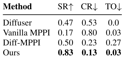
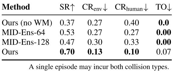
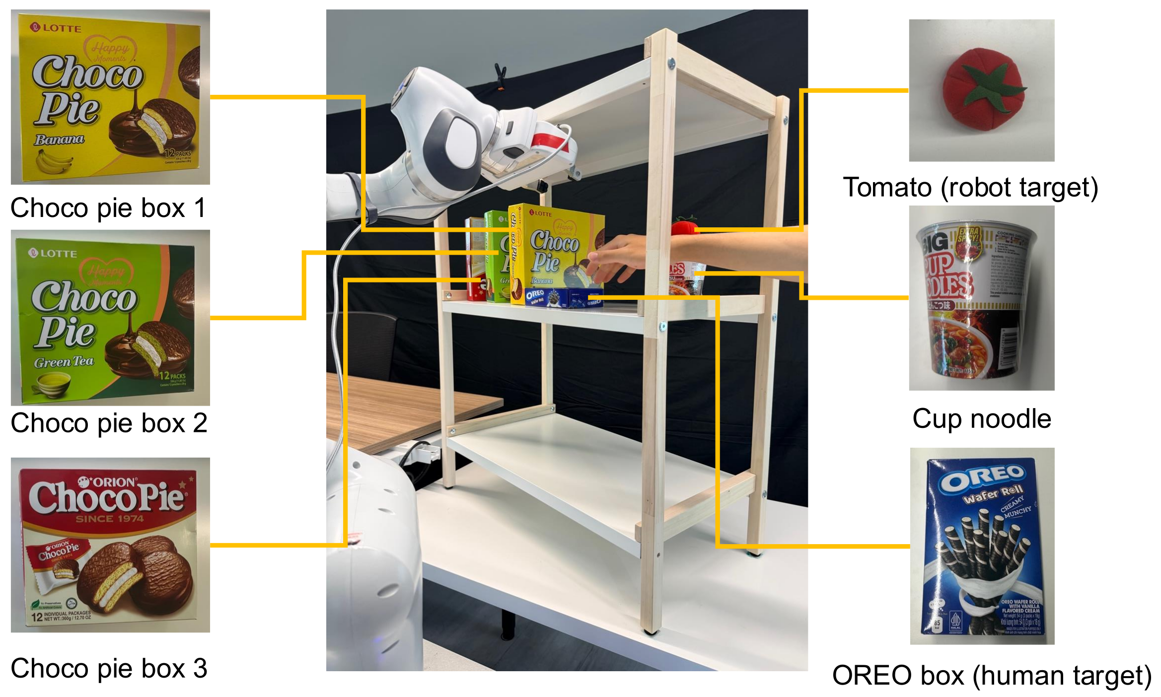
A Franka reaches into a shelf to move a tomato, with 30 trials per method and condition. Static SCOPE succeeds in 25/30 trials, versus 15/30 for Diff-MPPI, using 500 rollouts. Adding hand forecasting in the dynamic condition gives 21/30 successes, versus 11/30 without a hand world model and 16/30 with the 64-sample ensemble. Environment and hand collisions can occur in the same trial; their reported rates must not be summed as disjoint outcomes. Remaining failures include inaccurate occupancy and becoming trapped near the shelf.
5 Conclusion
The contribution is a compact bridge from diffusion predictions to controller queries: explicit modes, structured local uncertainty and inexpensive marginal covariance. The evidence supports useful low-dimensional forecasting and proposal design in the reported settings. It leaves broader observation modalities, out-of-distribution behavior and certified safety unresolved.
6 Limitations
The head inherits gaps in the learned diffusion distribution. Missing behaviors or poorly separated modes can make local tubes misleading. All experiments use relatively low-dimensional state and geometric context; applying the approach directly to images or point clouds is proposed future work. The controller retains nonzero collision rates.
Acknowledgments
The original acknowledgment names Singapore Ministry of Education support and French/Région Occitanie research funding. The first three authors contributed equally; Xue and Soh are corresponding authors.
Original project demonstrations
The primary SCOPE project page supplies 16 unchanged original videos with their original posters: an overview, four Maze2D comparisons, two crowd-navigation comparisons and nine shelf examples. Labels retain method and outcome, including collisions and a stuck baseline. They are selected demonstrations, rather than extra trials to add to reported success rates. The comparison scripts synchronize these existing videos and do not reveal additional video files.
Appendix A Related Works
The related-work appendix places SCOPE among trajectory diffusion, generative uncertainty and sampling-based robot control. Its distinction is the explicit precision interface distilled from local score curvature. The source’s full 47-entry bibliography remains linked.
A.1 Diffusion models for trajectory prediction.
Trajectory diffusion predicts pedestrian futures and also generates robot motion conditioned on goals or geometry. Prior systems use guidance, interaction conditioning and learned planning potentials [1] [2] [16]. Those capabilities alone do not supply per-mode precision or enforce downstream physical constraints. SCOPE adds an uncertainty representation around the learned futures.
A.2 Uncertainty quantification from generative trajectory models.
The target is aleatoric uncertainty over plausible futures. This differs from epistemic uncertainty about model parameters or unfamiliar inputs. Sampling-based covariance is expensive; reverse-process variances also need not equal clean-trajectory variability. Conformal prediction addresses a different question through calibrated coverage sets. SCOPE’s NLL fitting is not a conformal coverage guarantee.
A.3 Structured uncertainty for sampling-based control.
MPPI and related controllers combine sampled trajectories with geometric or probabilistic costs. Gaussian-process and structured prediction methods motivate temporal sparsity. SCOPE uses a banded-plus-low-rank precision to expose efficient covariance queries, while retaining explicit geometric evaluation and forecast-based risk penalties in the controller.
Appendix B Method Details
The supplement gives the local Gaussian argument, precision structure, theoretical query complexity, categorical diffusion training, calibration and probe/HVP identities. The complete mathematical displays are retained, including unnumbered definitions that explain the numbered equations.
B.1 Laplace’s Method
Laplace’s method approximates each mode-conditioned density locally with a Gaussian. The argument requires a smooth log density near a nondegenerate maximum, with positive-definite negative Hessian. A deterministic decoded trajectory is treated as a near-mode anchor; the appendix tests that assumption empirically rather than proving every anchor is a mode.
Equations 8–10
| (8) | ||||
| (9) | ||||
| (10) |
Local Taylor Expansion of the Log-Density.
At a genuine mode the score vanishes, removing the first-order Taylor term. The quadratic term then describes the local log-density shape. Away from a stationary point a linear term remains, so the nominal decode and the local quadratic center can differ. Keeping the expansion local matters when the complete mode-conditioned distribution is not exactly Gaussian.
Equations 11–13
| (11) |
| (12) | ||||
| (13) |
Recovering the Gaussian Approximation.
Negating the mode Hessian gives precision, and its inverse gives covariance. Exponentiating the second-order expansion recovers an approximate Gaussian after normalization. Positive semidefiniteness at a maximum is insufficient for an invertible covariance; the stated nondegeneracy assumption supplies strict positivity.
Equations 14–17
| (14) |
| (15) |
| (16) |
| (17) |
Anchor and curvature diagnostics.
The diagnostic uses 1,000 focal predictions from 20 held-out three-pedestrian episodes and the top three of six modes, giving 3,000 anchors. Raw symmetrized negative score Jacobians are positive definite at 2,843 anchors (94.8%). On that positive-definite subset, the weighted median quadratic-center shift is 1.33 cm. Querying learned covariance at the corrected center changes mixture NLL by 0.027. These observations support the approximation locally; they do not characterize away the remaining indefinite anchors.
B.2 Markov Sparsity in Trajectory Precision
For a Gaussian trajectory model, zero precision blocks encode conditional independence between times. A finite-order Markov assumption therefore motivates a block band. Learned diffusion trajectories can have longer-range dependence, so the low-rank term permits dense corrections beyond that band. This is a structured approximation rather than an assertion that all diffusion trajectories have exact Markov sparsity.
Equations 18–20
| (18) |
| (19) |
| (20) |
Empirical structure of teacher precision.
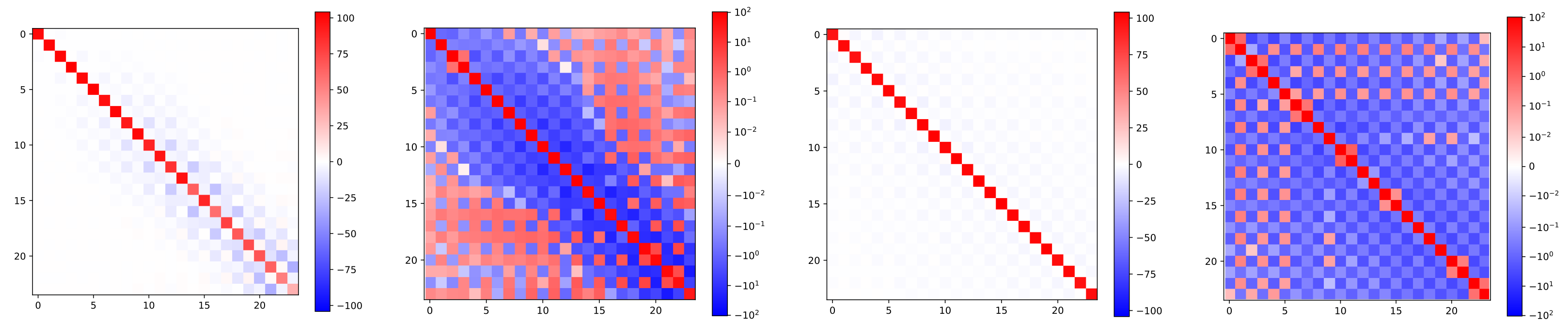
Figure 5 shows teacher precision for two representative trajectories at linear and symmetric-log scales. The plots exhibit diagonal dominance, near-diagonal structure and weaker off-band patterns. They motivate the chosen band-plus-low-rank parameterization; two examples alone do not establish that every teacher Hessian has that form or the chosen rank is sufficient.
B.3 Banded Cholesky Structure
A positive-definite block-banded matrix has a block-banded Cholesky factor with the same block bandwidth. Predicting that factor directly enforces the banded part’s positivity. For fixed block dimension and bandwidth, factorization scales linearly in horizon rather than cubically in the full flattened dimension. The low-rank addition handles remaining global coupling.
Equations
B.4 Inference Complexity Analysis
The derivation combines banded triangular solves, a Woodbury correction and selected inverse blocks. Its total theoretical cost is O(Tb²d³ + Tbd²r + Tdr² + r³), linear in horizon T when bandwidth b, state dimension d and rank r stay fixed. Crucially, the reported experiments use dense Cholesky and dense solves because pedestrian trajectories have d=2, T=12 and flattened dimension 24; the appendix reports this operation below 0.5 ms. The linear-time structured solver is a scalable implementation path, not the implementation benchmarked in those experiments.
Equations 21
| (21) |
B.5 Mixture-of-Diffusion Training Details
A discrete mode z and continuous noisy trajectory form the latent-variable model. Training introduces a posterior over modes, computes the diffusion variational term and enumerates the small mode set. The displayed weighted ELBO is augmented in implementation to encourage identifiable use of all modes.
Generative model.
The mode prior depends on context. Given a mode, reverse diffusion generates the clean trajectory from a Gaussian terminal noisy state. Conditioning combines context with the discrete mode, making global alternatives explicit before local uncertainty is attached.
Equation 22
| (22) |
Variational distribution.
The variational distribution factors into a learned posterior over modes and the fixed forward noising process given the recorded clean trajectory. Future ground truth enters the training posterior but is unavailable to the inference prior. Matching the two is part of the KL term.
Equation 23
| (23) |
ELBO derivation.
Applying the variational lower bound yields expected mode-conditioned diffusion likelihood minus the categorical posterior/prior KL. It is a lower-bound derivation before changing the KL weight and adding regularizers. The original multi-line equations retain the complete factorization and expectation structure.
Equations 24–27
| (24) |
| (25) | ||||
| (26) |
| (27) |
Diffusion VLB expansion.
The diffusion variational term expands into prior matching, reverse-step KL terms and reconstruction. Every term is conditioned on context and mode. The source notes the standard expansion without replacing it with a new uncertainty objective for the backbone.
Discrete enumeration.
Because there are few categorical modes, the posterior expectation is summed exactly over z. This avoids a sampled categorical approximation for that part of training. It does not eliminate diffusion noise/time sampling in the conditional likelihood training.
Equation 28
| (28) |
Training loss.
The minimized base objective is posterior-weighted negative diffusion likelihood plus β times the mode KL. The final recipe adds a posterior mutual-information reward with coefficient 0.12 and a batch-marginal usage penalty decaying from 0.20 to 0.02. The latter penalizes deviation from uniform batch usage. These terms encourage diverse mode use, without proving semantic independence or perfect mode separation.
Equation 29
| (29) |
B.6 Multimodal Backbone Diagnostics
Backbone diagnostics examine mode usage, sensitivity to mode count and the single-basin assumption within each mode. They use held-out junction contexts and distribution-shape tests. The results support the representation empirically within this setting; the diagnostic scope is narrower than a general unimodality theorem.
Mode usage.
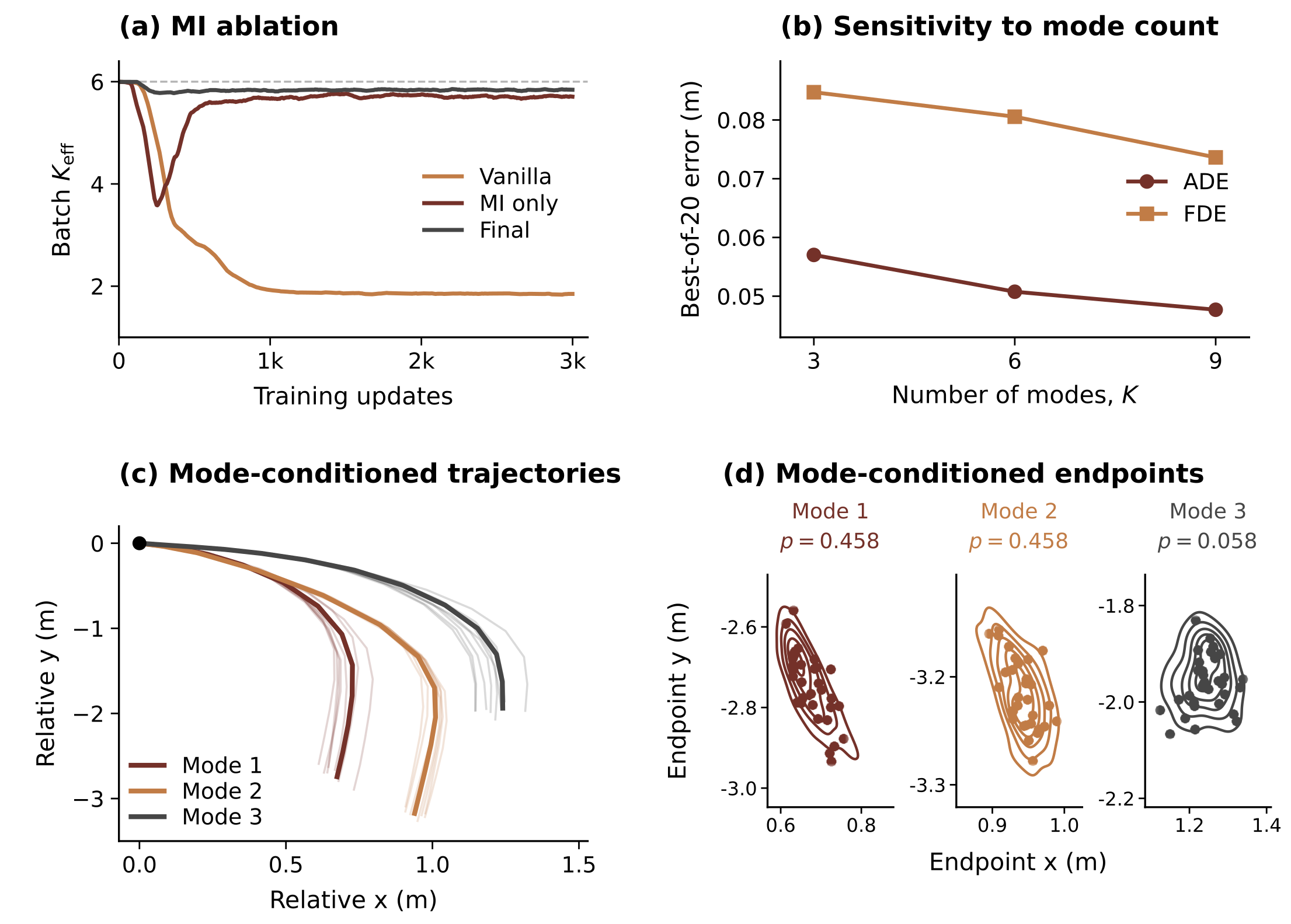
Without mutual-information or usage regularization, only two of six modes are active and effective count is 1.84 on 1,000 held-out contexts. Mutual-information training activates all six with effective count 5.79; the final recipe reaches 5.90. Activity means highest posterior probability in at least 1% of contexts. Effective count is derived from aggregate posterior perplexity, not a per-context count of six equally likely futures.
Sensitivity to mode count.
Matched K=3/6/9 training uses 1,017 held-out contexts and best-of-20 displacement error. ADE/FDE improve from 0.057/0.085 m at K=3 to 0.048/0.074 m at K=9. These oracle-style sample metrics do not measure whether an online controller can select the best sample or whether its probability calibration improves equally.
Mode-conditioned unimodality.
For 200 held-out contexts, retained modes cover at least 95% prior mass and supply 128 trajectories each. Endpoint and trajectory-PCA KDE checks search for secondary basins across bandwidth changes and bootstrap resampling. Passing conditionals account for 93.34% of evaluated probability mass, with a context-bootstrap 95% interval of 89.94–96.40%. The residual mass and density-test limitations remain; the method does not assume a universally exact single Gaussian.
B.7 Trajectory-Level NLL Calibration
A disjoint 10% calibration split fits per-horizon covariance scales by full-trajectory mixture NLL; 70% trains the models and 20% is test data. Mode weights, means and raw covariance predictions are frozen. The objective improves likelihood scale without explicitly optimizing a coverage target or correcting mode probabilities.
Per-horizon inflation factors.
Each learned scale is exp(sₜ), ensuring positivity. Although called an inflation factor, it can exceed one or fall below one, widening or shrinking the covariance. Scale one leaves that horizon unchanged. There is no τ≥1 restriction in the displayed parameterization.
Equation 30
| (30) |
Symmetric scaling of the full covariance.
The complete covariance is scaled symmetrically as DΣD, with sqrt(τₜ) repeated across spatial coordinates. This preserves symmetry, positive definiteness and correlation coefficients. Cross-time blocks scale by sqrt(τₛτₜ), retaining a coherent joint covariance instead of editing only marginal diagonal blocks.
Equations 31–32
| (31) |
| (32) |
Trajectory-level GMM log-likelihood.
The Gaussian likelihood is evaluated over the flattened complete trajectory. Log-sum-exp over modes occurs once for the whole horizon. Summing separate per-time mixture likelihoods would implicitly allow modes to switch between timesteps and discard the modeled joint dependence. The determinant and quadratic-form identities exploit D while retaining a Cholesky factor of the original covariance.
Equations 33–36
| (33) |
| (34) | ||||
| (35) |
| (36) |
Calibration objective.
The calibration loss is average joint trajectory NLL plus an ℓ₂ penalty on log scales. Regularization shrinks scales toward one, limiting extreme covariance adjustments on the calibration split. Only the T scalar log scales receive gradients; the backbone, precision head and mixture probabilities remain fixed.
Equation 37
| (37) |
Optimisation and data split.
Adam fits the log scales for a fixed iteration count on the separate calibration predictions. All reported metrics use the disjoint test partition. The resulting rescaling is inexpensive at inference, but held-out fitting alone does not provide distribution-free guarantees under future shift.
B.8 Hutchinson Trace Estimator: From Matrix Matching to Probe Matching
Direct dense Hessian supervision would be costly. Hutchinson probe matching replaces the squared matrix error with an expected squared error in how the two matrices act on isotropic random vectors. The equality holds in expectation over probes, not as an exact equality for each finite sampled training batch.
Equation 38
| (38) |
Hutchinson identity.
For error matrix M and E[uuᵀ]=I, E‖Mu‖² equals tr(MᵀM)=‖M‖²F. Gaussian probes satisfy the isotropy condition. This explains the matrix-matching target without materializing the teacher Hessian; finite-probe variance and approximation of the teacher score remain separate issues.
Equations 39–41
| (39) |
| (40) |
| (41) |
B.9 HVP Identity: Efficient Teacher Signal
The score derivative supplies the teacher’s response to a probe. Automatic differentiation of a scalar score/probe inner product returns a vector without constructing the full Hessian. The score is learned and evaluated at a small nonzero terminal noise level, so the practical target approximates clean-density curvature.
Score–curvature relationship.
For an exact conservative score, its Jacobian is the log-density Hessian. The negative Hessian is the local precision teacher. The implementation substitutes a small nonzero diffusion noise level for ideal time zero. A learned score is not guaranteed exactly conservative or positive definite at every queried anchor.
Equations 42–43
| (42) |
| (43) |
HVP derivation.
Differentiating s(y)ᵀu with respect to y yields the transposed score-Jacobian response, equal to the Hessian response for a true gradient score. One backward pass produces the desired vector under that assumption. The source’s curvature diagnostics symmetrize raw Jacobians; this distinction matters when interpreting the learned teacher as a mathematical precision.
Equation 44
| (44) |
Final training loss.
The head’s precision/probe product is matched to the negative gradient of the frozen score/probe scalar. The backbone stays frozen while the head learns. Hutchinson supplies the expected Frobenius interpretation and autodiff supplies the teacher response. The positive-definite student structure can approximate the signal without making every raw teacher matrix positive definite.
Equation 45
| (45) |
Appendix C MPPI Control Details
The control appendix retains all costs, the collision-probability derivation and the five-step tube-to-proposal algorithm. World-model risk and policy-side exploration use different parts of the Gaussian representation. Neither generated trajectories nor likelihood calibration replace closed-loop geometric checks.
C.1 MPPI Cost Function Design
Junction MPPI sums weighted goal distance, soft wall avoidance and Gaussian-mixture risk costs across the planning horizon. It rolls deterministic robot dynamics for candidate action sequences. A smooth penalty encourages acceptable predicted risk; feasibility is not enforced as a hard optimization constraint.
Equation 46
| (46) |
C.1.1 Goal-Reaching Cost
The goal term sums Euclidean robot-to-goal distance at every horizon step. It guides intermediate states rather than evaluating only the terminal point. This junction cost differs from Maze2D’s squared-distance and large binary wall penalty, whose separate settings remain in the experimental appendix.
Equation 47
| (47) |
C.1.2 Wall-Avoidance Cost
A geometry module returns wall clearance. Softplus penalizes falling below a comfortable clearance margin, with a width parameter smoothing the transition. Its tail decays outside the margin but remains positive; it is a soft barrier rather than an impenetrable geometric constraint.
Equation 48
| (48) |
C.1.3 GMM Chance-Constrained Collision Cost
For each time, a union bound sums collision probabilities across agents, and each mode’s disk-collision event is bounded by a separating half-space Gaussian probability. The weighted sum can exceed one and is used as a conservative risk surrogate. Squared softplus penalizes exceeding budget δ. If the modeled bound is below δ then the model’s per-time collision probability is bounded, but MPPI’s finite-weight soft objective need not satisfy that condition. The statement is neither a whole-horizon probability guarantee nor a calibrated real-world safety guarantee.
Equations 49–55
| (49) |
| (50) |
| (51) |
| (52) |
| (53) |
| (54) |
| (55) |
C.2 Derivation of the Collision Probability Upper Bound (one agent)
The collision disk lies inside the half-space perpendicular to the mean separation direction. Projecting each Gaussian onto that direction gives a scalar normal CDF bound; mode probabilities then combine the bounds. The derivation is valid for the assumed Gaussian-mixture marginal and disk geometry, including correlated agents through the union bound without requiring their independence. The displayed normalized direction is undefined at zero mean separation unless an implementation adds a convention; the source does not specify one here.
Equations 56–70
| (56) |
| (57) |
| (58) |
| (59) |
| (60) |
| (61) |
| (62) |
| (63) | ||||
| (64) | ||||
| (65) |
| (66) | ||||
| (67) | ||||
| (68) | ||||
| (69) | ||||
| (70) |
C.3 SCOPE Algorithm Details
Policy-side control starts from a single global path, follows it with forward-progress subgoals and caches a time-varying proposal covariance. These details are important: SCOPE’s benefit is not evaluated as covariance attached to a controller with no path initialization or tracking logic.
C.3.1 Notation and overview
The path is resampled and cumulative arclength computed once per episode. Single-integrator dynamics relate 2D velocity controls to successive states. The precision head is queried once on the selected path, rather than at every local rollout state.
C.3.2 Nominal MPPI control sequence
The initial MPPI nominal sequence follows velocities along the diffusion path. Later control steps shift the current nominal forward and refine it through weighted sampled perturbations. This preserves global guidance while allowing local deviation from the generated reference.
Warm-start from diffusion path.
Initial actions are adjacent waypoint differences divided by Δt, with the final action copied from its predecessor. The first rollout batch is therefore centered on a learned path rather than zero/random controls. Diff-MPPI shares the global-path reference in the comparison.
Equation 71
| (71) |
Receding-horizon refinement.
At each receding-horizon step, Gaussian perturbations use the cached tube-shaped covariance and the updated nominal. MPPI evaluates goal/subgoal tracking and wall penalties, then applies the weighted action correction. The generated reference remains a soft guide rather than a hard executed trajectory.
C.3.3 Subgoal selection
Subgoals use a monotone nearest-path index followed by arclength lookahead. This prevents jumping backward when a path crosses itself and gives the local controller a forward target. It also constrains recovery: a short-horizon controller can still become stuck when reaching safety requires backing out.
Monotone nearest index.
The nearest waypoint search is limited to a forward window of 20 waypoints from the previous progress index. This enforces nondecreasing path progress. It is an execution heuristic rather than a proof of global progress or successful escape from every concave obstacle configuration.
Equation 72
| (72) |
Arclength-based lookahead.
The next target is the first waypoint at least the chosen arclength ahead. Near the path end, or when less path remains than that lookahead, the target switches to the true goal. Maze2D uses a 0.4-unit lookahead.
Equation 73
| (73) |
C.3.4 Precision tubes for exploration covariance
State marginals are rescaled back to configuration space and used to shape action exploration. Covariance windows and sampling factors are cached once per episode. Although the model learns full temporal precision, the displayed proposal mapping uses next-waypoint marginal covariance; the controller does not directly sample the complete learned joint trajectory Gaussian.
State-to-action mapping.
The rule Σᵘᵢ=(γ²/Δt²)Σˣᵢ₊₁ narrows the tube with γ below one and converts units for single-integrator velocity controls. Algorithm 1 separates episode-level covariance/factor preparation from per-step window retrieval and sampling. The original PDF’s five numbered steps and unnumbered headings are preserved in the native layout.
Equations 74–75
| (74) |
| (75) |
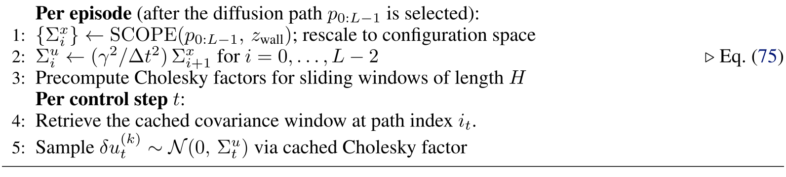
Original selectable algorithm
Appendix D Experiment Details
The experiment appendix supplies the complete accuracy, configuration, timing and navigation tables. Junction forecasting and closed-loop control reuse the same checkpoints; Maze2D trains an independent prior/head. The hardware system adapts the policy-side model to eight-dimensional joint/gripper trajectories and adds hand prediction for the dynamic condition.
D.1 Shared Y-Corridor Setup
Trajectron++ history/social encoders provide a 256-dimensional context. Six discrete modes condition a 100-step diffusion model, decoded in five DDIM steps. The frozen backbone supplies context/mode features to the precision head, followed by trajectory-level calibration. Forecasting and navigation share the dedicated 70/20/10 train/test/calibration split.
D.2 Forecaster Quality on Y-Corridor
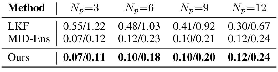
Four ORCA datasets use Δt=0.4 s, eight observed steps and twelve predicted steps. Evaluation caps scene contributions and collects up to 1,000 test pairs per density; sequence means are then summarized across scenes. MID ensembles fit three full-covariance components to 64/128/256 samples. SCOPE retains the three most probable of six modes, renormalizes their weights, decodes once per retained mode and predicts covariance directly. Mode weights themselves are not calibrated. Best-of-mean ADE and FDE select minima separately.
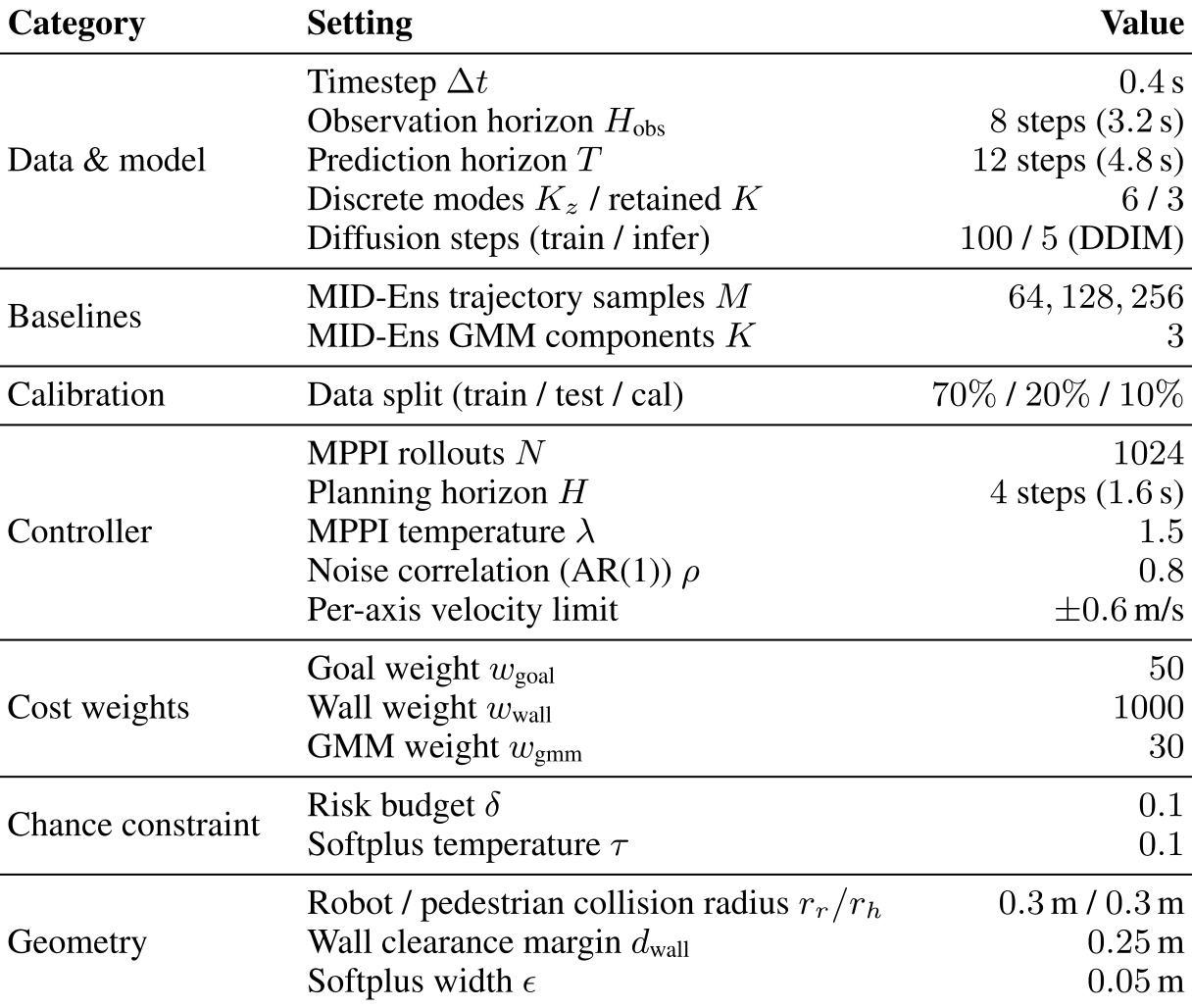
Accessible table and original citation links
| Category | Setting | Value |
| Data & model | Timestep | s |
| Observation horizon | steps ( s) | |
| Prediction horizon | steps ( s) | |
| Discrete modes / retained | / | |
| Diffusion steps (train / infer) | / (DDIM) | |
| Baselines | MID-Ens trajectory samples | |
| MID-Ens GMM components | ||
| Calibration | Data split (train / test / cal) | / / |
| Controller | MPPI rollouts | |
| Planning horizon | steps ( s) | |
| MPPI temperature | ||
| Noise correlation (AR(1)) | ||
| Per-axis velocity limit | m/s | |
| Cost weights | Goal weight | |
| Wall weight | ||
| GMM weight | ||
| Chance constraint | Risk budget | |
| Softplus temperature | ||
| Geometry | Robot / pedestrian collision radius | m / m |
| Wall clearance margin | m | |
| Softplus width | m |
D.3 Inference Time Comparison
All ensemble diffusion calls are fully batched on an A5000. Total times are 26.581/47.527/91.779 ms for 64/128/256 samples, versus 12.87 ms for SCOPE; increased crowd size adds latency, with a reported roughly 200 ms at nine pedestrians and 256 samples. One decode per retained mode is batched, rather than one new Monte Carlo ensemble. During delayed updates pedestrians keep moving and the controller interpolates the previous forecast. Figure 7’s marginal confidence-ellipse coverage improves after NLL scaling, but the source explicitly calls it a diagnostic without formal coverage guarantees.

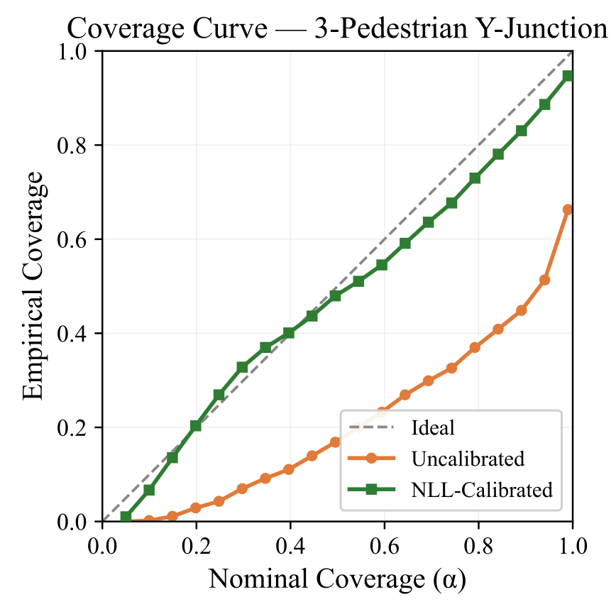
D.4 Maze2D MPPI Sample-Efficiency
Maze2D uses a 5×5 workspace, seven rectangular walls, single-integrator dynamics at 0.1 s and a 0.01 robot radius. A shared prior trains on about 2.34 million trajectories from 3,000 mazes. Evaluation has 100 held-out mazes with 20 fixed start/goal pairs each, repeated across nine rollout budgets from four to 1,024. Each method uses one decoded style/path, with no best-of-candidate selection. Success requires reaching within 0.3 of the goal by 200 steps and remaining collision-free at waypoints plus 0.05-spaced interpolants. The head’s trace-variation regularizer prevents a reported nearly isotropic collapse in preliminary training.
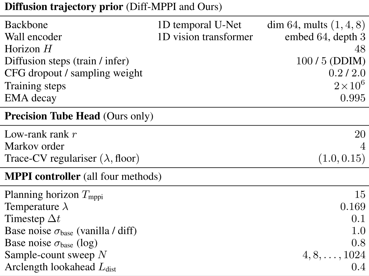
Accessible table and original citation links
| Diffusion trajectory prior (Diff-MPPI and Ours) | ||
| Backbone | 1D temporal U-Net | dim , mults |
| Wall encoder | 1D vision transformer | embed , depth |
| Horizon | ||
| Diffusion steps (train / infer) | / (DDIM) | |
| CFG dropout / sampling weight | / | |
| Training steps | ||
| EMA decay | ||
| Precision Tube Head (Ours only) | ||
| Low-rank rank | ||
| Markov order | ||
| Trace-CV regulariser | ||
| MPPI controller (all four methods) | ||
| Planning horizon | ||
| Temperature | ||
| Timestep | ||
| Base noise (vanilla / diff) | ||
| Base noise (log) | ||
| Sample-count sweep | ||
| Arclength lookahead | ||
D.4.1 Maze2D Navigation Results
At 1,024 rollouts SCOPE reports 99.25% success, 0.65% collision, 99.90% goal reaching and path length 4.996±0.763 m. Diff-MPPI reports 96.35%, 2.60%, 98.75% and 5.328±1.601 m. Goal reaching alone includes colliding executions; success excludes them. The 0.65% collision rate ties Log-MPPI rather than uniquely winning that metric. Restored Figure 8 shows selected challenging cases at each rollout budget; they illustrate behavior rather than provide a second unbiased test set.
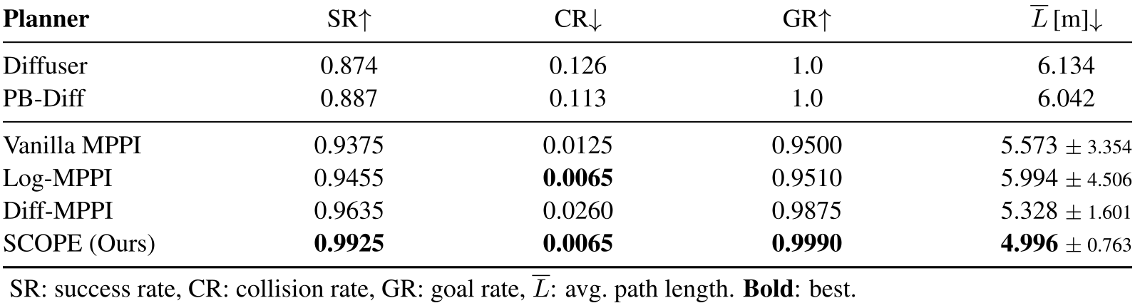
Accessible table and original citation links
D.5 Y-Corridor Closed-Loop Navigation
The online junction simulator runs 100 episodes for each of four crowd densities. Every forecaster passes the same mean/covariance interface to a controller with 1,024 rollouts and four-step horizon. All diffusion decoding is batched; NF/LKF, unimodal/multimodal MID, ensembles and calibration ablation differ in forecasting. Success excludes collision and timeout, while distance/time include only successful trials. Source results do not supply independent training-seed confidence intervals for those success rates.
D.6 Direct NLL Training of the Precision Head
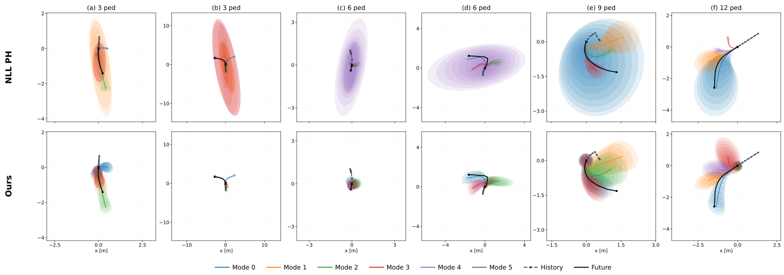
A direct-NLL precision head shares architecture, frozen backbone and means with SCOPE. Its navigation success is 100/91/84/81%, versus 100/96/93/92% for curvature training as crowd density rises. The proposed explanation is that NLL can widen covariance to absorb fixed-mean error, increasing the controller’s risk cost outside a collision radius. Figure 9 contains selected examples, so this mechanism is an interpretation consistent with the experiment rather than a universal causal proof against likelihood training.

D.7 Real-Robot Experiments
The complete hardware appendix retains calibrated geometry, task/trial definitions, model adaptation, mode selection and execution details. Static and dynamic tests share the shelf task; dynamic trials add a reaching hand. The demonstrations are selected qualitative examples alongside the full 30-trial tables.
D.7.1 Environment and Hardware
The platform is a seven-joint Franka Panda with Franka Hand gripper. Prebuilt cuboids represent the shelf and movable boxes, with poses aligned using wrist RealSense point clouds before execution. Two RGB webcams observe the hand in dynamic trials. Control uses an RTX 5090 workstation, rather than deriving the complete obstacle scene from raw images online.
D.7.2 Task Setup and Evaluation Protocol
Each method receives 30 trials per condition, with boxes repositioned near the tomato. A collision-free run that has not completed by 120 s is a timeout. Dynamic environment and hand collisions are counted separately and can co-occur. Front and tighter side approach modes vary in room for correction; the reported trials do not establish safety over arbitrary shelf geometry or unrestricted human motion.

D.7.3 Controller and System Implementation
The system calibrates cuboid poses, generates joint-space candidate modes and uses tube shape both for mode selection and MPPI exploration. Hand forecasts add moving collision primitives. The appendix gives the 50 Hz controller rate but does not equate that with continuously regenerating the full diffusion path at 50 Hz.
Static scene calibration.
Point-cloud calibration establishes SE(3) poses for the fixed collision primitives before each trial. The controller keeps those primitives fixed during execution. Updating their poses when layouts change is part of the experimental setup, not an evaluated open-world perception capability.
Diffusion and SCOPE.
The robot diffusion/head predicts trajectories in eight dimensions: seven joint coordinates and one gripper coordinate. Scene conditioning becomes calibrated cuboid poses instead of a 2D wall layout. Joint-space tube estimates support the selected approach, without representing all possible environment or perception uncertainty.
Mode selection.
Of two approach modes, the system selects the one maximizing the minimum covariance eigenvalue encountered along its normalized trajectory. This favors flexibility at the tightest point. It is covariance-based mode selection, not simply choosing the most probable mode or proving the selected path has maximum physical clearance.
Equations
Tube-informed MPPI controller.
MPPI tracks a local point ahead on the selected smooth joint-space reference. Tube shape adjusts perturbations, while calibrated collision geometry checks rollouts. A constraint-aware score strongly downweights unsafe rollouts, inspired by COSMIK-MPPI, instead of relying solely on additive penalties. The soft reference permits deviations but finite-horizon recovery can still fail.
Human hand tracking and prediction.
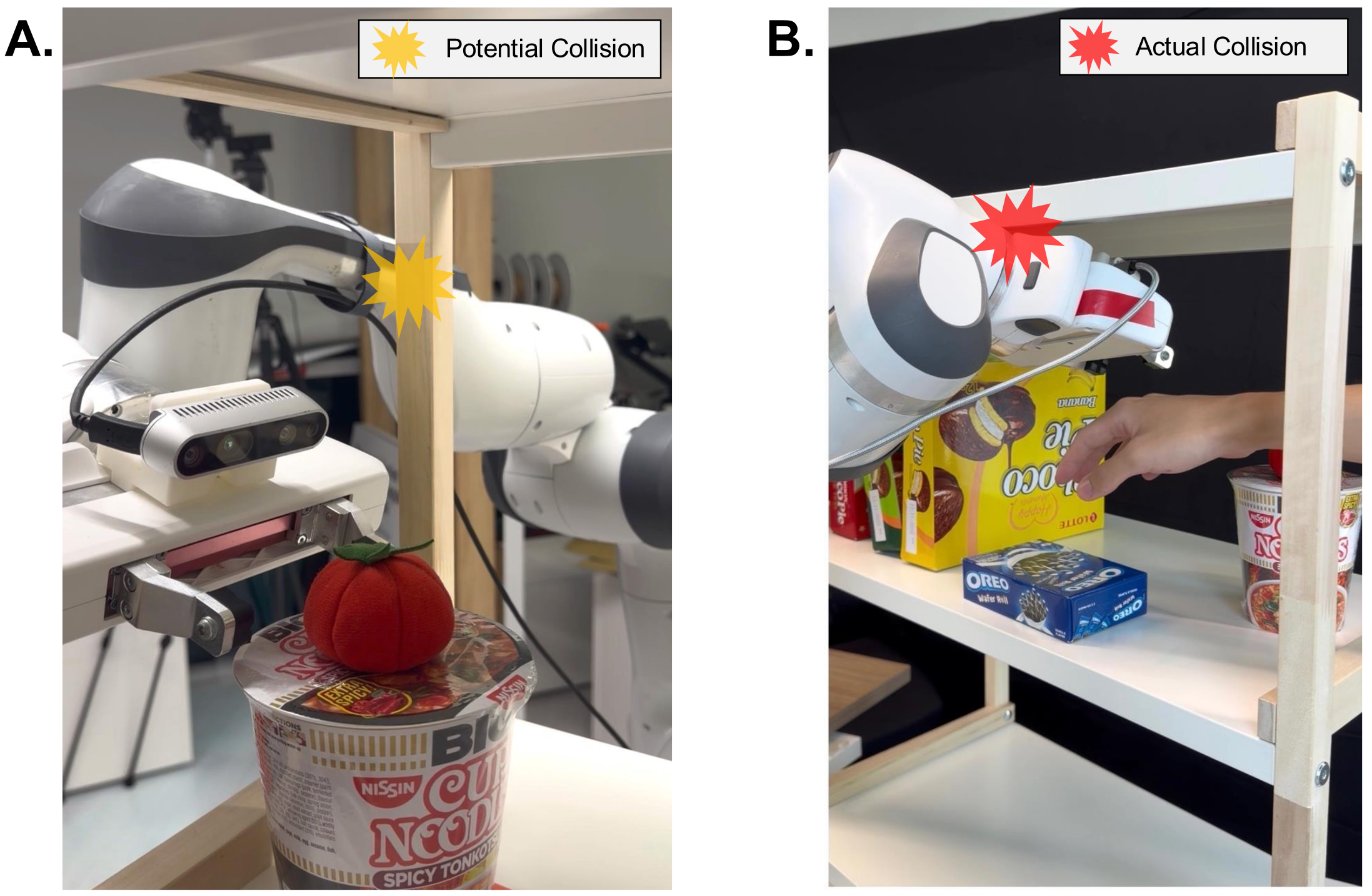
Two-camera markerless tracking supplies hand observations to a diffusion predictor. SCOPE augments its future trajectory with uncertainty, converted to time-varying collision primitives. The human model covers the hand relevant to this tabletop task, rather than the whole body or all possible human behavior.
Execution.
At trial start the system calibrates geometry, measures robot state, predicts candidate modes and chooses one. The 50 Hz MPPI loop then projects current state onto a forward-progress index and follows a lookahead reference, balancing collision, joint-limit and control costs. The robot is not committed to executing every diffusion waypoint open-loop.
D.7.4 Real-Robot Case Studies
Figure 12 illustrates a static timeout when a tight side approach leaves insufficient room to back out, and a dynamic no-world-model failure where late hand avoidance drives the arm into the shelf. Full hand prediction can prompt earlier yielding before entering that constrained region. These cases explain observed failure modes; full SCOPE still records static and dynamic collisions.