Overview
A rolling action buffer lets a flow-based VLA refine future actions across observations while retaining a long horizon. This edition retains all original figures, equations, tables, failure examples and ablations. Project page.
At a glance
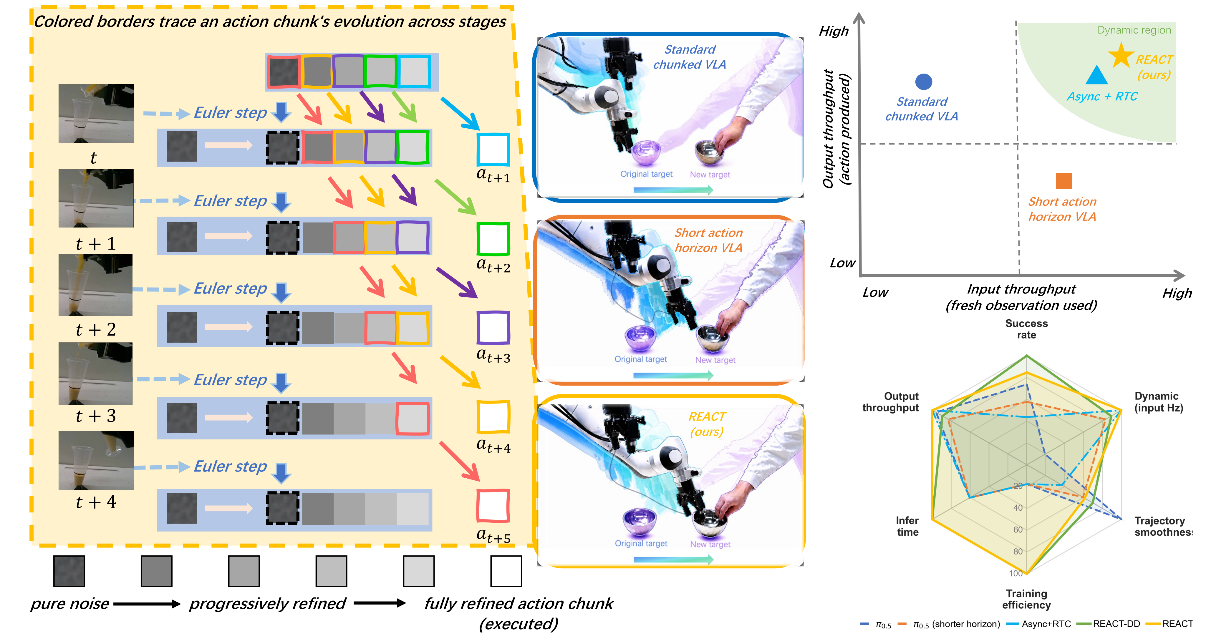
REACT combines staggered flow times, persistent future-action blocks, schedule-matched training and asynchronous deployment. It improves the tested success–reactivity trade-off over independently replanned and Async+RTC baselines. Full REACT streams actions faster, while its synchronous variant achieves slightly higher general-task success. Evidence covers one VLA backbone, seven simulation tasks and two real bimanual platforms; it does not establish training-seed robustness or seamless switching between schedules.
1 Introduction
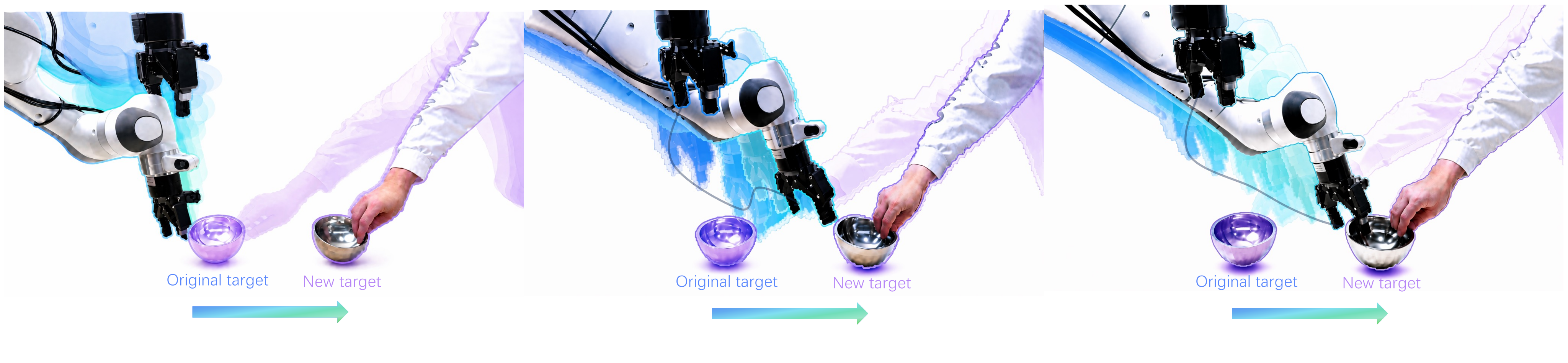
Long action chunks preserve coherent motion but delay new visual feedback; short replanning intervals can repeatedly restart an incomplete contact skill or switch between plausible action modes. REACT evaluates both fresh observations consumed per second and executable actions produced per second. Instead of regenerating a chunk, it maintains one long buffer whose future blocks are gradually denoised under newer observations. A separate scheduler overlaps perception and control; matched staircase training supervises the deployed time-position combinations.
2 Related Work
The method builds on chunked imitation and flow-based VLAs, including π0.5. Acceleration reduces inference cost, asynchronous execution hides it, and training-time RTC conditions new chunks on committed actions; these do not necessarily make their conditioning fresh at execution. Rolling diffusion and Diffusion Forcing provide related staggered-generation ideas. REACT adapts them to a VLM/action-expert stack, where perception and action generation can be separately scheduled. The paper compares particular implementations, not every asynchronous or rolling policy.
3 Methodology
Three components work together: rolling flow refinement, a scheduler that decouples observation processing from action dispatch, and training with the same staircase of flow times.
3.1 Rolling Denoising for Flow-Based VLAs
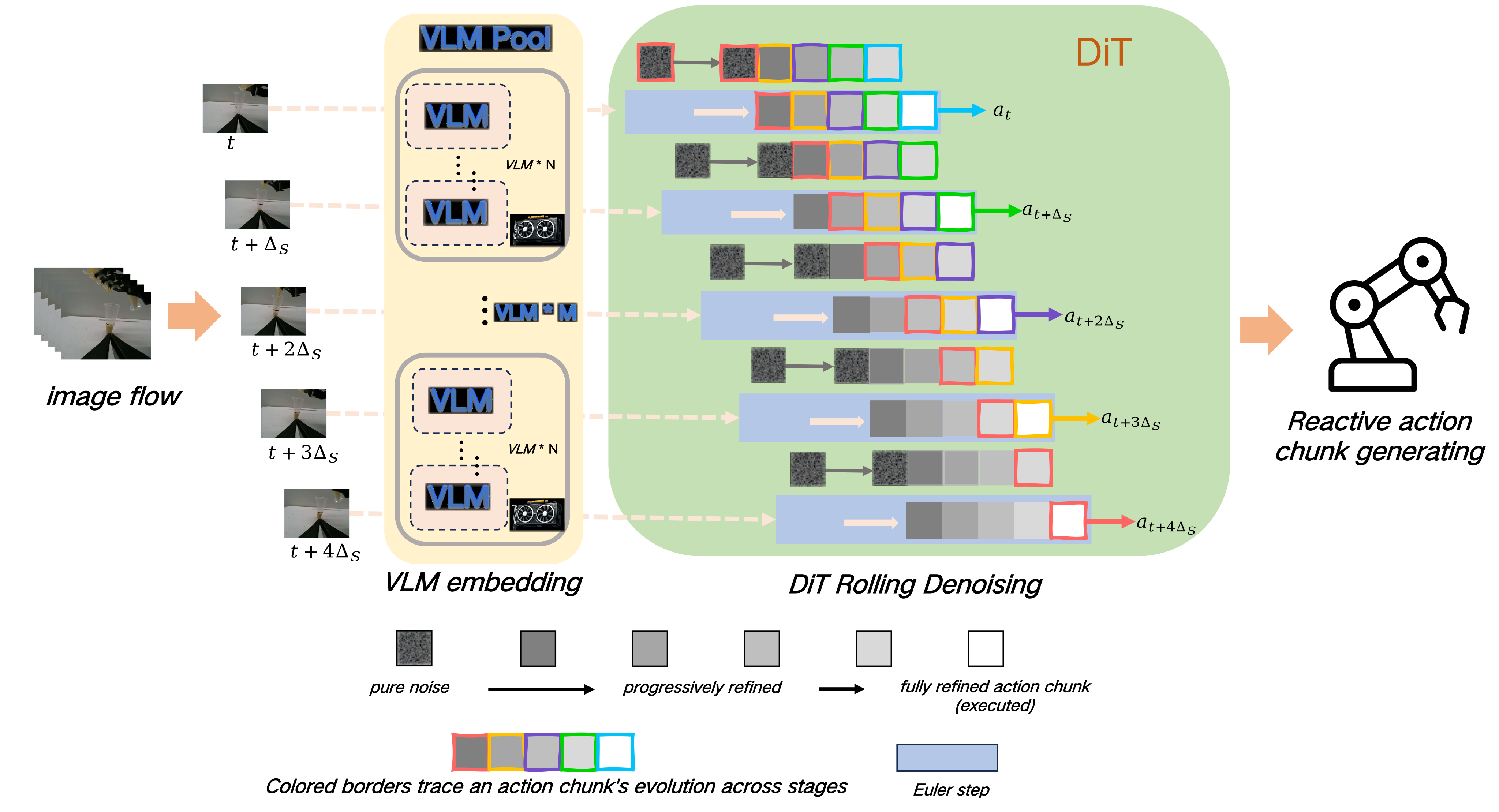
The flow-matching convention is noise at τ=1 and clean action at τ=0. Partition H=KS actions into K blocks; block k starts each update at τ=(k+1)/K. One full-buffer action-expert pass followed by an Euler step of size 1/K makes the front block executable. Emit its S actions, shift the partially refined remainder left, and append fresh Gaussian tail noise. A block therefore receives K refinements before execution, usually under successive observations. The main setting H=50, K=5, S=10 keeps future context while avoiding independent suffix regeneration. Its continuity is empirically supported, not a formal guarantee that modes cannot change.
Equations 1–3
| (1) |
| (2) |
| (3) |
3.2 Dual Decoupling for High-Throughput Deployment
Dual Decoupling separates sensing, VLM encoding, action-expert denoising and execution without changing the trained REACT weights. Select one frame every S camera periods; asynchronous VLM workers publish to a cache ordered by capture time, and each denoising update consumes the freshest completed embedding. Worker count is not GPU count. With adequate effective VLM service rate, input throughput is min(f_camera/S, 1/T_DiT), and output throughput is S times that rate, capped at the camera cadence. At S=10 and a 30 Hz camera, this means 3 selected observations/s and 30 actions/s—not 30 fresh observations/s. Measured embedding age is 233 ms mean, 383 ms at the 95th percentile and 416 ms maximum; asynchronous conditioning remains stale. No out-of-order completion was observed, and timestamp ordering prevents regression to an older cache entry.
Equation 4
| (4) |
3.3 Staircase Training for Rolling Denoising
The action expert is retrained for its fixed rolling schedule. Deployment-only dual decoupling is distinct from this change to the training objective.
Staircase training procedure.
For every demonstration chunk, corrupt each block at its deterministic staircase time and predict all flow velocities jointly. The loss covers all K time stages in one forward pass, paired with their deployed positions, rather than sampling a single common time for the entire chunk. This matches the schedule of each rolling update. Training uses demonstration actions and observations; correspondence of time-position pairs alone does not prove equality between the learned rolling state distribution and training samples.
Equation 5
| (5) |
4 Experiments
Experiments compare success, executed motion smoothness, specialized dynamic behavior and optimization-step efficiency. They also separate rolling denoising from the added asynchronous scheduler.
4.1 Experimental Setup
All variants use π0.5. H50E50 predicts and executes 50 actions; H50E10 executes only 10 from a 50-action model; H10E10 trains and executes a 10-action horizon. Async+Training RTC uses a 10-action interval. REACT and REACT without Dual Decoupling use K=5, S=10. Seven RoboTwin 2.0 tasks receive 50 clean demonstrations each and 100 evaluation rollouts per task/condition. Six real platform-task pairs receive 30 trials each with matched randomized placements. Mean jerk is calculated only on successful episodes, so it compares different successful subsets across methods.
4.2 General Task Results
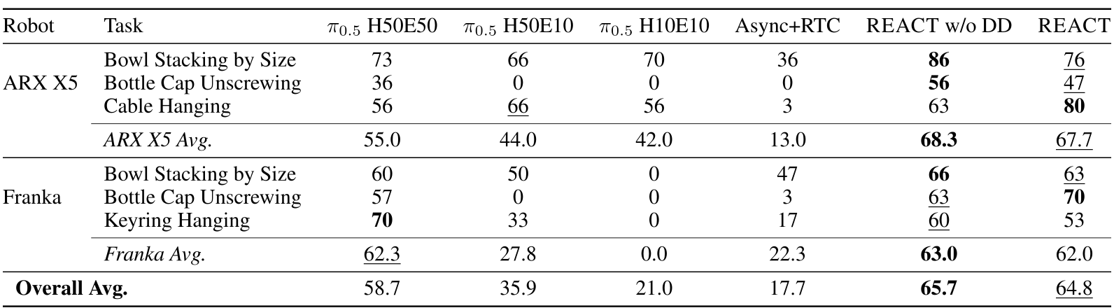
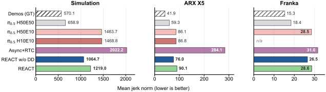
Without Dual Decoupling, REACT reaches 49.71%/20.86% clean/randomized simulation success and 65.7% real-task success, versus H50E50 at 37.43%/11.43% and 58.7%. Full REACT reaches 44.86%/19.86% and 64.8%, versus Async+RTC at 33.29%/10.57% and 17.7%. Full REACT lowers mean jerk relative to Async+RTC from 2022.2 to 1219.0 in simulation, 284.1 to 90.1 on ARX and 31.6 to 28.6 on Franka. H50E50 remains smoother overall; REACT improves the trade-off rather than every metric. H50E10 and especially H10E10 lose success despite more frequent replanning. Full REACT slightly trails its synchronous variant on these general tasks, consistent with residual cached-observation staleness. Reported two-proportion tests concern rollout sampling, not independent training seeds.

| H50E50 | H50E10 | H10E10 | Async+RTC | REACT w/o DD | REACT | |||||||
| Task | Clean | Rand | Clean | Rand | Clean | Rand | Clean | Rand | Clean | Rand | Clean | Rand |
| beat_block_hammer | 17 | 1 | 8 | 0 | 0 | 0 | 13 | 4 | 15 | 2 | 14 | 4 |
| click_bell | 61 | 6 | 71 | 18 | 35 | 0 | 64 | 8 | 89 | 32 | 61 | 22 |
| move_playingcard_away | 59 | 26 | 71 | 13 | 7 | 1 | 64 | 11 | 71 | 25 | 66 | 22 |
| pick_diverse_bottles | 20 | 3 | 9 | 0 | 0 | 1 | 10 | 6 | 27 | 9 | 33 | 6 |
| press_stapler | 58 | 23 | 22 | 3 | 9 | 4 | 37 | 13 | 67 | 42 | 63 | 39 |
| rotate_qrcode | 30 | 3 | 21 | 3 | 4 | 1 | 12 | 8 | 52 | 6 | 46 | 11 |
| turn_switch | 17 | 18 | 34 | 24 | 21 | 10 | 33 | 24 | 27 | 30 | 31 | 35 |
| Average | 37.43 | 11.43 | 33.71 | 8.71 | 10.86 | 2.43 | 33.29 | 10.57 | 49.71 | 20.86 | 44.86 | 19.86 |
4.3 Specialized Task Results
Pour Rice requires stopping a continuous pour at the target level. Full REACT succeeds in 63% of trials, versus 57% without decoupling, 3% for H50E50 and 0% for Async+RTC. Reaction Game measures stimulus-to-keypress latency: full REACT is 734±94 ms, Async+RTC 747±123 ms, the synchronous REACT variant 754±127 ms, and human teleoperation 705±73 ms. The 13 ms difference from Async+RTC is small relative to reported variability and is not shown statistically significant. Full REACT is 29 ms above the human mean under the shared apparatus; this is not a direct measurement of model computation time. Main text/caption calls the response a mouse click, whereas the detailed apparatus specifies a keyboard keypress.

4.4 Training Efficiency Analysis
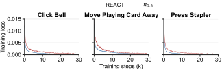
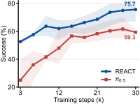
On Click Bell, Move Playing Card Away and Press Stapler, REACT reaches 52.7% average success at 3,000 updates versus 25.0% for π0.5, and matches the baseline’s 30,000-update performance after 15,000 updates. Training-loss curves and closed-loop success support efficiency measured in optimization steps. Shading denotes the range across tasks, not independent-seed uncertainty. The compared training objectives differ; lower loss and fewer steps do not establish proportional wall-clock or energy savings.
(a) Training loss over optimization steps
(b) Success vs. training steps
5 Conclusion
Persistent future actions refined across observations can preserve useful temporal context while permitting more frequent correction. The results motivate measuring observation consumption, action dispatch, task success and motion quality together, alongside raw inference latency.
6 Limitations
Validation uses only π0.5; other dual-system VLAs and video-action models remain proposed extensions. Each policy is trained for one fixed (K,S) schedule, with no evaluated zero-shot schedule switching. The authors suggest choosing S for the reaction/compute budget and a large K within the pretrained horizon, but schedule-conditioned adaptive control is future work. No independent training seeds were run. Success remains limited on randomized simulation, and asynchronous embedding age, rollout-conditioned jerk comparisons and small latency differences constrain broader claims.
Appendix A Failure Case Analysis
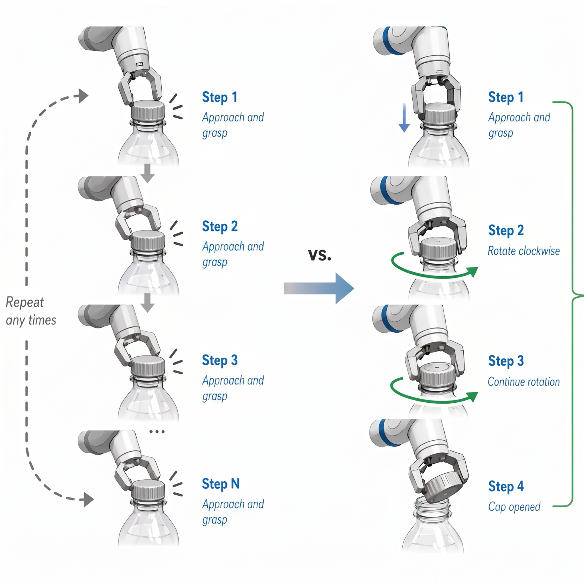
Failure examples distinguish three mechanisms. H50E50 stays smooth but can continue pouring or reaching toward an obsolete target. H50E10 may execute the approach without completing grasp–twist–release, repeatedly revisit the same contact state, or resample inconsistent intents; it has zero bottle-opening success on both robots. H10E10 additionally loses long-horizon training context and has zero success on all three Franka general tasks, so its Franka jerk is undefined. Async+RTC hides computation but still predicts from delayed state and stitches chunks; it spills rice and has high ARX jerk. Figures 6–8 retain the qualitative sequences. These examples support the authors’ interpretation, but they do not isolate action-mode switching as the sole causal explanation for every failure.

Appendix B Throughput Comparison
Throughput is counted at the policy interface: selected fresh observations consumed and executable actions dispatched. H is the prediction horizon, H_e the execution horizon, and inference cost is VLM encoding plus N action-expert steps. A high action rate can coexist with infrequent observation updates.
B.1 Qualitative Analysis
Synchronous inference adds computation time to H_e/f_control; asynchronous inference uses the larger of those times. Speeding inference helps only until execution becomes the asynchronous bottleneck. Synchronous REACT replaces N denoising steps with one per update, but still serializes VLM, DiT and S-action execution. Full REACT removes those waits through independent streams. Its rate formulas require the effective VLM pool and DiT to sustain the selected frame stream. For colocated workers, effective service rate must be measured rather than assuming worker count gives linear GPU speedup. Smaller S raises the demanded observation-processing rate.
Equations 6–15
| (6) | ||||
| (7) |
| (8) | ||||
| (9) |
| (10) | ||||
| (11) |
| (12) | ||||
| (13) |
| (14) | ||||
| (15) |
B.2 Summary of Throughput Formulas
The original formula table retains synchronous, accelerated, asynchronous and both REACT variants. Full REACT’s camera-rate output is conditional on provisioned perception and denoising throughput; input remains camera rate divided by block length.
B.3 Comparison with Typical Values
Reference measurements on a compiled RTX 4090 give VLM≈37 ms and DiT≈3 ms per step; ten-step π0.5 therefore costs about 67 ms. With H_e=50 and 30 Hz control, synchronous input is only 0.58 Hz although output is 28.8 Hz; halving inference time barely changes input to 0.59 Hz. At H_e=10, synchronous rates are 2.50/25.0 Hz and asynchronous rates 3.00/30.0 Hz. Synchronous REACT with S=10 reaches about 2.68/26.8 Hz; full REACT reaches 3/30 Hz under the stated service conditions. These schedule calculations do not measure closed-loop reaction latency or guarantee each cached embedding is current.
| Method | or | (ms) | (Hz) | (Hz) |
|---|---|---|---|---|
| Synchronous | ||||
| Synchronous | ||||
| Synchronous | ||||
| Synchronous | ||||
| Sync + Accel () | ||||
| Sync + Accel () | ||||
| Sync + Accel () | ||||
| Sync + Accel () | ||||
| Asynchronous | ||||
| Asynchronous | ||||
| Asynchronous | ||||
| Asynchronous | ||||
| REACT w/o DD () | ||||
| REACT w/o DD () | ||||
| REACT (main) | — | |||
| REACT (faster input) | — | |||
| REACT (upper bound) | — |
Throughputs are computed from unrounded cycle times; is rounded to the nearest millisecond for display. For full REACT, is not listed because the serialized inference–execution cycle is removed; after the one-time warm-up, the steady-state update period is .
Appendix C Implementation Details
Implementation details specify the robots, shared model family, training hyperparameters, initialization, scheduling assumptions and evaluation metrics.
C.1 Hardware Platforms
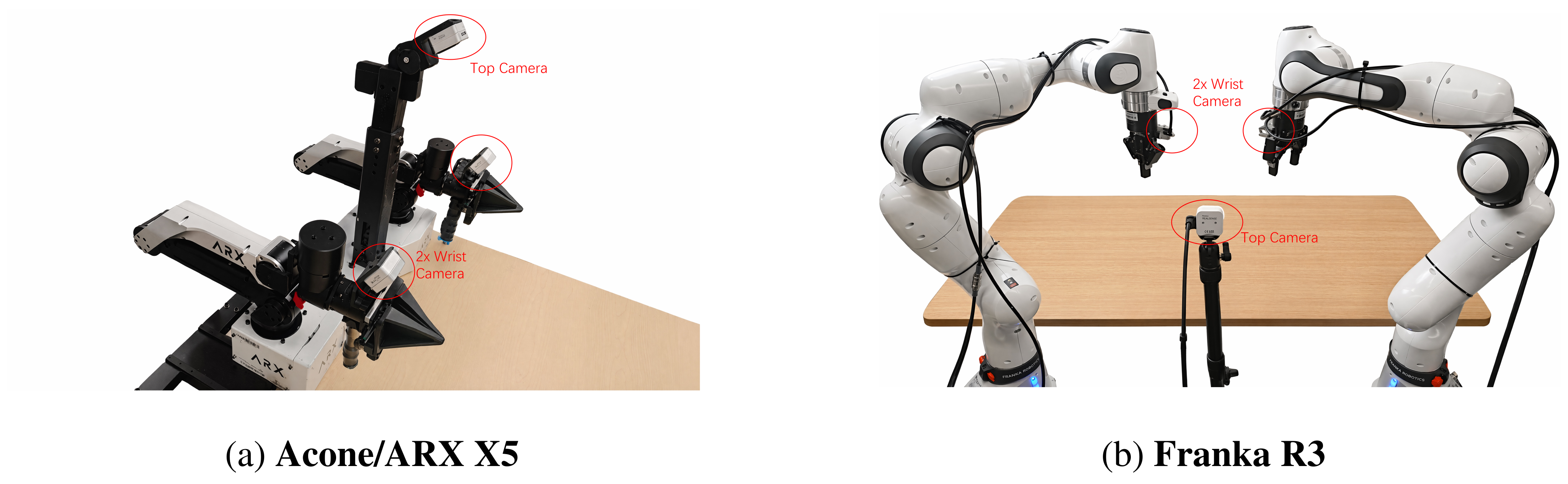
ARX X5 has two six-joint arms with parallel grippers; dual Franka Research 3 has two seven-joint arms with grippers and Cartesian impedance control. Both use front and two wrist RGB cameras and 30 Hz commands. Every evaluated deployment uses one 24 GB RTX 4090. Full REACT colocates two asynchronous VLM workers with the action expert; at the main 3 Hz selected-frame rate, the cited single-worker capacity is already sufficient. Multi-GPU deployment is supported conceptually but is not needed for the reported main configuration.
C.2 Model Architecture
π0.5 combines a PaliGemma-3B VLM/SigLIP vision encoder with a 300-million-parameter action expert. Standard baselines use ten flow steps per generated chunk; REACT uses one per rolling update and five accumulated refinements per emitted block in the main setting. ARX actions contain 12 arm-joint and two gripper coordinates; Franka actions contain two position-plus-6D-rotation poses and two gripper coordinates, totaling 20 dimensions. Main experiments use H=50; Appendix E also evaluates shorter horizons when KS<50.
C.3 Training Configuration
Training uses AdamW, peak/final learning rates 2.5×10⁻⁵/2.5×10⁻⁶, cosine decay with a 10% warm-up, weight decay 10⁻¹⁰, gradient clipping at 1 and bfloat16. Simulation uses batch size 32 for 30,000 updates; robot training uses 20 epochs, with batch 128 on ARX and 256 on Franka except 32 for Reaction Game. The complete source table retains optimizer moments and numerical settings.
| Hyperparameter | Value |
|---|---|
| Peak learning rate | |
| Final decay learning rate | |
| LR scheduler | Cosine decay with linear warmup |
| Warmup fraction | of the total training schedule |
| Optimizer | AdamW |
| AdamW | 0.9 |
| AdamW | 0.95 |
| AdamW | |
| Weight decay | |
| Simulation batch size | 32 |
| Simulation training length | 30,000 optimization steps |
| Real-robot training length | 20 epochs |
| Acone/ARX X5 batch size | 128 |
| Franka R3 batch size | 256 for all real-robot tasks except Reaction Game; 32 for Reaction Game |
| Gradient clipping | 1.0 |
| Mixed precision | bfloat16 |
C.4 Inference Configuration
Initialize each block by interpolating the reset-state action with Gaussian noise at its staircase time. Run K−1 rolling updates using the initial observation while holding the robot at its reset or safe pose; discard those front blocks. The next block has traversed all K stages, after which steady-state streaming begins. This one-time warm-up is excluded from evaluated emitted actions. Table 7 reports synchronous update latency of 66.04 ms for standard π0.5 and 39.96 ms for REACT without decoupling, a 1.65× speedup; those numbers are separate from end-to-end reaction latency.
Equation
C.5 Train-Inference Consistency
The consistency argument is a schedule invariant: advancing every block by 1/K, removing the clean front and shifting the rest returns the same staircase of time-position pairs; fresh tail noise occupies τ=1. Every query therefore uses a supervised pair. A block traverses all K stages across updates. This proves the grid alignment, not that changing observations or model-generated intermediate actions have the same distribution as corrupted demonstrations, nor a guarantee of closed-loop stability.
C.6 Benchmarks and Evaluation Protocol
The seven simulated tasks are hammering a block, clicking a bell, moving a playing card, picking diverse bottles, pressing a stapler, rotating a QR code and turning a switch. Train on demo_clean and evaluate clean plus randomized conditions, 100 rollouts each. Both real platforms perform size-ordered bowl stacking and bottle-cap unscrewing; ARX adds cable hanging and Franka keyring hanging. Each platform-task pair has 30 trials with shared randomized placements across methods. These are selected tasks rather than the full 50-task benchmark.
C.7 Evaluation Metrics
Success is completed trials divided by attempts. Smoothness is the average Euclidean norm of joint jerk, estimated by repeated central differences and averaged over successful episodes only; failed trajectories are not represented in that metric. Reaction Game uses one monotonic-clock script: record the green frame’s commitment to the display buffer, then an operating-system keyboard event when the gripper presses a designated key. The same monitor, keyboard and teleoperated robot provide the human comparison. Shared hardware controls common delays, but subtracting human mean latency does not separately identify every policy-induced delay. Pour Rice reports task success.
Appendix D Full Trajectory Smoothness Results
All per-task jerk values are retained, including undefined entries when no episode succeeds. Demonstration averages are 570.1 in simulation, 41.9 on ARX and 15.3 on Franka. Full-horizon H50E50 is closest overall, while full REACT substantially improves over Async+RTC. Because each policy contributes its own successful subset, low jerk should be interpreted jointly with success rate rather than as an unconditional motion-quality ranking.
| Setting | Task | H50E50 | H50E10 | H10E10 | Async+RTC | REACT w/o DD | REACT |
|---|---|---|---|---|---|---|---|
| Simulation | beat_block_hammer | 463.4 | 996.7 | – | 1755.0 | 664.0 | 775.9 |
| click_bell | 502.4 | 1087.2 | 1341.8 | 1946.4 | 690.8 | 712.0 | |
| move_playingcard_away | 814.3 | 2012.7 | 1784.5 | 1832.2 | 1165.8 | 1341.8 | |
| pick_diverse_bottles | 857.7 | 1391.2 | – | 1688.0 | 1253.4 | 1621.8 | |
| press_stapler | 567.9 | 1295.5 | 1425.7 | 3168.2 | 1136.4 | 1204.7 | |
| rotate_qrcode | 965.5 | 1663.9 | 1638.8 | 1944.5 | 1296.1 | 1422.3 | |
| turn_switch | 441.1 | 1798.8 | 1153.1 | 1821.2 | 1246.7 | 1454.3 | |
| Simulation Avg. | 658.9 | 1463.7 | 1468.8 | 2022.2 | 1064.7 | 1219.0 | |
| ARX X5 | Bowl Stacking by Size | 55.3 | 76.8 | 78.5 | 189.3 | 70.9 | 80.3 |
| Bottle Cap Unscrewing | 53.7 | – | – | – | 69.4 | 87.3 | |
| Cable Hanging | 68.9 | 95.4 | 95.0 | 378.8 | 87.6 | 102.7 | |
| ARX X5 Avg. | 59.3 | 86.1 | 86.8 | 284.1 | 76.0 | 90.1 | |
| Franka | Bowl Stacking by Size | 15.1 | 27.3 | – | 28.5 | 24.3 | 27.6 |
| Bottle Cap Unscrewing | 28.1 | – | – | 34.2 | 29.8 | 30.4 | |
| Keyring Hanging | 12.1 | 29.7 | – | 32.0 | 25.5 | 27.7 | |
| Franka Avg. | 18.4 | 28.5 | – | 31.6 | 26.5 | 28.6 |
Appendix E Ablation Studies
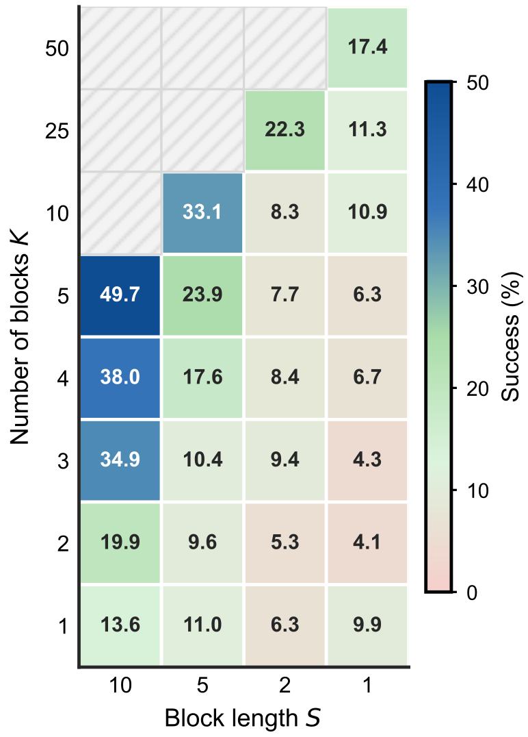
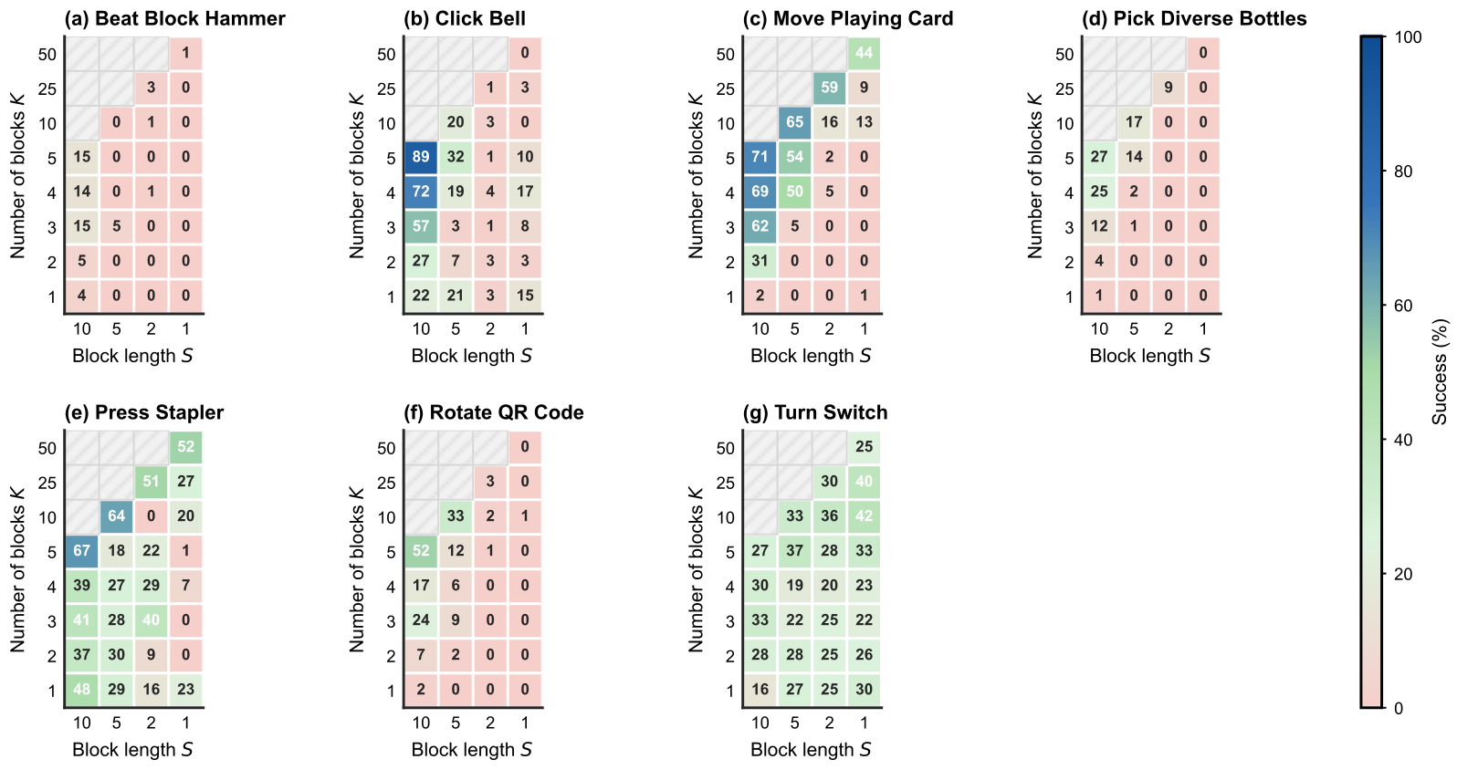
The evaluated grid restricts KS≤50 to retain the released checkpoint’s horizon; larger-horizon retraining is outside scope. The authors use S=10,K=5 throughout the main experiments, the best aggregate clean result and best or tied on six of seven tasks. At S=10, success rises from 13.6% with K=1 to 49.7% with K=5; at K=5, it rises from 6.3% with S=1 to 49.7% with S=10. Smaller blocks increase nominal observation rate but can reduce useful action context. Changing K or S also changes total horizon KS in much of this grid, so refinement count, temporal context and responsiveness are not fully isolated. K=10,S=5 provides more refinements but scores 33.1%; the recommended main configuration is empirical, not a universal optimum. The seven per-task heatmaps retain all evaluated cells, hatched exclusions and the shared color scale.
Appendix F OOD Dataset Action Prediction Open-Loop MSE
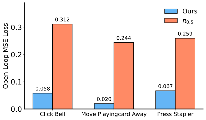
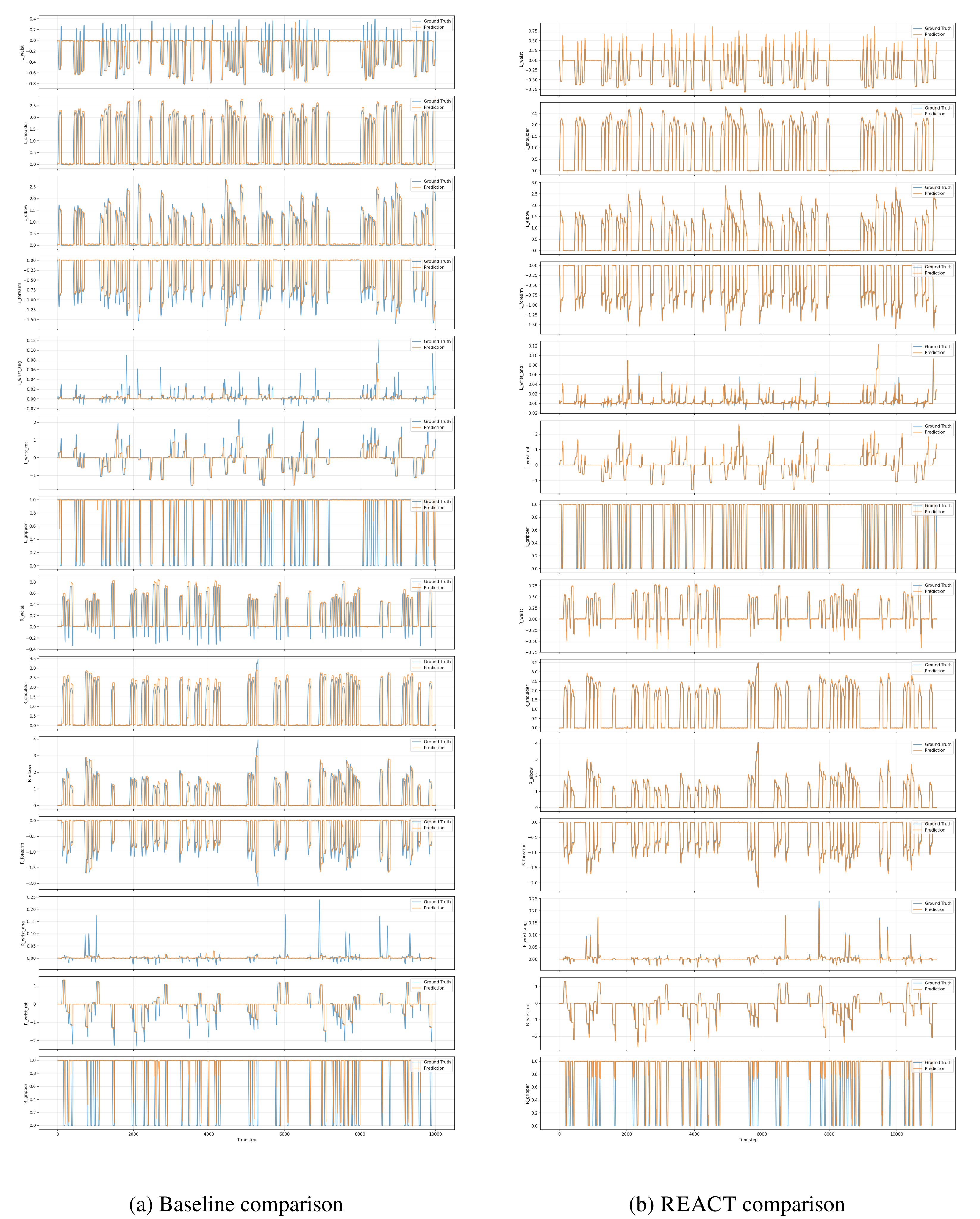
Final-checkpoint open-loop prediction on three randomized-data tasks reduces mean action MSE from 0.272 to 0.048, an 82.4% relative decrease. Task values are 0.312→0.058 for Click Bell, 0.244→0.020 for Move Playing Card Away and 0.259→0.067 for Press Stapler. The two full action-trace panels show one representative playing-card example. These are offline prediction diagnostics, distinct from closed-loop completion or training-seed robustness.