The official project and code accompany the paper. The reading separates its exact linear-system conditions from empirical nonlinear control results.
At a glance
Intuition. A model can predict the background perfectly yet fail to notice a pole beginning to fall. Avoiding a constant embedding does not guarantee that the representation preserves the unstable directions a controller must observe. This paper constructs linear examples where next-state prediction and Gaussian anti-collapse are both optimized while those directions disappear. Its remedy is endpoint inverse dynamics: recover the applied action sequence from initial and final latents, encouraging action-reachable information to survive. Exact recovery implies a strong preservation result under linearity, rich action excitation and dimension/rank conditions. In visual CartPole and Walker2D experiments, the extra loss improves feedback-relevant dynamics. The nonlinear results are empirical, use the specified observations including proprioception, and do not extend the exact linear theorem into a blanket stabilization guarantee.
1 Introduction
Feedback control needs information about directions that grow without correction. A representation may remain globally varied and predictably evolve while hiding precisely those directions. The paper therefore evaluates control-aware preservation separately from anti-collapse and prediction quality, using both linear analysis and nonlinear visual tasks.
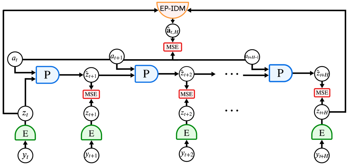
Figure 1: Architecture of our proposed world model. At each step, an encoder ()
maps observation to a latent state , and a predictor ()
rolls out latent predictions
conditioned on actions. Training losses are applied at each predicted latent: 1SP/MSP
(single- or multi-step prediction) aligns with the
encoded ground-truth . The EP-IDM estimates the intermediate actions
from and .
2 Related Work
The work connects latent JEPA prediction with detectability and stabilization. Prior inverse-dynamics objectives already used action information; this endpoint version reconstructs an entire action block and analyzes which reachable state directions that requirement preserves.
3 Setup
The physical system, observation encoder and latent predictor are separate objects. Observations can contain images and proprioception; experiments use motion information from consecutive frames plus the stated state measurements. Standard prediction and marginal anti-collapse do not specify which physical variables must be recoverable.
Equations 1–7
(1)
(2)
(3)
(4)
(5)
(6)
(7)
4 Prediction Does Not Guarantee Stabilization
A latent controller may stabilize its own predicted state while the true physical state diverges in an omitted unstable direction. The linear setup makes this failure precise under stabilizable physical dynamics and observable raw measurements, separating insufficient learned representation from an inherently uncontrollable system.
Equations 8–10
(8)
(9)
(10)
4.1 Necessary and Sufficient Conditions for Stabilization of LDS
A controller using the encoded history can stabilize the analyzed linear system exactly when the encoded observation is detectable: every invisible mode must already decay without feedback. The criterion includes marginally stable as well as unstable modes. It concerns available information, not the performance of an arbitrary learned controller.
Equation 11
(11)
4.2 The Collapse of Unstable Modes
The counterexample discards unstable coordinates and whitens a predictable stable component. It can achieve zero one-step error and the desired Gaussian latent law while losing the information required for stabilization. Thus neither a rich marginal distribution nor perfect latent prediction alone certifies control relevance.
Equations 12–13
(12)
(13)
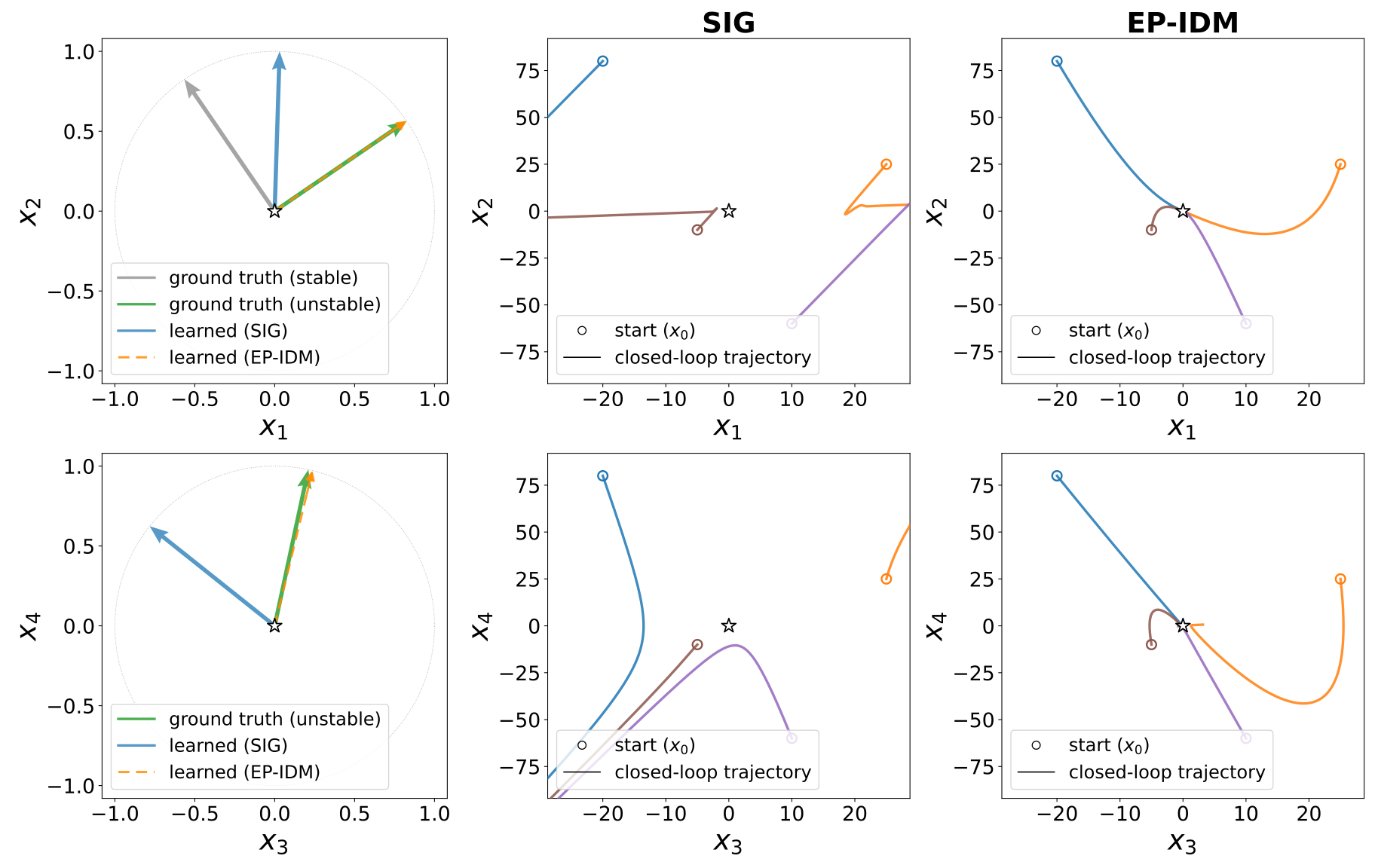
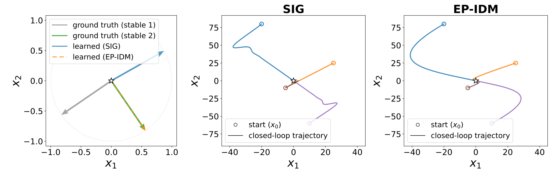
Figure 2: SIG vs. EP-IDM across two examples. Each row compares a
representation trained with SIGReg (SIG) against one trained with the
endpoint inverse-dynamics (action-reconstruction) loss (EP-IDM).
Top row: synthetic open-loop unstable LDS.Bottom row: linearized CartPole.Left: true unstable (, green) and stable (, grey)
eigenvectors versus the learned predictor’s dominant eigenvector, for SIG
(blue) and EP-IDM (dashed orange). Center: closed-loop trajectories
under the latent LQR controller from four initial states (circles) for the
model trained with SIGReg. Right: closed-loop trajectories under
the latent LQR controller for the model trained with the inverse dynamics
loss (EP-IDM). For the bottom row , and corresponds to the pole angle and angular velocity, respectively. The latent dimension is one for the example in the top row and three for the example in the bottom row.
.
5 Preserving Unstable Directions Through Inverse Dynamics
The added endpoint objective asks the initial and final latent pair to explain which action sequence produced the transition. This encourages the encoder to retain action-induced changes rather than merely predictable passive variation.
5.1 Endpoint Inverse Dynamics
An inverse model reconstructs the stacked action block from endpoint latents. It is trained jointly with the encoder and predictor. In practice this is a soft objective; zero reconstruction loss is not assumed to be attainable for long arbitrary action sequences.
Equation 14
(14)
5.2 Preservation of Reachable Directions
For affine encoding and inverse dynamics, exact endpoint action recovery under rich conditional action excitation forces preservation of the finite-horizon reachable subspace. The condition requires enough endpoint information and rank: arbitrary action blocks cannot be recovered when their dimension exceeds the state or latent capacity. The empirical loss remains useful as a bias even outside this ideal regime.
Equations 15–16
(15)
(16)
5.3 Reachability and Unstable Dynamics
Longer-horizon controllability Gramians increasingly weight controllable unstable directions under the paper’s strengthened growth and non-cancellation assumptions. Their dominant subspaces then approach the unstable subspace. Mere reachability without those conditions is not the full theorem, and extending the horizon does not override the endpoint reconstruction rank constraint.
Equations 17–19
(17)
(18)
(19)
6 Experiments
Experiments compare one- and multi-step prediction, Gaussian regularization and several action-reconstruction variants. Local linear feedback, gradient planning and sampling-based planning test different uses of the same model.
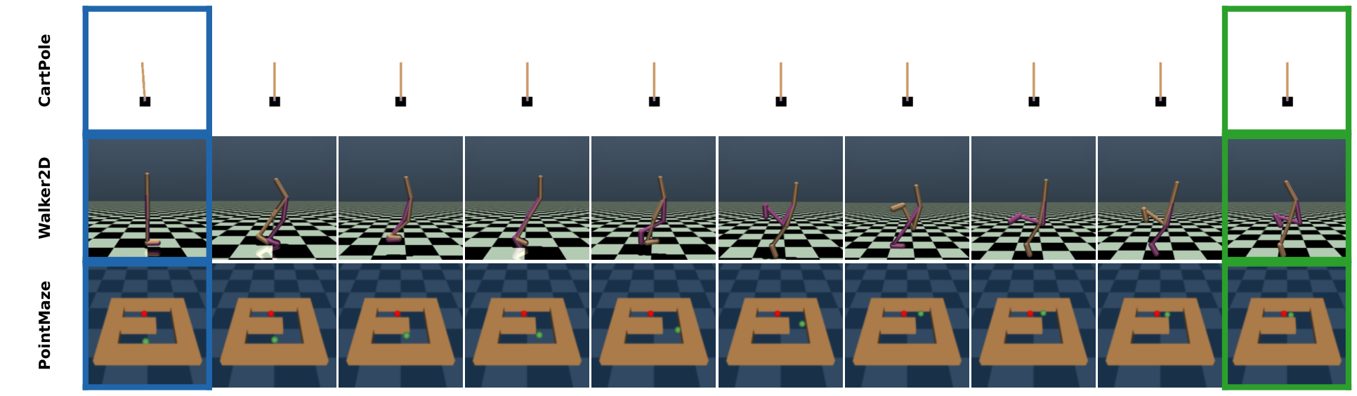
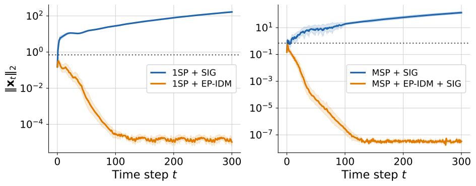
Figure 3: CartPole, Walker2D, and PointMaze visual-control tasks used in our evaluation. Each row depicts ten frames from a successful trial (initial state: blue border, final state: green border). CartPole: a continuous-action inverted-pendulum balancing task controlled via LQR. Walker2D: a bipedal robot locomotion task controlled via iCEM (Pinneri et al., 2021). PointMaze: a 2-D point-mass robot navigation task planned via CEM.Figure 4: CartPole state norm under the designed latent LQR controller over steps.
6.1 Setup
CartPole tests an unstable equilibrium, Walker2D a feedback-maintained walking cycle, and PointMaze a stable goal-reaching system. Controllers include latent LQR and nonlinear planning. Data, proprioception and action contexts are specified because they materially affect which control information is available.
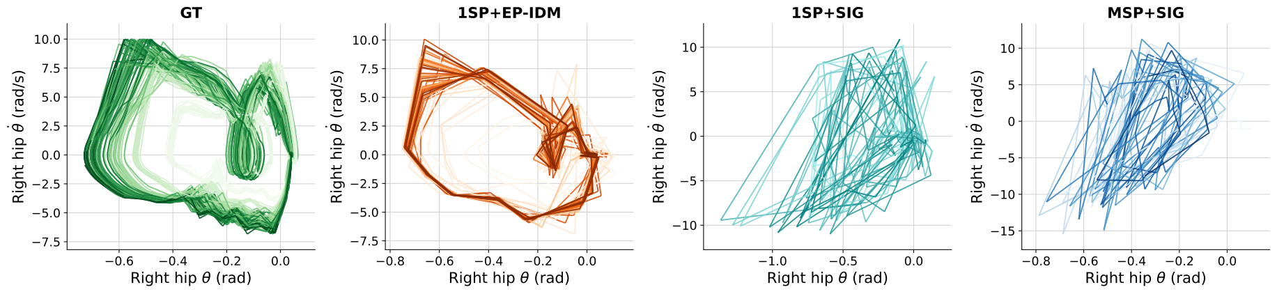
Figure 5: Walker2D. Phase portraits of right-hip angle vs. angular velocity for GT dynamics, 1SP+EP-IDM, 1SP+SIG, and MSP+SIG. Each trajectory is a -step closed-loop rollout: GT uses real MuJoCo physics, model panels roll out in latent space under an MLP-decoded state, with a SAC (Huang et al., 2022; Haarnoja et al., 2018) policy acting on the decoded observation.
6.2 CartPole: Stabilization Around an Unstable Equilibrium
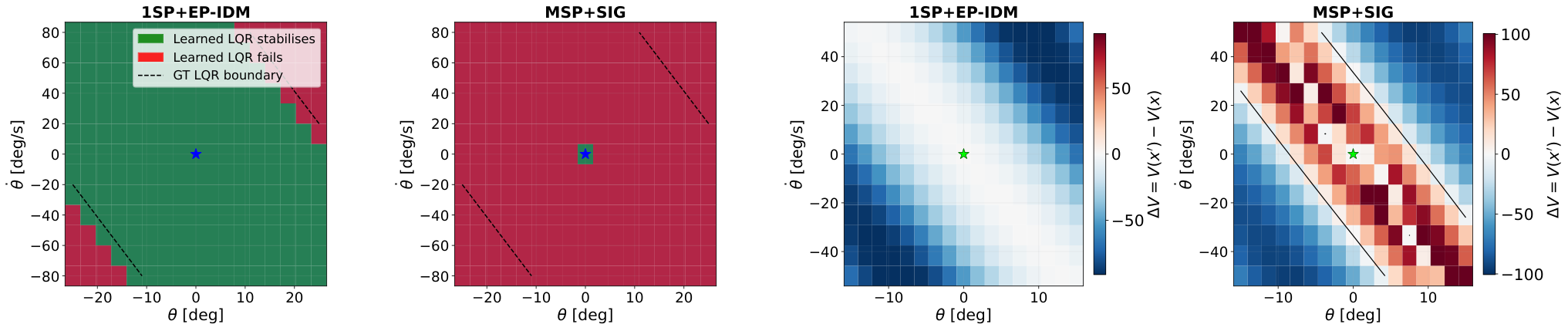
Endpoint action reconstruction changes reported latent-LQR CartPole success from zero to 100% in the small evaluated setting. Some SIGReg models still succeed with nonlinear replanning, so failure of a local linear controller should not be misreported as failure of every possible planner.
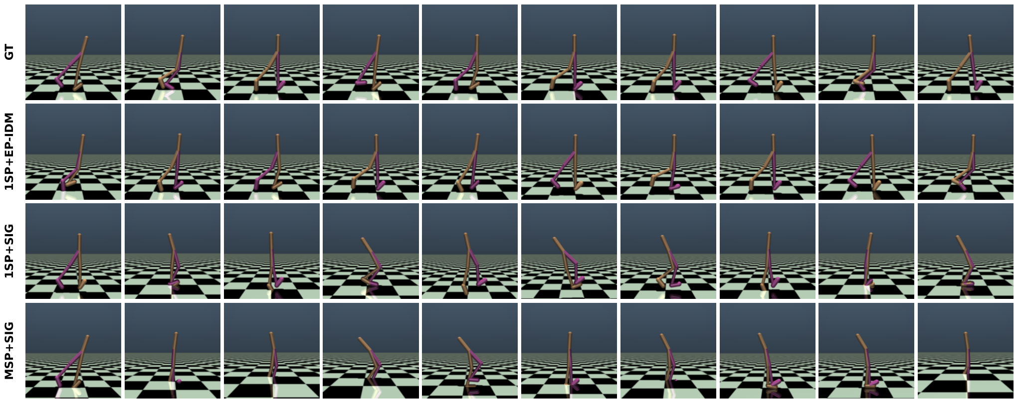
Endpoint-reconstruction models better preserve the studied gait’s cyclic structure and support stronger forward locomotion than the compared prediction-only variants. Phase portraits, decoded rollouts and control metrics test complementary aspects of the learned dynamics; the linear equilibrium theorem does not prove this nonlinear orbit result.
Figure 6: Trajectory frames for Walker2D. Each row shows ten frames uniformly sampled from a -step closed-loop rollout under the SAC policy (Haarnoja et al., 2018), decoded from the trained model’s latent state via an MLP decoder.
Table 2: Walker2D locomotion under latent iCEM (Pinneri et al., 2021).
All metrics are averaged over ten trials. Final height is the torso height (m) at the end of the episode.
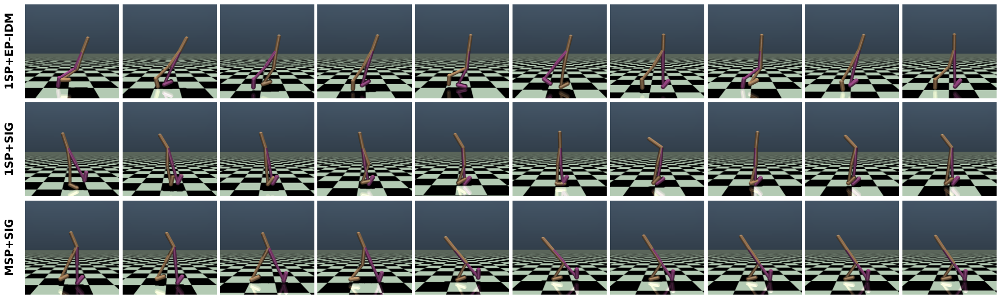
Figure 7: Planning trajectory frames for Walker2D. Each row shows ten frames uniformly sampled from a -step closed-loop rollout under latent iCEM planning for the trained models. We select the best trial, with respect to the forward displacement, across the ten trials for the trained models.
6.4 Diagnostics
Vector fields, local rollout error, attraction regions and Lyapunov differences explain why similar-looking goal costs can support different feedback controllers. PointMaze shows that action reconstruction can also preserve useful state geometry in a system without unstable modes. Diagnostics remain empirical over sampled states.
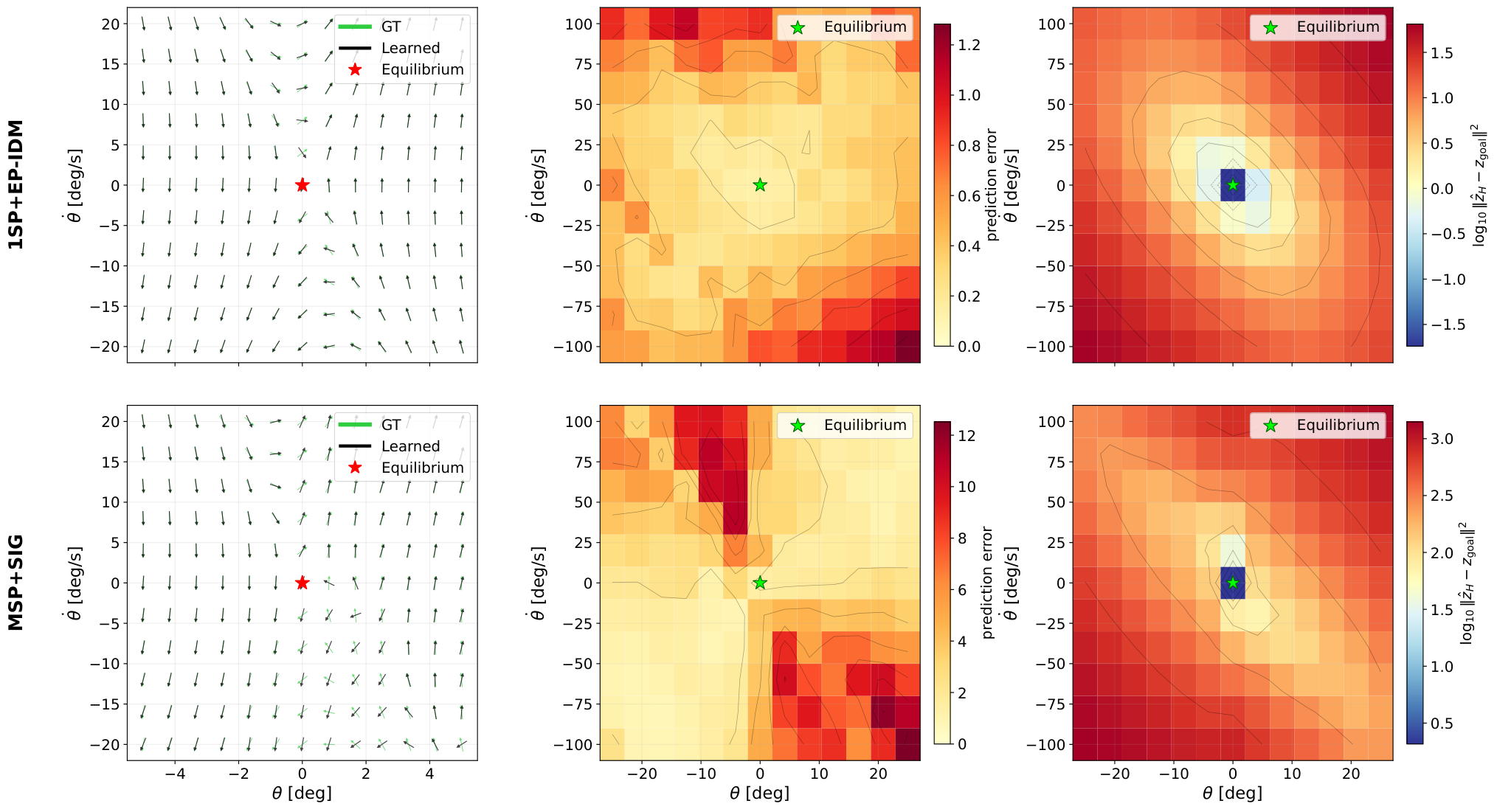
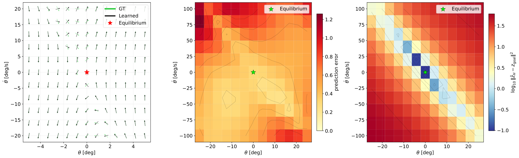
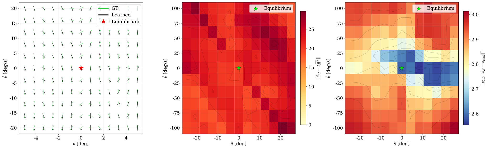
Figure 8: CartPole diagnostics.
Left: Phase portraits of ground-truth and learned vector fields.
Center: open-loop prediction error across
.
Right: Zero-action planning cost.
Because MuJoCo is non-differentiable, we estimate gradients with SPSA using two rollouts per optimization step (Spall, 1998).
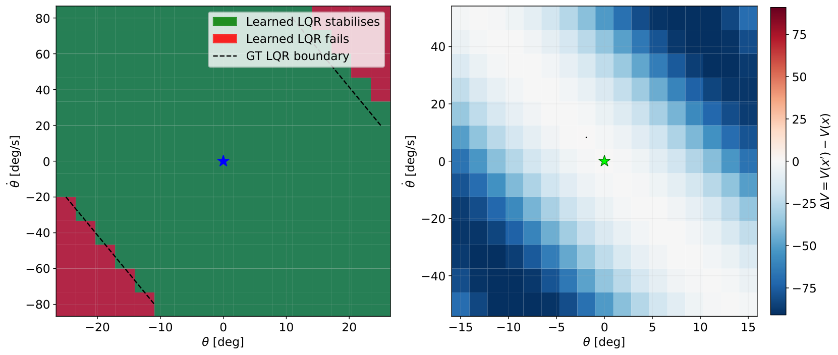
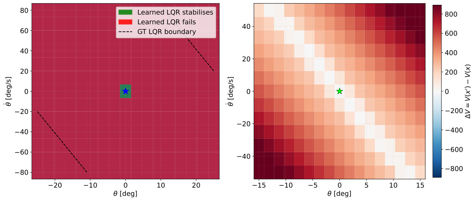
Figure 9: Local stability on CartPole.
First two panels: Empirical region of attraction of the learned LQR controller when deployed in the ground-truth system. The dashed line
indicates the ground-truth LQR boundary.
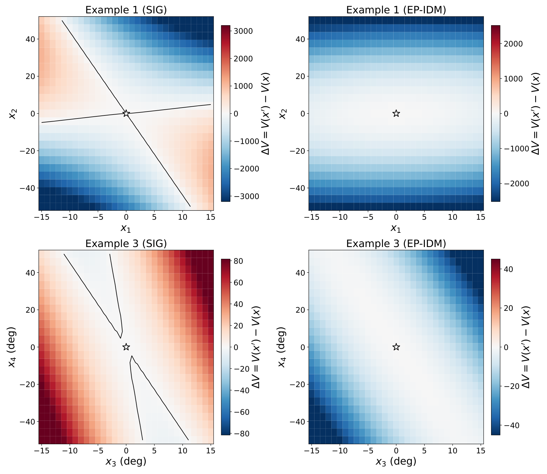
Last two panels: Lyapunov decrease under the latent LQR controller.
7 Conclusion and Future Work
The central separation is between noncollapsed predictability and information sufficient for feedback stabilization. Endpoint inverse dynamics supplies a control-aware learning signal, with an exact theorem only under restrictive linear and rank conditions. Broader nonlinear stability guarantees and combinations with planning-geometry objectives remain open.
8 Acknowledgments
Acknowledgments and funding disclosures are preserved as source context. They do not change the theorem assumptions or experimental scope.
Appendix A Appendix
The appendix retains additional rollouts, frozen-encoder tests, implementation details, ablations, linear counterexample constructions and complete proofs.
Additional diagnostics distinguish rollout fidelity, informative latent costs and stable local feedback. None is a substitute for checking the physical closed-loop trajectory.
A.1.1 CartPole
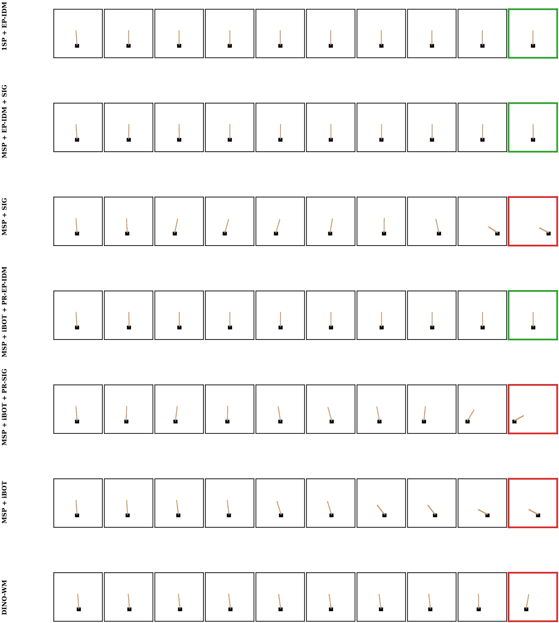
CartPole sequences and attraction-region plots compare models trained from scratch and models with frozen visual features. Endpoint reconstruction often helps, while a visually plausible goal cost alone may still yield an unstable latent-LQR controller.
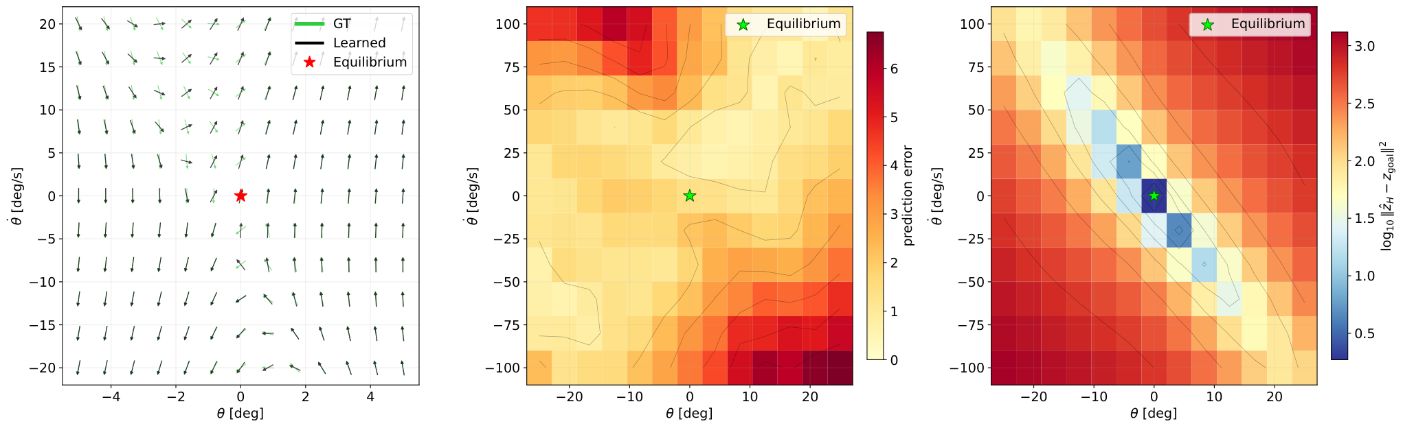
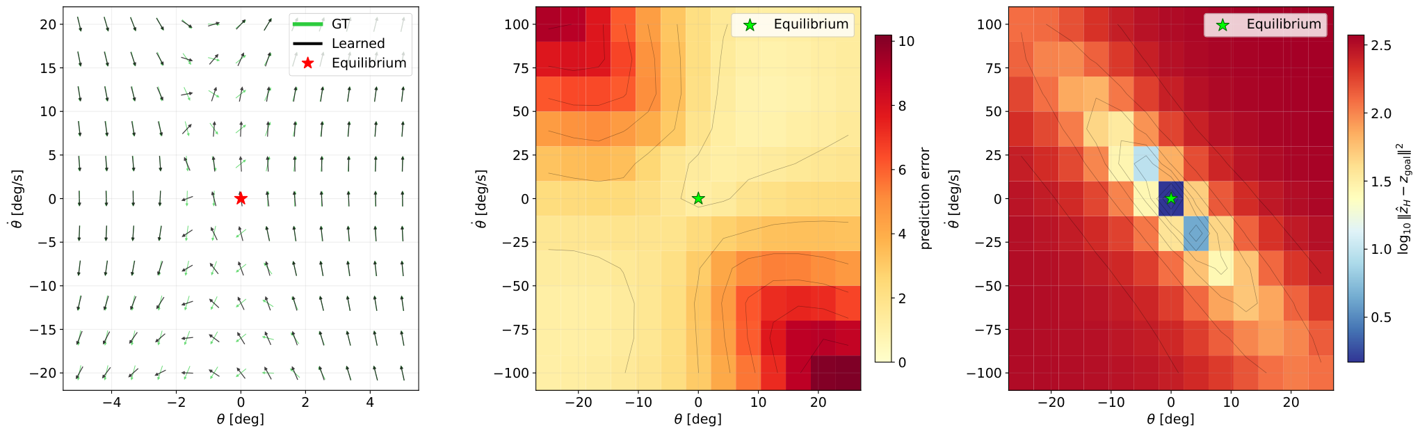
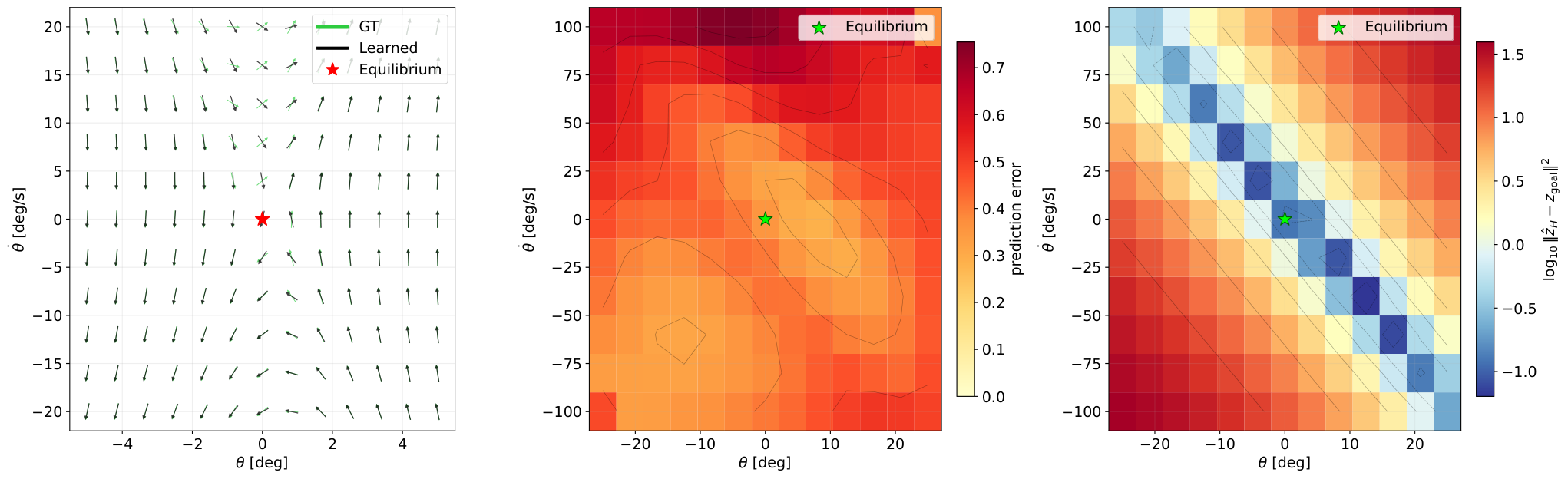
Figure 10: CartPole trajectory visualization for the trained models under the latent LQR controller.Figure 11: MSP+EP-IDM+SIG model on CartPole.
Left: Phase portrait of ground-truth vs. learned vector fields. Center: open-loop prediction error. Right: Zero-action planning cost.
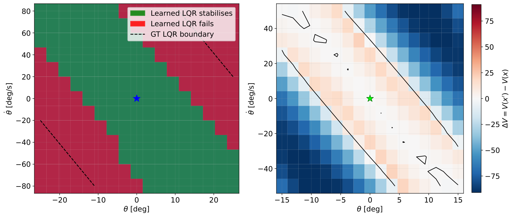
Figure 12: Local stability of MSP+EP-IDM+SIG on CartPole. Left: Empirical region of attraction (ROA) of the learned LQR policy in the GT environment. Dashed line: GTLQR boundary. Right: Lyapunov decrease under the learned policy using the GTDARE solution.Figure 13: MSP+IBOT+PR-EP-IDM model on CartPole. Panel descriptions are in Fig. 11.
Figure 14: Local stability of MSP+IBOT+PR-EP-IDM on CartPole. Panel descriptions are the same as those in Fig. 12.Figure 15: MSP+IBOT+PR-SIG model on CartPole.
Panel descriptions are the same as those in Fig. 11.
Figure 16: MSP+IBOT model on CartPole. Panel descriptions are the same as those in Fig. 11.
Figure 17: Local stability of MSP+IBOT on CartPole. Left: Empirical region of attraction (ROA) of the learned LQR policy in the GT environment. Panel descriptions are as those in Fig. 12.Figure 18: DINO-WM model on CartPole. Panel descriptions are the same as those in Fig. 11.
Table 4: CartPole CEM diagnostic metrics (action context 1).
: inverse squared mean stabilization length.
FE: final error .
PR denotes a learned projector on top of the frozen encoder.
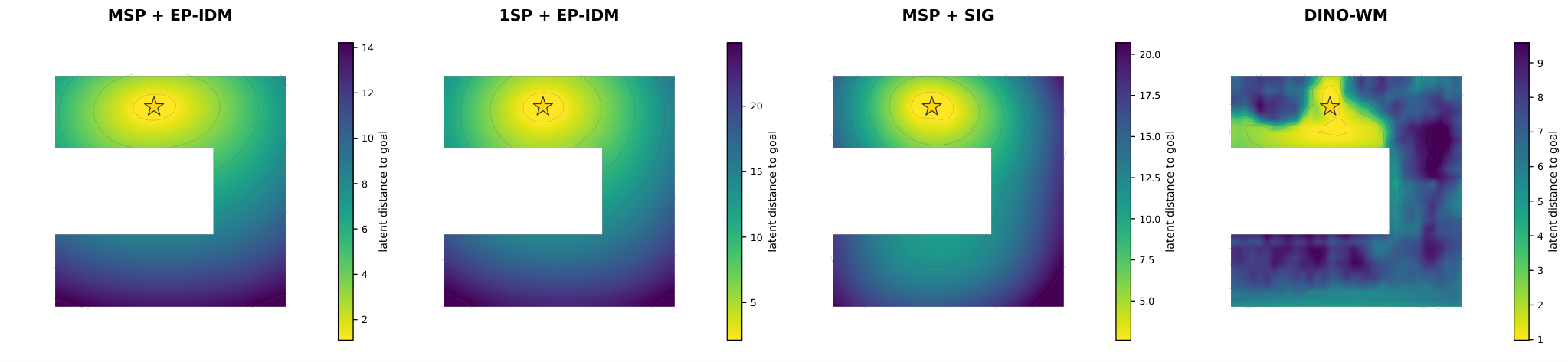
PointMaze does not require preserving an unstable subspace. Its goal-distance maps show whether the representation gives the nonlinear planner an informative route cost, providing a complementary test of action-relevant geometry.
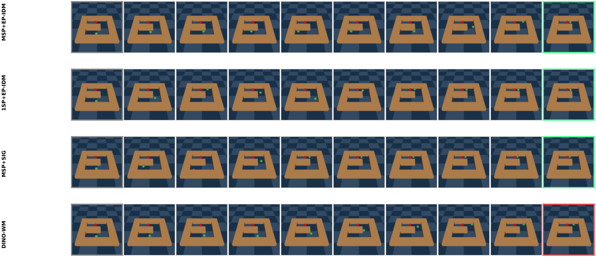
Figure 19: PointMaze visualization for our trained models under CEM planning.Figure 20: Latent goal-distance fields across the PointMaze U-maze for four trained world models.
A.1.3 Closed-Loop Prediction Error
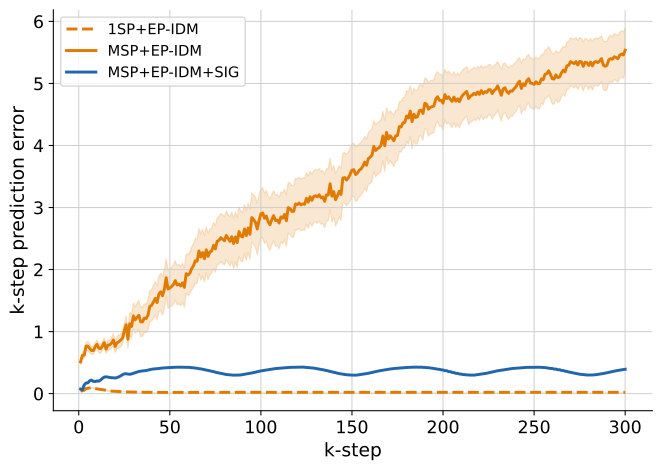
Long closed-loop prediction traces show that multi-step training alone need not prevent drift. Combining action reconstruction and marginal regularization can improve different aspects of the model; one-step error is not a complete summary of either.
Figure 21: -step closed-loop prediction error along trajectories generated by the ground-truth LQR controller. Curves show the physical-state error between the ground-truth trajectory and the trajectory decoded from each latent rollout.
A.2 Pre-trained encoders
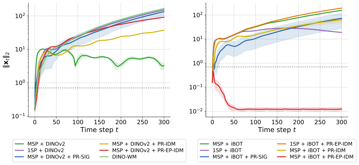
A learned projector can retain useful control information present in a frozen backbone, but cannot reconstruct information the backbone has already removed. The iBOT and DINOv2 comparisons illustrate this limitation and the distinction between LQR and nonlinear-planning success.
Table 5: CartPole control performance with frozen pretrained
encoders. SR: success rate. MFS: mean fraction of steps within the success
threshold. PR denotes a learned projector. DINO-WM (Zhou et al., 2024)
is an external baseline.
Figure 22: CartPole state norm under the learned latent LQR
controller over steps. Left: DINOv2. Right: iBOT.
A.3 Additional Details on the Implementation of our Experiments
The reproducibility section specifies perception, action decoding, datasets and controller budgets. These choices constrain the meaning of the nonlinear evidence.
A.3.1 Model Architecture
The from-scratch encoder combines frame-difference information and proprioception into a compact latent. Predictor and action-decoder architectures are retained. Calling the task visual does not mean every experiment excludes measured physical-state information.
Table 6: Task-specific observation and action dimensions. The frame skip is the number of simulator steps represented by one model transition.
Task
Image size
Proprioception
Action
Frame skip
Training trajectories
CartPole
Walker2D
PointMaze
Table 7: World-model training hyperparameters.
Hyperparameter
Value
Hyperparameter
Value
Optimizer
AdamW
Epochs
Batch size
Prediction horizon
Initial learning rate
Minimum learning rate
Weight decay
Warm-up epochs
Gradient-norm threshold
Latent dimension
Random seed
Active loss weights
A.3.2 Task and Dataset Details
Dataset mixtures include passive, random and stabilizing behavior, with separate training, validation and test trajectories. The small number of tested initial conditions limits interpreting perfect success as a broad probabilistic guarantee.
A.3.3 Planning and Control Details
LQR relies on local linearization; CEM, improved CEM and gradient planning optimize finite action sequences. The Walker2D improved-CEM setup uses the stated policy warm start, which is an important additional resource.
Table 8: CEM and improved-CEM planning hyperparameters. Here, “execute” denotes the number of actions applied before replanning.
SIGReg matches sampled scalar projections of the latent distribution to a Gaussian reference. This discourages global collapse but does not directly encode a detectability or controllability constraint.
Equations
A.3.5 Additional Action Reconstruction Losses
One-step, multi-step-trajectory and endpoint inverse dynamics expose the action decoder to different latent information. Their losses are not equivalent: an entire intermediate trajectory may reveal actions that endpoints alone cannot distinguish.
Equations 20–24
(20)
(21)
(22)
(23)
(24)
A.4 Ablations
The ablations vary inverse-dynamics formulation, action-history length, proprioceptive inputs and regularization. They qualify attributing every gain to the endpoint architecture and demonstrate interactions with available observation information.
Table 9: CartPole ablation over inverse-dynamics formulations for an encoder trained from scratch.
Table 13: CartPole ablation with a frozen iBOT encoder and action
context five, with and without proprioceptive inputs. PR denotes the learned projector. SR: success rate, held: fraction of trials in which stabilization is preserved.
Table 14: Ablation on the encoder gain as a function of initial-state perturbation magnitude . We start from a perturbed upright equilibrium, the cart pole is stepped with zero action for 60 steps. We measure the mean latent displacement divided by the mean physical-state displacement .
Encoder
iBOT
1.07
1.11
1.07
1.07
1.02
1.03
DINOv2
25.45
26.07
26.38
25.67
21.83
25.12
Table 15: Fixed-point residual of the learned predictor at the encoded
upright CartPole equilibrium under zero action. The residual measures the one-step drift from this encoded equilibrium. PR denotes a learned projector on top of the frozen encoder.
Explicit linear systems and perceptual mixing maps show how an encoder can discard unstable coordinates without failing its training objectives. A stable-system example separates control relevance from instability specifically. These are constructed counterexamples, not empirical estimates of how often collapse occurs.
Equations 25–31
(25)
(26)
(27)
(28)
(29)
(30)
(31)
Figure 23: Synthetic open-loop stable LDS. This example considers a two-dimensional open-loop stable system. Panels descriptions are the same as those in Fig. 2.Equations 32–35
(32)
(33)
(34)
(35)
Figure 24: Sign of after one closed-loop step under the learned latent LQR controller, where and is the
ground-truth Lyapunov function matrix. We also depict the contour (separatrix), i.e., the boundary separating states where the learned controller decreases (blue) from those where it does not (red).
A.6 Proofs of Our Theoretical Guarantees
The proofs retain the supporting rank, subspace and perturbation results. Their linear-algebra conditions should accompany any statement of exact preservation or convergence.
A.6.1 Supporting Lemmas
Exact affine reconstruction on an open set forces an observation map to have a left inverse on the reconstructed coordinates. Matrix perturbation results subsequently relate dominant Gramian eigenspaces to the unstable subspace.
Equations 36–37
(36)
(37)
A.6.2 Proof of Lemma 1
If an invisible unstable direction separates two states, a controller receiving identical encoded histories cannot distinguish them, while their difference grows. Detectability rules out this obstruction and supplies the converse linear feedback argument under the stated system assumptions.
Equations 38–40
(38)
(39)
(40)
A.6.3 Proof of Theorem 1
Unrolling linear dynamics expresses endpoint changes through the finite-horizon controllability matrix. Exact recovery of a richly excited action block forces its encoded image to retain rank, which prevents the encoder from annihilating reachable directions. The required rank may be impossible at large action-block dimension.
Equations 41–43
(41)
(42)
(43)
A.6.4 Proof of Theorem 2
The Gramian proof separates stable and unstable contributions and bounds their growth and coupling before applying subspace perturbation arguments. Uniform expansion, sufficient excitation and non-cancellation conditions are material assumptions; they are stronger than merely stating that an unstable mode is controllable.
Equations 44–61
(44)
(45)
(46)
(47)
(48)
(49)
(50)
(51)
(52)
(53)
(54)
(55)
(56)
(57)
(58)
(59)
(60)
(61)
41 references
Ames et al. (2014)A. D. Ames, K. Galloway, K. Sreenath, and J. W. GrizzleRapidly exponentially stabilizing control lyapunov functions and hybrid zero dynamics.
IEEE Transactions on Automatic Control59 (4), pp. 876–891.
Ames et al. (2016)A. D. Ames, X. Xu, J. W. Grizzle, and P. TabuadaControl barrier function based quadratic programs for safety critical systems.
IEEE transactions on automatic control62 (8), pp. 3861–3876.
Assran et al. (2023)M. Assran, Q. Duval, I. Misra, P. Bojanowski, P. Vincent, M. Rabbat, Y. LeCun, and N. BallasSelf-supervised learning from images with a joint-embedding predictive architecture.
In Proceedings of the IEEE/CVF Conference on Computer Vision and Pattern Recognition,
pp. 15619–15629.
Balestriero and LeCun (2025)R. Balestriero and Y. LeCunLejepa: provable and scalable self-supervised learning without the heuristics.
arXiv preprint arXiv:2511.08544.
Bardes et al. (2021)A. Bardes, J. Ponce, and Y. LeCunVicreg: variance-invariance-covariance regularization for self-supervised learning.
arXiv preprint arXiv:2105.04906.
Deng et al. (2009)J. Deng, W. Dong, R. Socher, L. Li, K. Li, and L. Fei-FeiImagenet: a large-scale hierarchical image database.
In 2009 IEEE conference on computer vision and pattern recognition,
pp. 248–255.
Haarnoja et al. (2018)T. Haarnoja, A. Zhou, P. Abbeel, and S. LevineSoft actor-critic: off-policy maximum entropy deep reinforcement learning with a stochastic actor.
In International conference on machine learning,
pp. 1861–1870.
Hafner et al. (2020)D. Hafner, T. Lillicrap, J. Ba, and M. NorouziDream to control: learning behaviors by latent imagination.
In International Conference on Learning Representations,
Hafner et al. (2019)D. Hafner, T. Lillicrap, I. Fischer, R. Villegas, D. Ha, H. Lee, and J. DavidsonLearning latent dynamics for planning from pixels.
In International conference on machine learning,
pp. 2555–2565.
Hafner et al. (2021)D. Hafner, T. P. Lillicrap, M. Norouzi, and J. BaMastering atari with discrete world models.
In International Conference on Learning Representations,
Hu et al. (2022)Y. Hu, A. Wierman, and G. QuOn the sample complexity of stabilizing lti systems on a single trajectory.
Advances in Neural Information Processing Systems35, pp. 16989–17002.
Huang et al. (2026)H. Huang, Y. LeCun, and R. BalestrieroLlm-jepa: large language models meet joint embedding predictive architectures.
In International Conference on Learning Representations,
Vol. 2026, pp. 105717–105737.
Huang et al. (2022)S. Huang, R. F. J. Dossa, C. Ye, J. Braga, D. Chakraborty, K. Mehta, and J. G. AraújoCleanrl: high-quality single-file implementations of deep reinforcement learning algorithms.
Journal of Machine Learning Research23 (274), pp. 1–18.
Ivashkov et al. (2026)P. Ivashkov, R. Balestriero, and B. SchölkopfSensorimotor world models: perception for action via inverse dynamics.
arXiv preprint arXiv:2606.20104.
Kuang et al. (2026)Y. Kuang, Y. Dagade, Q. L. Lidec, L. Maes, R. Balestriero, and Y. LeCunLpWM: a case for sparse representations in world models.
arXiv preprint arXiv:2608.22764.
Levine et al. (2020)S. Levine, A. Kumar, G. Tucker, and J. FuOffline reinforcement learning: tutorial, review, and perspectives on open problems.
arXiv preprint arXiv:2005.01643.
Lutkus et al. (2025)P. Lutkus, K. Wang, L. Lindemann, and S. TuLatent representations for control design with provable stability and safety guarantees.
In 2025 IEEE 64th Conference on Decision and Control (CDC),
pp. 2937–2944.
Maes et al. (2026)L. Maes, Q. L. Lidec, D. Scieur, Y. LeCun, and R. BalestrieroLeworldmodel: stable end-to-end joint-embedding predictive architecture from pixels.
arXiv preprint arXiv:2603.19312.
Marco et al. (2021)A. Marco, D. Baumann, M. Khadiv, P. Hennig, L. Righetti, and S. TrimpeRobot learning with crash constraints.
IEEE Robotics and Automation Letters6 (2), pp. 1439–1446.
Mellinger and Kumar (2011)D. Mellinger and V. KumarMinimum snap trajectory generation and control for quadrotors.
In 2011 IEEE international conference on robotics and automation,
pp. 2520–2525.
Mhammedi et al. (2020)Z. Mhammedi, D. J. Foster, M. Simchowitz, D. Misra, W. Sun, A. Krishnamurthy, A. Rakhlin, and J. LangfordLearning the linear quadratic regulator from nonlinear observations.
Advances in Neural Information Processing Systems33, pp. 14532–14543.
Nath et al. (2026)D. Nath, A. Srinivasan, H. Yin, R. Jiang, J. Fang, and G. ChouPixels to proofs: probabilistically-safe latent world model control via parallel conformal robust mpc.
arXiv preprint arXiv:2606.15594.
Oquab et al. (2023)M. Oquab, T. Darcet, T. Moutakanni, H. Vo, M. Szafraniec, V. Khalidov, P. Fernandez, D. Haziza, F. Massa, A. El-Nouby, et al.Dinov2: learning robust visual features without supervision.
arXiv preprint arXiv:2304.07193.
Parthasarathy et al. (2025)A. Parthasarathy, N. Kalra, R. Agrawal, Y. LeCun, O. Bounou, P. Izmailov, and M. GoldblumClosing the train-test gap in world models for gradient-based planning.
arXiv preprint arXiv:2512.09929.
Pinneri et al. (2021)C. Pinneri, S. Sawant, S. Blaes, J. Achterhold, J. Stueckler, M. Rolinek, and G. MartiusSample-efficient cross-entropy method for real-time planning.
In Conference on Robot Learning,
pp. 1049–1065.
Sobal et al. (2025)V. Sobal, W. Zhang, K. Cho, R. Balestriero, T. G. Rudner, and Y. LeCunLearning from reward-free offline data: a case for planning with latent dynamics models.
arXiv preprint arXiv:2502.14819.
Spall (1998)J. C. SpallAn overview of the simultaneous perturbation method for efficient optimization.
Johns Hopkins apl technical digest19 (4), pp. 482–492.
Todorov et al. (2012)E. Todorov, T. Erez, and Y. TassaMujoco: a physics engine for model-based control.
In 2012 IEEE/RSJ international conference on intelligent robots and systems,
pp. 5026–5033.
Toso et al. (2026)L. F. Toso, D. Shadunts, Y. Lu, N. Sharma, D. Zhan, N. H. Nguyen, and J. AndersonLearning invariant visual representations for planning with joint-embedding predictive world models.
arXiv preprint arXiv:2602.18639.
Toso et al. (2025)L. F. Toso, L. Ye, and J. AndersonLearning stabilizing policies via an unstable subspace representation.
In 2025 IEEE 64th Conference on Decision and Control (CDC),
pp. 7543–7550.
Wang et al. (2026a)Y. Wang, O. Bounou, G. Zhou, R. Balestriero, T. G. Rudner, Y. LeCun, and M. RenTemporal straightening for latent planning.
arXiv preprint arXiv:2603.12231.
Werner and Peherstorfer (2024)S. W. Werner and B. PeherstorferOn the sample complexity of stabilizing linear dynamical systems from data.
Foundations of Computational Mathematics24 (3), pp. 955–987.
Zhang et al. (2026)W. Zhang, B. Terver, A. Zholus, S. Chitnis, H. Sutaria, M. Assran, R. Balestriero, A. Bar, A. Bardes, Y. LeCun, et al.Hierarchical planning with latent world models.
arXiv preprint arXiv:2604.03208.
Zhou et al. (2024)G. Zhou, H. Pan, Y. LeCun, and L. PintoDino-wm: world models on pre-trained visual features enable zero-shot planning.
arXiv preprint arXiv:2411.04983.
Zhou et al. (2021)J. Zhou, C. Wei, H. Wang, W. Shen, C. Xie, A. Yuille, and T. KongIbot: image bert pre-training with online tokenizer.
arXiv preprint arXiv:2111.07832.