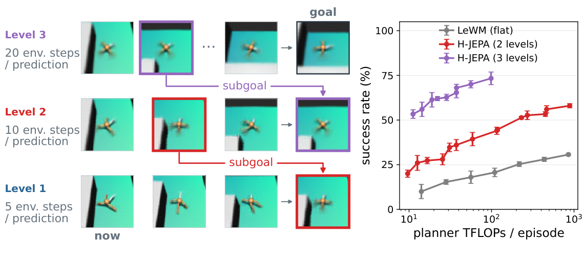
The teaser shows top-down planning across learned representation levels. Higher-level subgoals guide lower-level search instead of specifying primitive actions directly.
Figure 1: Hierarchical abstractions support planning at multiple timescales.Left: visualization of hierarchical planning in Visual AntMaze. Level 3 plans toward
the final goal in the most abstract latent space. Its first predicted state becomes
a subgoal for the level-2 planner; this decomposition recurses to the level-1 planner, which
outputs raw actions.
The first and last columns decode each level’s start and goal latents, respectively;
the middle columns decode its planned predictions. Higher-level latents retain
the ant’s position and maze layout while losing leg-pose detail. See §2.2 for the
formal planning procedure.
Right: planning success versus planner compute on AntMaze. Curves show
Pareto fronts for flat LeWM [53] and two-/three-level H-JEPA; error bars are standard error (SE) over three paired
model and planner seeds (§4.1).
At a glance
Intuition. A navigator may need to remember which corridor it is in while ignoring the exact phase of its legs. H-JEPA learns several predictive representations: higher levels look farther ahead and can discard fast detail that becomes hard to predict at that scale. A high-level plan proposes latent subgoals, and lower levels refine them into primitive actions. Unlike April’s HWM, the levels have distinct learned state spaces, not just different clocks in a shared space. Simulated planning and representation probes support this separation of temporal search and goal geometry. Diverse DROID scenes expose a further failure: a model can encode stable background identity instead of the moving robot. Inverse-dynamics supervision helps there, but the DROID results are offline plan-fidelity measurements, not closed-loop deployment on a physical robot.
1 Introduction
A shared fine-grained representation may predict local dynamics well while supplying a poor distant-goal cost. H-JEPA changes both the prediction horizon and the representation at each level. The proposed benefit therefore has two mechanisms: shorter subproblems in time and a higher-level cost that ignores some irrelevant fast detail.
2 Method
2.1 Hierarchical predictive learning
The first level encodes observations and actions. Each higher level encodes lower-level latent windows and pooled action blocks, with a stride controlling how far it advances and a window controlling what it summarizes. Each level has its own predictor and anti-collapse objective. End-to-end training allows upper-level objectives to reshape encoders below them.
Figure 2: H-JEPA training across temporal scales.
(a) With and , level 2 encodes every other level-1 state
pointwise and aggregates the intervening action embeddings.
Faded columns are retained at level 1 but skipped at level 2.
(b) Each level predicts the next latent state conditioned on preceding latent
states and actions,
with SIGReg regularizing the states against collapse.
All levels are trained end-to-end,
with gradients from upper-level objectives propagating through lower-level encoders.Equations 1–3
(1)
(2)
(3)
2.2 Hierarchical planning over learned abstractions
Planning begins at the top with a final-goal cost. Lower-level predicted states are passed through the next encoder before matching the upper level’s subgoals, so states in different latent spaces are compared through the learned hierarchy. The process reaches primitive actions at level one and repeats with new observations during receding-horizon execution.
Figure 3: Planning runs top-down through the hierarchy, and the lower level
is steered by subgoals the upper level predicted. Two-level instance () of
§2.2. Current and goal observations and
are encoded bottom-up into initial states and goal states
. Level 2 optimizes macro-actions by unrolling and matching
its final prediction to . Its predicted states become subgoals
for level 1, which optimizes primitive actions and lifts its predictions
through for comparison in level-2 latent space
(Eq. (6)).Equations 4–6
(4)
(5)
(6)
3 Learning Hierarchical Abstractions
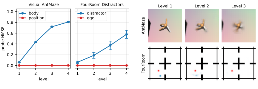
Probes compare what each frozen level retains about navigation and manipulation entities. Higher levels selectively lose fast body or distractor information when data separates those dynamics from slower task-relevant motion. That pattern is weaker when all entities evolve on similar timescales. Selective abstraction is therefore a property of the learned objective and training data, not an automatic consequence of adding layers.
Figure 4: Selective abstraction across hierarchy levels.Left: MLP-probe NMSE (mean SE over three training seeds) at
successive levels of four-level H-JEPAs on Visual AntMaze and
FourRoomDistractors. Body state or distractor position becomes less
recoverable at higher levels while agent position remains recoverable.
Right: one observation decoded from
levels –; decoders serve only for visualization.
AntMaze’s leg pose becomes less distinct; FourRoom’s blue distractor fades
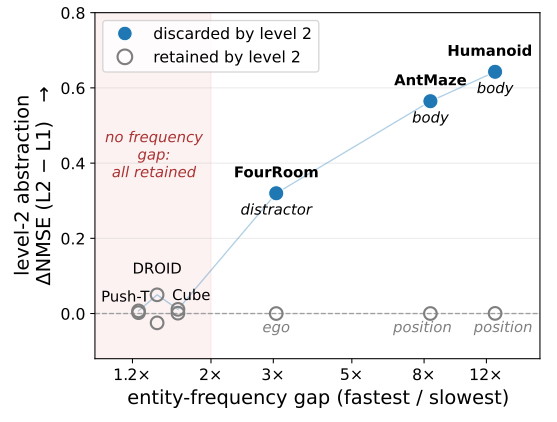
while the red agent remains visible.Figure 5: Larger temporal-frequency gaps correlate with stronger selective abstraction.
The x-axis measures temporal separation in each training dataset:
the ratio of the characteristic frequencies (spectral centroids) of the fastest-
and slowest-varying state components, shown on a log scale.
The y-axis shows the change in per-entity
probing NMSE from level 1 to level 2;
positive values indicate poorer recoverability at level 2.
Across environments, larger frequency gaps coincide with greater increases
in fast-entity probing error (filled markers), while slow-entity error remains
near its level-1 value (open markers).
Environments with gaps below (shaded region) show little selective abstraction.
4 Planning with Hierarchical Abstractions
The evaluation compares hierarchy depth and compute, isolates goal-cost geometry, and then tests diverse real-video scenes. These stages distinguish simulation success from offline imitation-of-expert-path fidelity.
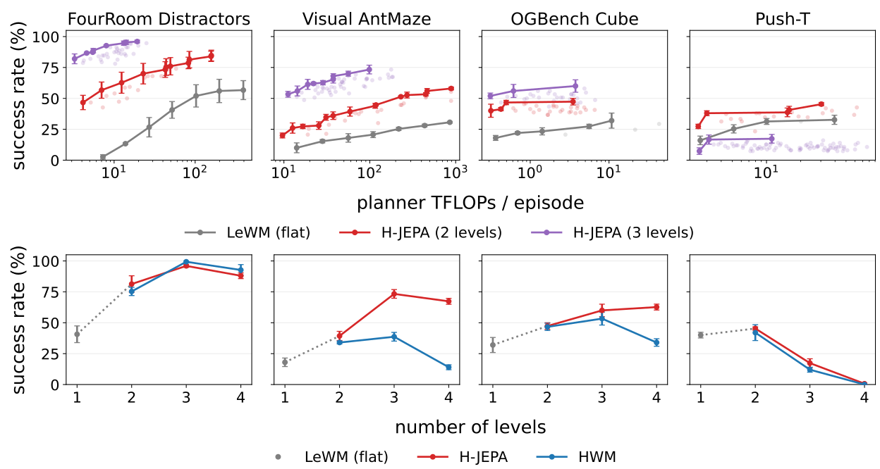
Figure 6: Gradient-based planning across compute budgets and hierarchy depths,
comparing LeWM [53], H-JEPA, and the hierarchical world model baseline
HWM [92].
Error bars in both panels show one SE over three seeds.
Top: success versus planner FLOPs per episode, sweeping action-sample counts
with other planner settings fixed. FLOPs include forward and backward passes. Bold curves are Pareto fronts.
Bottom: success versus hierarchy depth on a separate set of tasks per
environment. Planner settings are selected under a -TFLOP planning budget.
See §E for protocols and
Fig. 9 for the DROID results.
4.1 Planning performance across compute budgets and depths
Additional levels improve the compute–success frontier on several tasks, but depth is not monotonically helpful. Three-level Push-T performs poorly, plausibly because short episodes leave fewer usable training clips for the larger temporal window. Comparisons with HWM test whether distinct state representations help beyond temporal decomposition alone.
4.2 How hierarchy improves planning
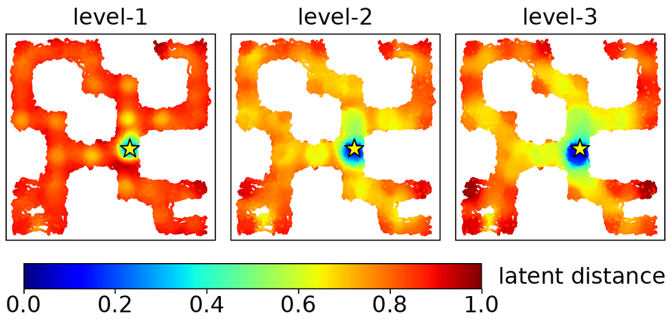
With rollout dynamics fixed, scoring plans in a higher latent space can improve AntMaze navigation, where low-level distances are nearly flat away from the goal. Hierarchical planning also divides a long route into easier subproblems. Cost-only controls show that representation geometry and temporal decomposition contribute separately, with environment-dependent benefits.
Model depth
Cost / planner
2 levels
3 levels
4 levels
Native L1
L2 projection
L3 projection
–
L4 projection
–
–
Hierarchical
Table 1: Changing only the cost on AntMaze.
Success (%, mean SE, three seeds).
Within each column, the first four rows share level-1 dynamics and planner
settings; only the cost space changes. Hierarchical planning is a separate reference.
Figure 7: Planning cost geometry on AntMaze.
Distance to anchor in each latent space of a three-level H-JEPA
(blue near, red far; one training seed).
Higher levels show more graded costs along corridors and a broader low-cost
region around the anchor.
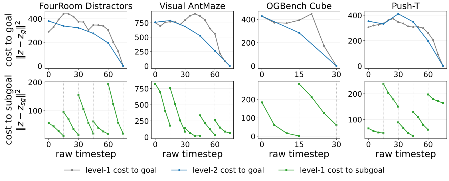
Figure 8: Temporal decomposition of planning costs. We analyze a two-level H-JEPA with . Top:Goal cost in level-1 and level-2 space. For a held-out expert trajectory we encode each frame at both levels,
and compute the distance between each timestep’s latent and the
goal (final-timestep) latent, . At level 2 we subsample
at the training stride. Bottom:Subgoal
tracking cost. The level-2 subgoals are the level-2 latents at the subsampled
timesteps. Within each subgoal segment we re-anchor the level-1 rollout from the encoded latent at the segment start, unroll it to the next
subgoal, project it into level-2 space, and measure its distance to that subgoal. Within each segment, the cost decreases monotonically toward the next subgoal.
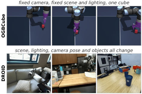
In diverse scenes, predictable background can dominate a prediction objective while action-relevant robot motion disappears. The paper adds inverse dynamics to make consecutive state representations informative about the action connecting them.
Environments and evaluation.
DROID plans are scored offline against expert end-effector paths using normalized discrete Fréchet distance. Zero corresponds to doing nothing, the expert path to 100%, and worse-than-static plans can score negative. This is a useful trajectory-quality proxy, not a direct manipulation success test.
Equation 7
(7)
Inverse dynamics loss avoids slow-feature collapse.
The inverse-dynamics head reconstructs actions from consecutive latent states. This constrains a joint temporal relationship that marginal Gaussian regularization cannot enforce. At higher levels, target macro-actions are detached so the encoder cannot satisfy reconstruction merely by co-adapting that target.
Equation 8
(8)
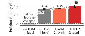
Fréchet fidelity (%) (b)(c)
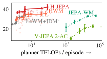
Figure 9: Scene diversity makes the inverse-dynamics loss necessary, and a second
level adds performance at a lower planner budget.(a) First frames of three Cube
and three DROID clips, showing scene variation across episodes.
(b)DROID at fps, Fréchet fidelity (%), showing the slow-feature-collapsed
LeWM, LeWM+IDM, then two hierarchies: HWM, whose level 2 is an identity encoder, and
H-JEPA, whose level 2 is learned. (c) The one-level and two-level models of
(b) swept over planner budgets, Fréchet fidelity against measured planner TFLOPs
per episode on a log axis, the bold line being the Pareto front. Two frozen-encoder world
models are shown for reference: they are public checkpoints, evaluated at their native
fps on the clips whose window fits at that rate, so their intervals span three
planner seeds. All other intervals are SE over three train seeds.
(a)
Hierarchical planning results.
SIGReg restores representation diversity, while inverse dynamics makes that diversity relevant to robot motion. With both present, a second hierarchy level improves the reported offline fidelity at lower planning budgets. The result does not establish successful closed-loop real-robot execution.
5 Related Work
H-JEPA builds on reward-free action-conditioned JEPAs, LeJEPA’s regularizer, and hierarchical planning. Its distinguishing combination is end-to-end prediction across several learned state spaces. It does not introduce temporal hierarchy, latent dynamics or inverse dynamics in isolation.
6 Conclusion
Separate timescales and representations can jointly support efficient planning. The demonstrated real-video extension depends on action supervision and an offline metric. Closed-loop physical-robot evaluation, action-free training, language goals and variable-duration abstractions remain future work.
Acknowledgments
The acknowledgments credit data, infrastructure and research contributions. They do not add an evaluation result or broaden the scope of the experiments.
Appendix A Notation
The full notation table distinguishes hierarchy levels, temporal strides, window sizes, action blocks and planning horizons. These conventions matter because an upper-level step can cover several lower-level transitions.
Table 2: Notation reference. Symbols are introduced in §2 unless the row names another section.
Level superscripts are always parenthesized, ; a bare subscript is a time index and
is a half-open range. Appendix-local symbols are defined where they are used.
Symbol
Description
Levels and indices
,
Hierarchy level index, ; level is the finest
Discrete time index, at the level’s own rate
Half-open slice: the indices
Observations, latents and actions
Image observation at time
Primitive action block for the transition
Level- latent state;
Action-conditioned autoregressive rollout at level
Optimized rollout produced by the level above; marks an optimized quantity
Level- action embedding (a macro-action for )
Optimized action sequence returned by the level- planner
Goal state at level , obtained by encoding the goal observation
Minibatch of level- embeddings, : rows of width
,
Sequences and timesteps of a minibatch of embeddings
,
Embedding width, and the number of data-parallel ranks (§K.3)
Learned components
State encoder at level ; pools a -step lower-level window
Action encoder at level ; pools an -step lower-level window for
,
Latent predictor and inverse-dynamics head at level
Autoregressive rollout operator induced by
Training objective
, ,
Total level- objective and its prediction and inverse-dynamics terms
FourRoomDistractors, AntMaze, Push-T, Cube and DROID differ in motion timescales, episode duration, scene diversity and available proprioception. These differences explain why one depth or objective does not behave identically across domains.
Appendix C Architecture and training
Architecture, optimization and dataset settings are separated between single-scene simulation and diverse DROID video. The distinction is central to interpreting the need for inverse dynamics.
C.1 Single-scene environments
The simulated hierarchies are trained jointly from scratch, so upper-level prediction losses can influence lower-level encoders. The flat LeWorldModel baseline uses the corresponding single-level recipe.
Data.
All compared depths use the same source data, but deeper hierarchies require longer within-episode clips. This reduces the effective transition coverage per epoch, especially on short Push-T episodes.
Table 3: Temporal layout of one training sample and the clips it leaves per
epoch. The minimum clip length is the shortest episode segment that yields one
training sample, in environment steps, including both endpoint observations. All H-JEPA
models use stride two and window one at every level above the first. A clip must
lie within one episode (the loader reserves environment steps per clip),
so the number of clips an epoch yields falls as the minimum clip length grows; parentheses give each count as a percentage of the LeWM count in the same
environment. Each clip supplies three teacher-forced transitions per level.
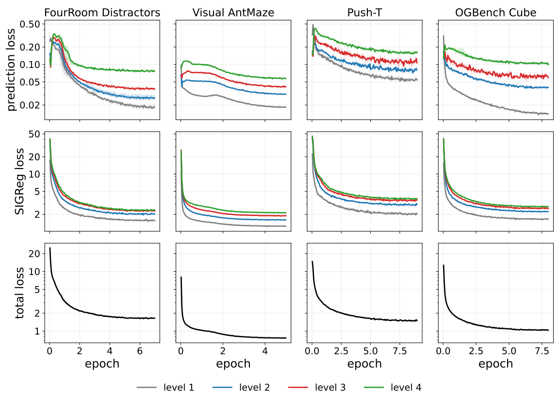
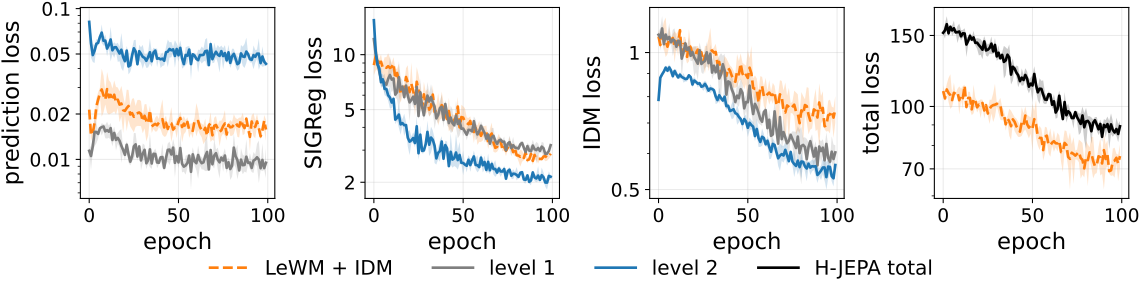
Early anti-collapse regularization spreads concentrated embeddings, so prediction loss can initially rise before declining. A near-zero prediction loss is not automatically desirable because a constant representation is trivial to predict. Both loss components and downstream probes are retained.
Figure 10: Per-level training losses of the four-level H-JEPA models and
of the DROID models. Top three rows: unweighted prediction loss and SIGReg
statistic of each level of the four-level models over training, and their
total training objective, the sum over levels of the prediction loss plus the
weighted SIGReg term. Every level of a model uses the same SIGReg weight
( on FourRoom, elsewhere), so the weighted curves differ from the
unweighted ones by a constant factor per environment. The seed band of the
total objective is narrower than its line.
Bottom row: unweighted prediction, SIGReg and inverse-dynamics losses of the
DROID flat LeWM+IDM (orange, dashed) and of both levels of the two-level H-JEPA
(solid) over their training epochs, and the total training objective, the sum
of all terms weighted as in Table 5 (level 1: SIGReg ,
IDM ; level 2: SIGReg , IDM ), summed over both levels for
H-JEPA. All curves are the mean over three training seeds with a min/max band,
on a log scale.
Architecture.
A projected vision-transformer token supplies the first representation, with added proprioceptive features where specified. Upper levels use compact encoders and action-conditioned causal predictors. Their distinct latent spaces are learned rather than manually assigned physical variables.
Training.
The recipe uses prediction and SIGReg losses at every level, finite random projections, AdamW and three training seeds. Equal epoch budgets do not imply equal usable data when temporal clip requirements differ.
Table 4: Per-environment architecture and training settings. Upper-level
predictor dimensions and H-JEPA epoch counts apply to every depth. H-JEPA models
are initialized independently of the LeWM baselines.
The implementation uses the stable-worldmodel and stable-pretraining libraries on the specified GPU hardware. Hardware-dependent timing should be separated from the reported planning-compute measure.
DROID training uses pixels and actions without proprioception and modifies data sampling and level weighting. Upper-level action embeddings also receive regularization to avoid collapsing macro-actions. These changes are part of the diverse-scene recipe, not an unchanged simulation model applied directly to real video.
Table 5: Training hyperparameters on DROID. Predictors are causal transformers, given as
width/depth. The grouping row
gives the shape of the tensor SIGReg tests: tests normality within each timestep,
over the sequences of the batch. The architecture and loss settings do not depend on
the training schedule, whether end-to-end or stagewise (§C.2); the
optimization block does, and reports the end-to-end headline runs. The peak learning rate is
the same at both levels, AdamW runs at , and the dataloader length caps the
iterations per epoch, which gives at this batch size.
World models are frozen before fitting probes and visualization decoders. These supervised diagnostic tools inspect learned information without supplying their targets to the world-model objective.
Probes.
Separate nonlinear probes predict each entity from each hierarchy level, reporting variance-normalized error. Low probe error measures recoverability under that probe family, not an identified causal factorization.
Decoder.
A lightweight decoder reconstructs images from a single latent for visualization. It does not turn the predictive training objective into pixel reconstruction.
Training.
Probe and decoder optimization is specified separately. Entity groups are classified by temporal frequency, so the analysis can distinguish retaining slow state from discarding faster detail rather than averaging all variables together.
Table 6: Probing data and probed entities per environment. Transition counts
are for fitting (train) and scoring (eval). Visual AntMaze is scored on one evaluation
set with equal numbers of explore and stitch episodes. On FourRoomDistractors and Visual
AntMaze, whose state separates into slow and fast entities
(Fig. 12), the entities are labeled accordingly. Entity
dimensions in parentheses.
Environment
transitions (train / eval)
Probed entities
FourRoomDistractors
k / k
slow: ego (2)
fast: distractor (2)
Visual AntMaze
k / k
slow: global (2)
fast: body state (27)
Push-T
k / k
agent (2), block (2),
block orientation (2), agent velocity (2)
OGBench Cube
k / k
cube position (3), cube orientation (6),
effector position (3), effector yaw (2), gripper (2),
arm joint positions (6), arm joint velocities (6)
Appendix E Planning evaluation
Evaluation tasks.
Held-out task pairs require navigation or manipulation over specified distances and horizons. Goals are images and, on AntMaze, accompanying proprioception. These controlled goal specifications differ from following free-form instructions.
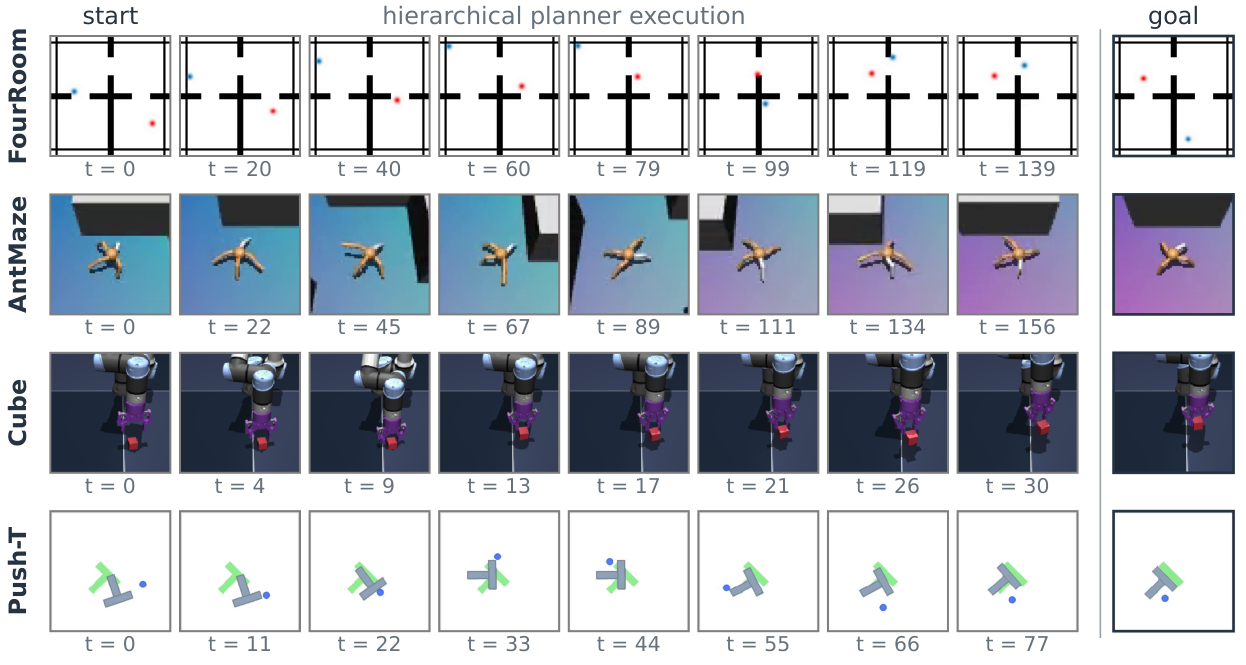
Figure 11: Successful hierarchical planner executions. Selected H-JEPA
executions on one evaluation task per environment, using three-level models for
FourRoom and AntMaze and two-level models for Cube and Push-T. These checkpoints
also appear in Fig. 6 (bottom); the recordings use their original
evaluation settings rather than the compute-selected sample counts. Each row
shows eight observations sampled uniformly in environment steps, followed by the
goal observation supplied to the planner. Rows end at first recorded success,
except Cube, which shows the full -step execution to include the completed
lift. Labels give elapsed environment steps.
Shared solver.
Each active level differentiates through candidate latent rollouts. Upper-level action search is calibrated to macro-actions observed during training because those latent actions lack native physical bounds. This anchoring limits unrealistic candidates but does not prove complete feasibility.
Replanning and horizons.
Models execute a fixed initial action chunk before replanning, with level-specific horizons that decrease during an episode. This keeps the comparison tied to the stated controller rather than assuming an open-loop plan is executed unchanged.
Reported settings.
Candidate budgets are selected on compute-sweep tasks and then evaluated on a separate task set. Depth comparisons vary candidate allocation while retaining the chosen learning rates and horizon settings.
Table 7: Planning settings for the simulated depth comparison.
: candidate sequences; : AdamW learning rate; : configured horizon
in predicted steps of that level, used by the schedule described above. Tuples
list levels from lowest to highest, except the H-JEPA learning-rate row, which
lists level one and the rate shared by all upper levels. Episode budgets are in
environment steps. Cube’s horizon-one upper solvers are skipped, so their listed
candidate counts are unused.
Table 8: Planning settings on DROID.
: candidate sequences; : AdamW
learning rate; : configured horizon in predicted steps of that level. Tuples list levels from lowest to highest. Every level runs
AdamW for at most iterations with early stopping when the best cost stalls; the
cross-level action cost is and the subgoal weight of
Eq. (6) is , for both two-level arms. Planning is open-loop: the whole level-1 plan is executed, so the commit
width equals the level-1 horizon. Each model keeps one and these settings at every
planner budget: the compute-Pareto of Fig. 9 varies only the number
of candidates, chosen independently per level for the two-level arms. The listed is the
operating point of each bar in Fig. 9.
Appendix F Temporal-frequency separation and selective abstraction
F.1 Frequency separation within a trajectory
An example AntMaze trajectory displays slow global motion and faster body dynamics at the sampling rate used for the spectral analysis. It illustrates the timescale statistic without replacing the aggregate multi-seed probe results.
Figure 12: Temporal-frequency separation and selective abstraction.(a) One AntMaze episode: normalized global position (red) and
body-state dimensions (blue) over level-1 frames (left), and cumulative
absolute normalized increments averaged across dimensions (right). Inverse
spectral centroids are about frames for position and for body state
( gap); body state accumulates roughly ten times more variation.
Including the omitted velocity dimensions leaves the frequency gap unchanged.
(b) Per-entity spectral centroids in cycles per level-1 frame (top, log
scale) and paired level-1 and level-2 probe macro NMSE (bottom). The left group
shows FourRoom, AntMaze and Humanoid; the right shows Push-T, OGBench Cube and
DROID. Probe heads are matched across levels within each environment and differ
across environments. Error bars are one SE over three training seeds. All entities
in an environment share the same level-2 configuration.
F.2 Per-entity probes across environments
Per-entity spectral centroids are paired with probe errors across environments. Larger temporal gaps coincide with selective loss of fast information at the next level; tasks without clear separation retain more entities together.
Appendix G Data specialization across levels
Stagewise training lets each hierarchy level use a different dataset, testing whether temporal data structure influences abstraction. This changes the training strategy as well as the data assigned to each level.
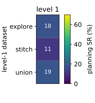
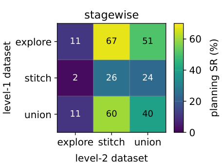
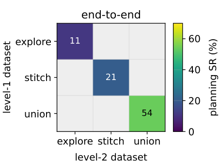
Figure 13: Planning with different training datasets on Visual AntMaze.
Planning success rate (GD online, mean over three seeds), using
explore, stitch, or their union for training.
Left: flat level-1 planning, with one model trained on each of the three
datasets. Middle: two-level hierarchical planning after stagewise
training, covering all nine combinations of level-1 (rows) and level-2
(columns) datasets. Right: two-level hierarchical planning after
end-to-end training, with both levels trained on the same dataset in
each run, giving only diagonal entries. Grey cells were not run.
The end-to-end runs are FLOP-matched to the stagewise ones.
Experimental setup.
AntMaze exploratory, stitched and combined trajectories are compared under stagewise and joint training. The controlled combinations distinguish a richer lower-level transition set from more coherent higher-level temporal patterns.
Matched data: a second level helps only when the data is temporally structured.
A second level helps more with temporally structured stitched trajectories than purely exploratory data in these experiments. Hierarchy cannot be assumed to create useful long-term abstraction from any arbitrary transition collection.
Appendix H Planning-cost ablations across environments
Cost-only ablations keep low-level dynamics fixed while changing the latent space used to score final states. This isolates representation geometry from splitting the temporal search.
FourRoom: gains from projected costs.
At least one upper-level cost improves FourRoom navigation, though the deepest cost is not always best. Overlapping error bars qualify small differences between projected costs.
Cube and Push-T: no clear gain from projected costs.
Cube and Push-T show no clear general benefit from upper-level cost projection, and some deep projections hurt. Their weak selective abstraction limits transferring the AntMaze cost-geometry explanation unchanged.
Table 9: Planning-cost ablations across environments.
Success (%, mean SE, three seeds), using the same protocol as
Table 1. Within each H-JEPA row, only the cost space varies
across the four level-1 planning columns; LeWM and hierarchical H-JEPA are
references. For FourRoom, bold marks the highest mean among cost spaces.
FourRoom gains from projected costs, while Cube and Push-T show no clear benefit.
Rank correlation compares latent-goal distance with progress along trajectories. It is a diagnostic of cost monotonicity in the chosen data, not a guarantee that every gradient direction leads to a feasible route.
Table 10: Prediction-cost monotonicity ( of
against time; higher is better; mean over three training
seeds, held-out episodes). L2 columns score each model’s level-2 encoding against the final
goal; subgoal scores a level-1 rollout, re-anchored to the true state at
each subgoal (bounded horizon), against the level-2 subgoals (per-segment).
Appendix J DROID: corpus, planning evaluation and offline metric
The appendix details real-video data selection and calibrates the offline trajectory metric against simulated task outcomes. Both are needed to bound the interpretation of DROID results.
J.1 Planning-evaluation protocol
Clips.
Evaluation clips are chosen to require non-greedy manipulation rather than trivial endpoint motion. Their selection and held-out separation are specified because a small curated set cannot support a broad deployment claim.
Frame rates.
Frame-rate choices define action blocks and the time span of each prediction. Results at one sampling rate should not be equated with the same model at another physical timescale.
Leak control.
The protocol separates evaluation data and training clips as described. This controls the reported test rather than establishing absence of every possible pretraining overlap.
Task and action space.
Planning acts in the end-effector delta-pose space and compares with recorded expert paths. The action convention determines what the offline fidelity score measures.
J.2 The Fréchet fidelity offline metric
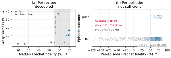
Fréchet fidelity normalizes path discrepancy by a do-nothing baseline. Calibration shows that an expert-like path can be necessary for success while still failing to complete a task, and can rank partial progress more smoothly than binary outcomes.
Against a binary outcome it is a necessary condition.
Following much of the expert path does not ensure final completion. A high offline score can therefore be a necessary but insufficient indicator under the tested tasks.
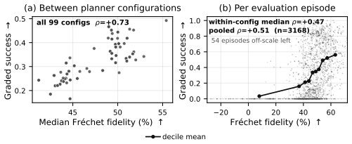
Against a continuous outcome it ranks progress.
Against a continuous progress measure, the metric can order partial improvements. Its calibration is empirical and tied to the selected simulation and trajectory conventions.
Figure 14: On OGBench Cube, where the outcome is observable, Fréchet fidelity
separates the episodes that can succeed from those that cannot, but not the ones that do. One frozen checkpoint,
configuration groups planner seeds episodes. (a) One
point per planner configuration; in the shaded band the flat and hierarchical planners have
equal offline fidelity and opposite grasp outcomes. (b) Every episode: none succeeds
below a fidelity threshold, and most above it still fail.
Figure 15: Against a continuous outcome the same offline metric ranks degree of
progress. RoboCasa CloseDrawer, one frozen checkpoint, planner configurations
held-out episodes, budget steps; the configurations are varied to spread
the outcomes, not tuned for task performance. is Fréchet fidelity, computed
exactly as on DROID; is graded drawer-closure success, a continuous outcome DROID
cannot report. (a) One point per planner configuration, median fidelity against mean
graded success. (b) Every episode, with the mean of each fidelity decile joined. The
claim rests on the within-configuration rank correlation, which holds episode
difficulty and planner settings fixed; the pooled and between-configuration values are
inflated by a between-configuration mean shift.
J.3 Decoded plans
Decoded plans expose motion and errors hidden by one scalar fidelity score. They visualize imagined trajectories under planned actions, not frames obtained from executing those actions on a physical robot.
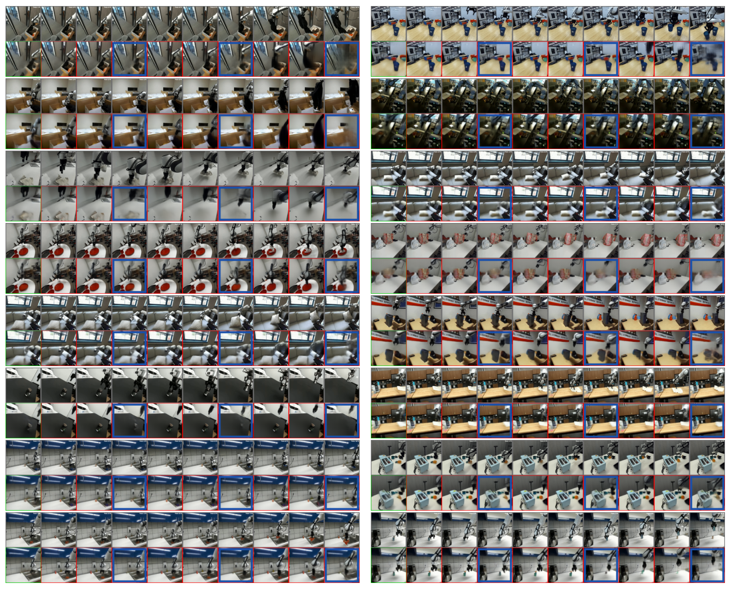
Figure 16: What the DROID planner imagines, on every clip of the evaluation set.
Two-level stagewise model, held-out, training seed 1; all clips ordered best
to worst by Fréchet fidelity, down the left column then the right, down
to at the zero-action floor. Each clip is two strips: above, the logged expert clip;
below, the decoded plan, which is the level-1 rollout under the planner’s committed commands
with the level-2 macro-plan interleaved into it at every third column (temporal stride
), ringed in blue. Columns are timesteps. The leftmost is the context frame the planner
is given (green); the rest are imagined (red), and blur along the rollout, which is the
decoder’s fidelity limit and not a planning failure.
J.4 The re-encoded training corpus
A re-encoded DROID copy reduces decoding and storage overhead while retaining frames and timestamps. The documented preprocessing is part of reproducing the training data; it should not be confused with a new model contribution.
J.5 Future work
Joint multi-camera encoding, wrist views and action-free training remain open extensions. Removing action labels would also remove the inverse-dynamics signal used to prevent the demonstrated diverse-scene failure.
Appendix K Anti-collapse: SIGReg, inverse dynamics and detachment
SIGReg tests the marginal distribution of representations; inverse dynamics tests temporal action information. Target detachment changes gradient flow. Their roles are separated because a high-rank distribution alone need not represent controllable motion.
Equation 9
(9)
K.1 What SIGReg, IDM and detachment each contribute
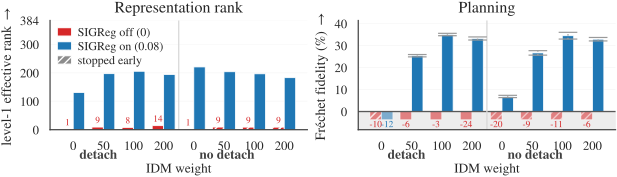
The coefficient grid shows that SIGReg can maintain rank while planning remains poor without sufficient inverse-dynamics weight. Detachment is not a general replacement for either information diversity or action relevance.
Figure 17: SIGReg restores representation rank; the inverse-dynamics term is what
turns rank into planning fidelity. Full grid around the level-1 DROID configuration of
table5: SIGRegIDM weight
prediction-target detachment, cells, one training seed each, read at epoch
. Five SIGReg-off cells (hatched) were stopped once collapsed and are read at their
last epoch.
Left: level-1 effective rank [25] of the CLS embedding, max .
Right: Fréchet fidelity on the 16-clip set; the grey band
holds sub-floor cells, drawn as fixed-depth stubs annotated with their true value. Each
planning bar is the mean over planner seeds , and of one trained model, and its
error bar is the standard error (SE) over those three planner seeds.
K.2 Cross-validating the SIGReg and inverse-dynamics coefficients
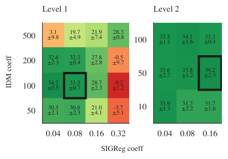
The two loss coefficients are tuned jointly, and the next level is tuned after freezing the previous stage in this analysis. One coefficient’s effect cannot be interpreted independently of the other’s scale.
Figure 18: The SIGReg and inverse-dynamics coefficients are chosen jointly, once per
level.DROID at fps; Fréchet fidelity (%, higher is better), mean and standard
error over three training seeds, each averaged over three planner seeds. Left, the
level-1 grid on single-level models; right, the level-2 grid on stagewise models with
level 1 frozen. Both use the gradient-based planner of our headline results, and share one
color scale. The heavy outline marks the coefficients we keep; at level 1 they lie within one
standard error of the best cell.
The normality statistic is not a sum of per-example terms. The implementation aggregates empirical characteristic functions across devices before evaluating the statistic, maintaining consistency for a fixed global batch when the data is sharded differently.
Table 11: Our distributed SIGReg is exactly invariant to how a fixed total batch is
sharded; a single-GPU implementation is not. One fixed Gaussian matrix (, ,
directions) sharded contiguously across ranks in float64. The reference is the SIGReg released with LeWM [53], formula-identical to ours but with its prefactor set by the local batch and no collective; its code documents itself as single-GPU. The data follow the target, so its drift is launch topology, not signal.
Appendix L Slow-feature collapse in joint-embedding predictive objectives
The theory distinguishes avoiding a constant vector from avoiding a representation that is constant within each episode. Background-only embeddings can be diverse across episodes and perfectly predictable while useless for controlling the moving agent.
L.1 Three kinds of content in a sequence of observations
The analysis separates episode-constant background, action-driven foreground and other changing content. It defines slow-feature collapse through what the encoder retains within an episode, rather than through global covariance alone.
Equation 10
(10)
L.2 Where the latent variance goes
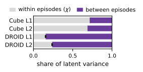
A variance decomposition compares within- and between-episode variation. Diverse scenes can consume most latent capacity in scene identity even though a same-episode difference cancels a constant offset. Cancellation alone does not restore the omitted robot information.
Figure 19: Scene diversity sends
latent variance between episodes. Within-episode (the slow-feature degree of
Definition1) and between-episode shares of the latent variance.
Bars are 1 standard error (SE) over three training seeds.
L.3 No regularizer on the marginal law can exclude it
With an atomless readable background and a regularizer depending only on the single-embedding marginal law, the construction can match the regularizer’s target while encoding only background. This is an existence result under explicit assumptions, not a statement that every trained model must reach that solution.
L.4 The objective selects by predictability, and the collapse is an optimum
The optimal predictor’s residual risk is bounded by unpredictable latent variation. Thus a perfectly predictable background representation can be globally attractive under the modeled objective. The characterization clarifies when preserving foreground introduces irreducible prediction cost.
Experiments of Sobal et al. [72] .
Earlier dot experiments are interpreted using the background/controlled/random taxonomy. These are supporting examples of the proposed mechanism, not independent proof that every nuisance variable behaves the same way.
L.5 Pooling time into the sample axis: a real but small barrier
Pooling time into the batch makes repeated within-episode embeddings visible to a finite-sample normality test. The resulting barrier can be real but small, so a nonzero SIGReg penalty alone does not reliably prevent background-only representations.
Equation 11
(11)
Table 12: Training without the inverse-dynamics term: the SIGReg
ladder (top) and time repulsion at its largest coefficient (middle). Level-1 models at
fps, , three train seeds, epochs. These runs feed SIGReg the flattened
tensor, one normality test over all embeddings of the minibatch, which places
time in the sample axis, so they carry the of Proposition2;
the barrier is what the ladder probes. “Onset” is the first epoch at which Fréchet fidelity (Eq. (7)) drops clearly below the zero-action floor, the next column the epoch at which the predictor’s action sensitivity first falls below (seed spread epochs). Best fidelity is the highest before turning over; final fidelity and sensitivity are read over epochs –; is Eq. (10) on the final checkpoint (one seed for the repulsion runs, three for the IDM-on row). Ladder rows carry no terminal value (at most two seeds reach epoch ).
L.6 Time repulsion: a barrier that needs no action labels
Rewarding temporal change uses pairwise information and can oppose episode-constant collapse without action labels. It can also reward irrelevant fast distractors, so it is not interchangeable with a control-aware inverse-dynamics objective.
L.7 The inverse-dynamics term is a barrier of a different order
If representations reveal only background, action reconstruction retains a dataset-dependent error floor. This provides a qualitatively different barrier from marginal regularization, assuming actions are not already determined by background identity.
Equation 12
(12)
Appendix M Extended related work
M.1 World models and planning
The extended survey places predictive latent models among generative simulators and model-based policy-learning methods. These approaches differ in rewards, reconstruction, pretraining and deployment-time search.
Contrastive negatives, architectural asymmetry, covariance regularization and distribution matching address constant collapse differently. The paper’s slow-feature analysis adds a separate issue: useful temporal content can disappear even when global distributional diversity survives.
M.3 Hierarchical World Models
Earlier hierarchical video and latent models use different timescales and sometimes reconstruction. H-JEPA combines a learned representation hierarchy with action-conditioned prediction and explicit planning, rather than claiming hierarchy itself is new.
M.4 Hierarchical control
Hierarchical policies and classical hierarchical model-predictive controllers organize decisions across timescales. H-JEPA learns predictive abstractions from offline observations and actions, then searches through them; that distinction limits comparisons with reward-trained policies and known-dynamics controllers.
Table 13: Model-based hierarchical control methods along four axes that define H-JEPA.Pixels: operates from high-dimensional visual observations rather than a
low-dimensional state.
Task-agnostic: reward-free training with no task signal; the task objective
(a goal or a planning cost) is defined only at test time.
Reconstruction Free: learns representations and dynamics with no reconstruction
objective, predicting latent targets rather than decoding observations.
Hierarchy of learned latent spaces: a stack
of distinct latent spaces, each a coarser abstraction of the one below that
discards detail (vs. a single/shared space, parallel spaces, or a hierarchy of
decisions only). ✓ yes, ✗ no, partial. H-JEPA is the only method satisfying all four;
HWM, our baseline, differs on exactly one axis.
[1]
Mahmoud Assran, Quentin Duval, Ishan Misra, Piotr Bojanowski, Pascal Vincent,
Michael Rabbat, Yann LeCun, and Nicolas Ballas.
Self-supervised learning from images with a joint-embedding
predictive architecture.
In IEEE/CVF Conference on Computer Vision and Pattern
Recognition (CVPR), 2023.
arXiv:2301.08243.
[3]
Christopher Baldassano, Janice Chen, Asieh Zadbood, Jonathan W. Pillow, Uri
Hasson, and Kenneth A. Norman.
Discovering event structure in continuous narrative perception and
memory.
Neuron, 95(3):709–721, 2017.
[4]
Federico Baldassarre, Marc Szafraniec, Basile Terver, Vasil Khalidov, Francisco
Massa, Yann LeCun, Patrick Labatut, Maximilian Seitzer, and Piotr Bojanowski.
Back to the features: Dino as a foundation for video world models,
2025.
URLhttps://arxiv.org/abs/2507.19468.
[5]
Randall Balestriero and Yann LeCun.
Learning by reconstruction produces uninformative features for
perception, 2024.
URLhttps://arxiv.org/abs/2402.11337.
[6]
Randall Balestriero and Yann LeCun.
Lejepa: Provable and scalable self-supervised learning without the
heuristics.
https://arxiv.org/abs/2511.08544, 2025.
[7]
Amir Bar, Gaoyue Zhou, Danny Tran, Trevor Darrell, and Yann LeCun.
Navigation world models.
In Proceedings of the IEEE/CVF Conference on Computer Vision
and Pattern Recognition (CVPR), pp. 15791–15801, June 2025.
[8]
Adrien Bardes, Jean Ponce, and Yann LeCun.
VICReg: Variance-invariance-covariance regularization for
self-supervised learning.
In International Conference on Learning Representations
(ICLR), 2022.
arXiv:2105.04906.
[10]
Tim Brooks, Bill Peebles, Connor Holmes, Will DePue, Yufei Guo, Li Jing, David
Schnurr, Joe Taylor, Troy Luhman, Eric Luhman, Clarence Ng, Ricky Wang, and
Aditya Ramesh.
Video generation models as world simulators.
OpenAI technical report,
https://openai.com/index/video-generation-models-as-world-simulators/,
2024.
[11]
Jake Bruce, Michael D. Dennis, Ashley Edwards, Jack Parker-Holder, Yuge Shi,
Edward Hughes, Matthew Lai, Aditi Mavalankar, Richie Steigerwald, Chris Apps,
Yusuf Aytar, Sarah Bechtle, Feryal Behbahani, Stephanie Chan, Nicolas Heess,
Lucy Gonzalez, Simon Osindero, Sherjil Ozair, Scott Reed, Jingwei Zhang,
Konrad Zolna, Jeff Clune, Nando de Freitas, Satinder Singh, and Tim
Rocktäschel.
Genie: Generative interactive environments.
In International Conference on Machine Learning (ICML), 2024.
arXiv:2402.15391.
[12]
Mathilde Caron, Hugo Touvron, Ishan Misra, Hervé Jégou, Julien Mairal,
Piotr Bojanowski, and Armand Joulin.
Emerging properties in self-supervised vision transformers.
In IEEE/CVF International Conference on Computer Vision
(ICCV), 2021.
arXiv:2104.14294.
[13]
Ting Chen, Simon Kornblith, Mohammad Norouzi, and Geoffrey Hinton.
A simple framework for contrastive learning of visual
representations.
In International Conference on Machine Learning (ICML), 2020.
arXiv:2002.05709.
[15]
Cheng Chi, Siyuan Feng, Yilun Du, Zhenjia Xu, Eric Cousineau, Benjamin
Burchfiel, and Shuran Song.
Diffusion policy: Visuomotor policy learning via action diffusion.
In Robotics: Science and Systems (RSS), 2023.
arXiv:2303.04137.
[16]
Andy Clark.
Whatever next? predictive brains, situated agents, and the future of
cognitive science.
Behavioral and Brain Sciences, 36(3):181–204, 2013.
[19]
Yilun Du, Mengjiao Yang, Bo Dai, Hanjun Dai, Ofir Nachum, Joshua B. Tenenbaum,
Dale Schuurmans, and Pieter Abbeel.
Learning universal policies via text-guided video generation.
In Advances in Neural Information Processing Systems
(NeurIPS), 2023.
arXiv:2302.00111.
[20]
Frederik Ebert, Chelsea Finn, Sudeep Dasari, Annie Xie, Alex Lee, and Sergey
Levine.
Visual foresight: Model-based deep reinforcement learning for
vision-based robotic control.
arXiv preprint arXiv:1812.00568, 2018.
[23]
Kuan Fang, Yuke Zhu, Animesh Garg, Silvio Savarese, and Li Fei-Fei.
Dynamics learning with cascaded variational inference for multi-step
manipulation.
In Conference on Robot Learning (CoRL), 2019.
arXiv:1910.13395.
[24]
Chelsea Finn and Sergey Levine.
Deep visual foresight for planning robot motion.
In IEEE International Conference on Robotics and Automation
(ICRA), pp. 2786–2793, 2017.
arXiv:1610.00696.
[25]
Quentin Garrido, Randall Balestriero, Laurent Najman, and Yann LeCun.
Rankme: assessing the downstream performance of pretrained
self-supervised representations by their rank.
In Proceedings of the 40th International Conference on Machine
Learning, ICML’23. JMLR.org, 2023.
[26]
Jean-Bastien Grill, Florian Strub, Florent Altché, Corentin Tallec,
Pierre H. Richemond, Elena Buchatskaya, Carl Doersch, Bernardo Avila Pires,
Zhaohan Daniel Guo, Mohammad Gheshlaghi Azar, Bilal Piot, Koray Kavukcuoglu,
Rémi Munos, and Michal Valko.
Bootstrap your own latent: A new approach to self-supervised
learning.
In Advances in Neural Information Processing Systems
(NeurIPS), 2020.
arXiv:2006.07733.
[27]
Christian Gumbsch, Noor Sajid, Georg Martius, and Martin V. Butz.
Learning hierarchical world models with adaptive temporal
abstractions from discrete latent dynamics.
In International Conference on Learning Representations
(ICLR), 2024.
[29]
David Ha and Jürgen Schmidhuber.
Recurrent world models facilitate policy evolution.
In Advances in Neural Information Processing Systems
(NeurIPS), 2018.
arXiv:1803.10122 (“World Models”).
[30]
Danijar Hafner, Timothy Lillicrap, Ian Fischer, Ruben Villegas, David Ha,
Honglak Lee, and James Davidson.
Learning latent dynamics for planning from pixels.
In International Conference on Machine Learning (ICML), 2019.
arXiv:1811.04551.
[31]
Danijar Hafner, Timothy Lillicrap, Jimmy Ba, and Mohammad Norouzi.
Dream to control: Learning behaviors by latent imagination.
In International Conference on Learning Representations
(ICLR), 2020.
arXiv:1912.01603.
[32]
Danijar Hafner, Kuang-Huei Lee, Ian Fischer, and Pieter Abbeel.
Deep hierarchical planning from pixels.
In Advances in Neural Information Processing Systems
(NeurIPS), 2022.
arXiv:2206.04114.
[33]
Danijar Hafner, Jurgis Pasukonis, Jimmy Ba, and Timothy Lillicrap.
Mastering diverse domains through world models.
arXiv preprint arXiv:2301.04104, 2023.
Published in Nature 640:647–653, 2025.
[34]
Nicklas Hansen, Hao Su, and Xiaolong Wang.
Temporal difference learning for model predictive control.
In International Conference on Machine Learning (ICML), 2022.
arXiv:2203.04955.
[35]
Nicklas Hansen, Hao Su, and Xiaolong Wang.
TD-MPC2: Scalable, robust world models for continuous control.
In International Conference on Learning Representations
(ICLR), 2024.
arXiv:2310.16828.
[36]
Nicklas Hansen, Jyothir S V, Vlad Sobal, Yann LeCun, Xiaolong Wang, and Hao Su.
Hierarchical world models as visual whole-body humanoid controllers.
In International Conference on Learning Representations
(ICLR), 2025.
arXiv:2405.18418.
[37]
Uri Hasson, Eunice Yang, Ignacio Vallines, David J. Heeger, and Nava Rubin.
A hierarchy of temporal receptive windows in human cortex.
Journal of Neuroscience, 28(10):2539–2550, 2008.
[40]
Petr Ivashkov, Randall Balestriero, and Bernhard Schölkopf.
Sensorimotor world models: Perception for action via inverse
dynamics, 2026.
URLhttps://arxiv.org/abs/2606.20104.
[41]
Michael Janner, Yilun Du, Joshua B. Tenenbaum, and Sergey Levine.
Planning with diffusion for flexible behavior synthesis.
In International Conference on Machine Learning (ICML), 2022.
arXiv:2205.09991.
[42]
Alexander Khazatsky, Karl Pertsch, Suraj Nair, Ashwin Balakrishna, Sudeep
Dasari, Siddharth Karamcheti, Soroush Nasiriany, Mohan Kumar Srirama,
Lawrence Yunliang Chen, Kirsty Ellis, et al.
Droid: A large-scale in-the-wild robot manipulation dataset.
In Robotics: Science and Systems (RSS), 2024.
[43]
Stefan J. Kiebel, Jean Daunizeau, and Karl J. Friston.
A hierarchy of time-scales and the brain.
PLoS Computational Biology, 4(11):e1000209, 2008.
[44]
Taesup Kim, Sungjin Ahn, and Yoshua Bengio.
Variational temporal abstraction.
In Advances in Neural Information Processing Systems
(NeurIPS), 2019.
arXiv:1910.00775.
[45]
Markus Kögel, Mohamed Ibrahim, Christian Kallies, and Rolf Findeisen.
Safe hierarchical model predictive control and planning for
autonomous systems.
International Journal of Robust and Nonlinear Control, 2023.
arXiv:2203.14269.
[46]
Yilun Kuang, Yash Dagade, Quentin Le Lidec, Lucas Maes, Randall Balestriero,
and Yann LeCun.
LpWM: A case for sparse representations in world models.
arXiv preprint arXiv:2608.22764, 2026a.
[47]
Yilun Kuang, Yash Dagade, Tim G. J. Rudner, Randall Balestriero, and Yann
LeCun.
Rectified lpjepa: Joint-embedding predictive architectures with
sparse and maximum-entropy representations, 2026b.
URLhttps://arxiv.org/abs/2602.01456.
[48]
Alex Lamb, Riashat Islam, Yonathan Efroni, Aniket Rajiv Didolkar, Dipendra
Misra, Dylan J Foster, Lekan P Molu, Rajan Chari, Akshay Krishnamurthy, and
John Langford.
Guaranteed discovery of control-endogenous latent states with
multi-step inverse models.
Transactions on Machine Learning Research, 2023.
ISSN 2835-8856.
URLhttps://openreview.net/forum?id=TNocbXm5MZ.
[52]
Etai Littwin, Omid Saremi, Madhu Advani, Vimal Thilak, Preetum Nakkiran, Chen
Huang, and Joshua M. Susskind.
How JEPA avoids noisy features: The implicit bias of deep linear
self distillation networks.
In The Thirty-eighth Annual Conference on Neural Information
Processing Systems, 2024.
URLhttps://openreview.net/forum?id=ez7w0Ss4g9.
[54]
Vincent Micheli, Eloi Alonso, and François Fleuret.
Transformers are sample-efficient world models.
In International Conference on Learning Representations
(ICLR), 2023.
arXiv:2209.00588.
[55]
Ramy Mounir, Sujal Vijayaraghavan, and Sudeep Sarkar.
STREAMER: Streaming representation learning and event segmentation
in a hierarchical manner.
In Advances in Neural Information Processing Systems
(NeurIPS), 2023.
[56]
John D. Murray, Alberto Bernacchia, David J. Freedman, Ranulfo Romo,
Jonathan D. Wallis, Xinying Cai, Camillo Padoa-Schioppa, Tatiana Pasternak,
Hyojung Seo, Daeyeol Lee, and Xiao-Jing Wang.
A hierarchy of intrinsic timescales across primate cortex.
Nature Neuroscience, 17(12):1661–1663,
2014.
[57]
Ofir Nachum, Shixiang Gu, Honglak Lee, and Sergey Levine.
Data-efficient hierarchical reinforcement learning.
In Advances in Neural Information Processing Systems
(NeurIPS), 2018.
arXiv:1805.08296.
[59]
Nilaksh, Saurav Jha, Artem Zholus, and Sarath Chandar.
Reconstruction or semantics? what makes a latent space useful for
robotic world models, 2026.
URLhttps://arxiv.org/abs/2605.06388.
[61]NVIDIA, :, Mayank Mittal, Pascal Roth, James Tigue, Antoine Richard, Octi
Zhang, Peter Du, Antonio Serrano-Muñoz, Xinjie Yao, René Zurbrügg, Nikita
Rudin, Lukasz Wawrzyniak, Milad Rakhsha, Alain Denzler, Eric Heiden, Ales
Borovicka, Ossama Ahmed, Iretiayo Akinola, Abrar Anwar, Mark T. Carlson,
Ji Yuan Feng, Animesh Garg, Renato Gasoto, Lionel Gulich, Yijie Guo,
M. Gussert, Alex Hansen, Mihir Kulkarni, Chenran Li, Wei Liu, Viktor
Makoviychuk, Grzegorz Malczyk, Hammad Mazhar, Masoud Moghani, Adithyavairavan
Murali, Michael Noseworthy, Alexander Poddubny, Nathan Ratliff, Welf Rehberg,
Clemens Schwarke, Ritvik Singh, James Latham Smith, Bingjie Tang, Ruchik
Thaker, Matthew Trepte, Karl Van Wyk, Fangzhou Yu, Alex Millane, Vikram
Ramasamy, Remo Steiner, Sangeeta Subramanian, Clemens Volk, CY Chen, Neel
Jawale, Ashwin Varghese Kuruttukulam, Michael A. Lin, Ajay Mandlekar, Karsten
Patzwaldt, John Welsh, Huihua Zhao, Fatima Anes, Jean-Francois Lafleche,
Nicolas Moënne-Loccoz, Soowan Park, Rob Stepinski, Dirk Van Gelder, Chris
Amevor, Jan Carius, Jumyung Chang, Anka He Chen, Pablo de Heras Ciechomski,
Gilles Daviet, Mohammad Mohajerani, Julia von Muralt, Viktor Reutskyy,
Michael Sauter, Simon Schirm, Eric L. Shi, Pierre Terdiman, Kenny Vilella,
Tobias Widmer, Gordon Yeoman, Tiffany Chen, Sergey Grizan, Cathy Li, Lotus
Li, Connor Smith, Rafael Wiltz, Kostas Alexis, Yan Chang, David Chu,
Linxi "Jim" Fan, Farbod Farshidian, Ankur Handa, Spencer Huang, Marco Hutter,
Yashraj Narang, Soha Pouya, Shiwei Sheng, Yuke Zhu, Miles Macklin, Adam
Moravanszky, Philipp Reist, Yunrong Guo, David Hoeller, and Gavriel State.
Isaac lab: A gpu-accelerated simulation framework for multi-modal
robot learning, 2025.
URLhttps://arxiv.org/abs/2511.04831.
[62]
Artidoro Pagnoni, Ram Pasunuru, Pedro Rodriguez, John Nguyen, Benjamin Muller,
Margaret Li, Chunting Zhou, Lili Yu, Jason Weston, Luke Zettlemoyer, Gargi
Ghosh, Mike Lewis, Ari Holtzman, and Srinivasan Iyer.
Byte latent transformer: Patches scale better than tokens.
arXiv preprint arXiv:2412.09871, 2024.
[63]
Seohong Park, Kevin Frans, Benjamin Eysenbach, and Sergey Levine.
OGBench: Benchmarking offline goal-conditioned RL.
In International Conference on Learning Representations
(ICLR), 2025.
arXiv:2410.20092.
[64]
Deepak Pathak, Pulkit Agrawal, Alexei A. Efros, and Trevor Darrell.
Curiosity-driven exploration by self-supervised prediction.
In Proceedings of the 34th International Conference on Machine
Learning (ICML), volume 70 of Proceedings of Machine Learning
Research, pp. 2778–2787. PMLR, 2017.
arXiv:1705.05363.
[65]
Karl Pertsch, Oleh Rybkin, Frederik Ebert, Shenghao Zhou, Dinesh Jayaraman,
Chelsea Finn, and Sergey Levine.
Long-horizon visual planning with goal-conditioned hierarchical
predictors.
In Advances in Neural Information Processing Systems
(NeurIPS), 2020.
arXiv:2006.13205.
[66]
Jean Ponce, Basile Terver, Martial Hebert, and Michael Arbel.
Dual perspectives on non-contrastive self-supervised learning.
In The Fourteenth International Conference on Learning
Representations, 2026.
URLhttps://openreview.net/forum?id=f5MC1G6XhB.
[67]
Rajesh P. N. Rao and Dana H. Ballard.
Predictive coding in the visual cortex: A functional interpretation
of some extra-classical receptive-field effects.
Nature Neuroscience, 2(1):79–87, 1999.
[68]
Vaibhav Saxena, Jimmy Ba, and Danijar Hafner.
Clockwork variational autoencoders.
In Advances in Neural Information Processing Systems
(NeurIPS), 2021.
arXiv:2102.09532.
[69]
Robin Schiewer, Anand Subramoney, and Laurenz Wiskott.
Exploring the limits of hierarchical world models in reinforcement
learning.
Scientific Reports, 14, 2024.
arXiv:2406.00483; DOI 10.1038/s41598-024-76719-w.
[70]
Julian Schrittwieser, Ioannis Antonoglou, Thomas Hubert, Karen Simonyan,
Laurent Sifre, Simon Schmitt, Arthur Guez, Edward Lockhart, Demis Hassabis,
Thore Graepel, Timothy Lillicrap, and David Silver.
Mastering atari, go, chess and shogi by planning with a learned
model.
Nature, 588(7839):604–609, 2020.
arXiv:1911.08265.
[71]
Chang Shi, Tim Pearce, Manan Tomar, Siddhartha Sen, and John Langford.
Hierarchical latent prediction for language models.
arXiv preprint arXiv:2608.05806, 2026.
[73]
Vlad Sobal, Wancong Zhang, Kyunghyun Cho, Randall Balestriero, Tim G. J.
Rudner, and Yann LeCun.
Learning from reward-free offline data: A case for planning with
latent dynamics models.
arXiv preprint arXiv:2502.14819, 2025.
[74]
Richard S. Sutton and Andrew G. Barto.
An adaptive network that constructs and uses an internal model of its
world.
Cognition and Brain Theory, pp. 217–246, 1981.
[75]
Richard S. Sutton, Doina Precup, and Satinder Singh.
Between MDPs and semi-MDPs: A framework for temporal abstraction
in reinforcement learning.
Artificial Intelligence, 112(1-2):181–211, 1999.
[76]
Yunhao Tang, Zhaohan Daniel Guo, Pierre Harvey Richemond, Bernardo
Ávila Pires, Yash Chandak, Rémi Munos, Mark Rowland,
Mohammad Gheshlaghi Azar, Charline Le Lan, Clare Lyle, András György,
Shantanu Thakoor, Will Dabney, Bilal Piot, Daniele Calandriello, and Michal
Valko.
Understanding self-predictive learning for reinforcement learning.
In Proceedings of the 40th International Conference on Machine
Learning (ICML), volume 202 of Proceedings of Machine Learning
Research. PMLR, 2023.
arXiv:2212.03319.
[77]
Basile Terver, Randall Balestriero, Megi Dervishi, David Fan, Quentin Garrido,
Tushar Nagarajan, Koustuv Sinha, Wancong Zhang, Mike Rabbat, Yann LeCun, and
Amir Bar.
A lightweight library for energy-based joint-embedding predictive
architectures.
https://arxiv.org/abs/2602.03604, 2026a.
[78]
Basile Terver, Tsung-Yen Yang, Jean Ponce, Adrien Bardes, and Yann LeCun.
What drives success in physical planning with joint-embedding
predictive world models?
Transactions on Machine Learning Research (TMLR),
2026b.
arXiv:2512.24497.
[80]
Alexander Sasha Vezhnevets, Simon Osindero, Tom Schaul, Nicolas Heess, Max
Jaderberg, David Silver, and Koray Kavukcuoglu.
FeUdal networks for hierarchical reinforcement learning.
In International Conference on Machine Learning (ICML), 2017.
arXiv:1703.01161.
[81]
Tongzhou Wang, Simon Du, Antonio Torralba, Phillip Isola, Amy Zhang, and
Yuandong Tian.
Denoised MDPs: Learning world models better than the world itself.
In Kamalika Chaudhuri, Stefanie Jegelka, Le Song, Csaba Szepesvari,
Gang Niu, and Sivan Sabato (eds.), Proceedings of the 39th
International Conference on Machine Learning, volume 162 of
Proceedings of Machine Learning Research, pp. 22591–22612. PMLR,
17–23 Jul 2022.
URLhttps://proceedings.mlr.press/v162/wang22c.html.
[84]
Manuel Watter, Jost Tobias Springenberg, Joschka Boedecker, and Martin
Riedmiller.
Embed to control: A locally linear latent dynamics model for control
from raw images.
In Advances in Neural Information Processing Systems
(NeurIPS), 2015.
arXiv:1506.07365.
[86]
Björn Weghenkel and Laurenz Wiskott.
Slowness as a proxy for temporal predictability: An empirical
comparison.
Neural Computation, 30(5):1151–1179, 05
2018.
ISSN 0899-7667.
doi: 10.1162/neco_a_01070.
URLhttps://doi.org/10.1162/neco_a_01070.
[88]
Jialong Wu, Shaofeng Yin, Ningya Feng, Xu He, Dong Li, Jianye Hao, and
Mingsheng Long.
iVideoGPT: Interactive videogpts are scalable world models.
In Advances in Neural Information Processing Systems
(NeurIPS), 2024.
arXiv:2405.15223.
[89]
Philipp Wu, Alejandro Escontrela, Danijar Hafner, Ken Goldberg, and Pieter
Abbeel.
Daydreamer: World models for physical robot learning.
In Conference on Robot Learning (CoRL), 2022.
arXiv:2206.14176.
[90]
Mengjiao Yang, Yilun Du, Kamyar Ghasemipour, Jonathan Tompson, Dale Schuurmans,
and Pieter Abbeel.
Learning interactive real-world simulators.
In International Conference on Learning Representations
(ICLR), 2024.
arXiv:2310.06114.
[91]
Jure Zbontar, Li Jing, Ishan Misra, Yann LeCun, and Stéphane Deny.
Barlow twins: Self-supervised learning via redundancy reduction.
In International Conference on Machine Learning (ICML), 2021.
arXiv:2103.03230.
[93]
Gaoyue Zhou, Hengkai Pan, Yann LeCun, and Lerrel Pinto.
DINO-WM: World models on pre-trained visual features enable
zero-shot planning.
In International Conference on Machine Learning (ICML), 2025.
arXiv:2411.04983.
 (b)
 (c)
 (a)