Overview
This edition follows the 25-page arXiv v2 dated 2 November 2026, preserving four numbered figures with all panels, three numbered tables, the algorithm, twelve displayed formulas, seven printed prompt blocks and 28 references. Bayesian active learning chooses contrasts between formal task hypotheses; language models still propose, interpret and score those hypotheses. The main “human-approval” evaluation uses automated ground-truth verification. Human participants answer questions about assigned tasks rather than composing goals or approving plans. Formal planning verifies the inferred specification, not whether that specification is the person’s true intent.
At a glance
The system maintains a probabilistic utility model over candidate temporal-logic tasks and asks questions intended to reduce uncertainty. A grammar-constrained latent space permits challengers beyond the language model’s initial proposals. Tested across two simulated domains, a constrained human study and two physical sites, it generally improves task satisfaction and dialogue efficiency over direct language-model clarification. Its evidence remains conditional on known predicates, accurate scene representations and the evaluation protocol.
1 Introduction
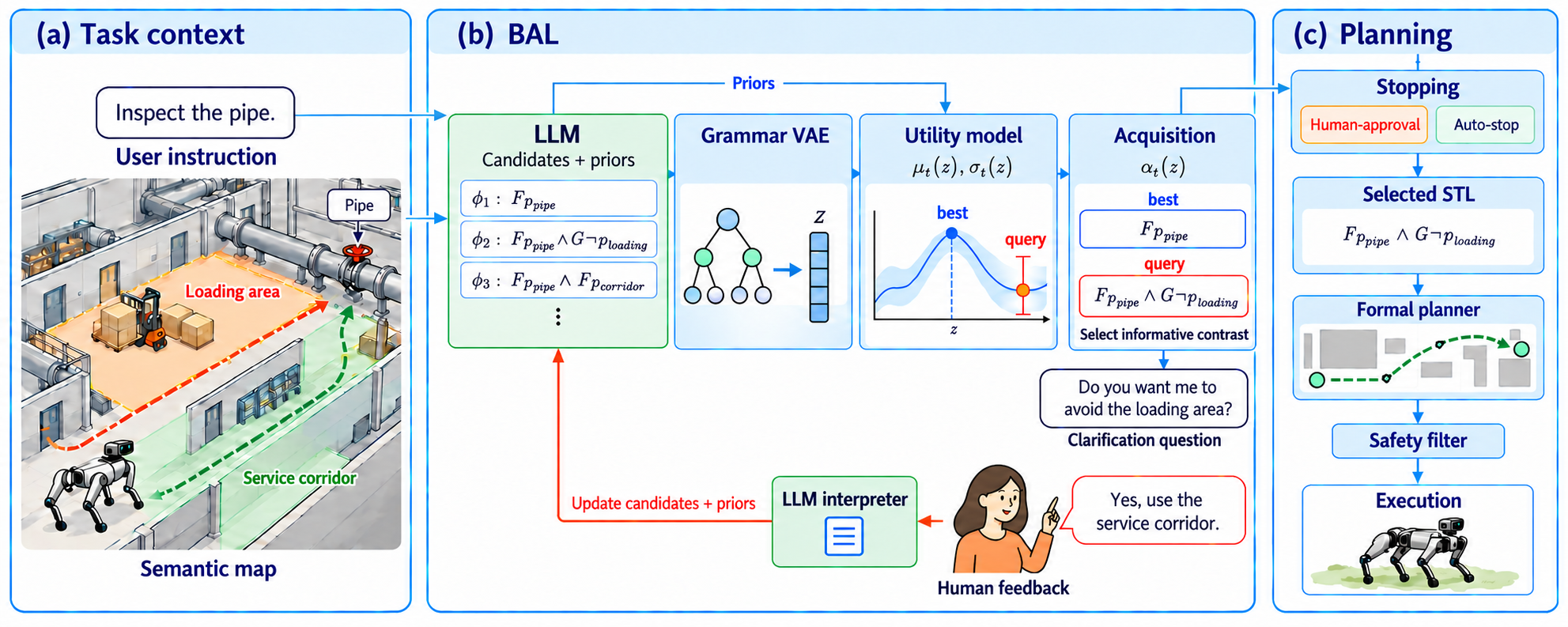
Ambiguous instructions leave object identity, ordering, timing or avoidance unstated. Translating the first utterance directly into a formal plan can therefore verify the wrong task. This work places a separate inference loop before planning: preserve multiple grounded hypotheses, choose informative distinctions and use answers to update their estimated utility. The hypothesis space must already express the intended task.
2 Related Work
The method combines language-to-formal-planning pipelines, interactive clarification and active preference learning.
2.1 Language-Conditioned Formal Planning
Prior systems translate language into planning languages or temporal constraints and then invoke a solver. BAL targets the preceding ambiguity problem: deciding which specification should be solved [LLM+P]. A valid solver output alone cannot certify that translation captured the user’s intention.
2.2 Multi-Turn Clarification
Free-form multi-turn dialogue can retain mistaken assumptions or stop too confidently. BAL gives the question generator a contrast selected by a probabilistic model, while still relying on language-model verbalization and answer interpretation. This external structure reduces some dialogue failures without making those semantic steps error-free.
2.3 Preference Learning in Human-Robot Interaction
Active preference learning often estimates reward features from comparisons or corrections. Here the learned alternatives are grounded logical specifications, which can be passed directly to a planner [active preference learning]. The change provides a clearer connection to task satisfaction while restricting intent to the chosen grammar and predicates.
3 Method
Inference and execution are separate: estimate the task specification from clarification, then synthesize a trajectory satisfying that estimate.
3.1 Problem Formulation
A grounded scene supplies objects, regions and admissible predicates. The unknown utility of a formula measures how closely it matches the user’s intended task; the goal is to select the highest-utility formula. Representability within the scene-specific specification space is an assumption, not something the dialogue can establish.
Equation 1
| (1) |
3.2 STL Specification Space
Signal Temporal Logic combines grounded predicates with Boolean operators and bounded eventually, always and until operators. A trajectory’s robustness gives a quantitative satisfaction test. These constraints express goals, avoidance and temporal relations, but their physical meaning depends on accurate grounding and the modeled trajectory.
3.3 Latent Utility Model over Specifications
A grammar VAE maps discrete formulas to continuous latent vectors, allowing a Gaussian process to model their utility [grammar VAE]. Initial observations are language-model-assigned candidate scores. The posterior therefore quantifies uncertainty under this surrogate and scoring model; it is not independently calibrated certainty about the human’s intent.
Equation 2
| (2) |
3.4 Active Clarification Query Selection
Pair the current candidate with highest posterior mean with a continuously optimized challenger. The acquisition combines information gain and a utility bonus, but reported experiments set the bonus to zero. Decode the challenger, ask a natural-language question about a distinguishing attribute, and score affected candidates from the answer. A cumulative deduplicated pool preserves previous hypotheses. Exploration can reach formulas never proposed by the language model, although interpretation and score updates still pass through that model.
Equation 3
| (3) |
3.5 Stopping, Specification Selection, and Planning
Plan for the current best specification at every round. Stop when the selected criterion succeeds or the query budget is exhausted, then return the current specification and trajectory. The generic algorithm permits user approval; the experimental implementation usually substitutes a verifier that knows the hidden ground-truth task.
Equation 4
| (4) |
4 Experiments
Two simulation domains test clarification systematically, while a separate web study and two Go2 deployments probe narrower human and physical settings.
4.1 Simulation Domains
Panda and City use different representations and planning backends, preserving the common specification-inference loop.
Franka Panda
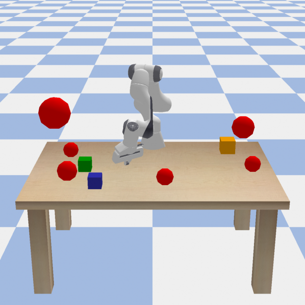
Panda has fourteen labeled tabletop objects with colors, geometry and positions. Reach/avoid predicates describe end-effector regions, and a gradient-based optimizer maximizes temporal-logic robustness. This is geometric reaching and avoidance, not a complete grasping or object-use benchmark.
City
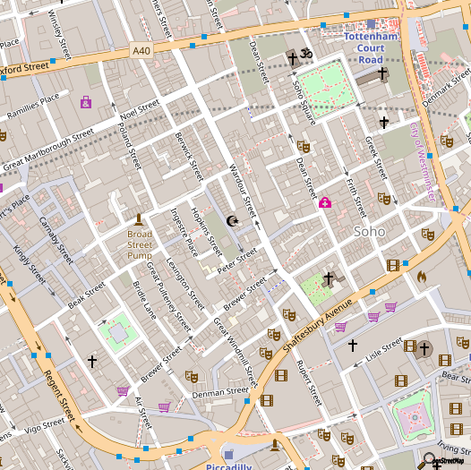
City uses forty landmarks and a semantic transition system without metric coordinates. Tasks use LTL, translated to an automaton and solved on a product system. This tests Boolean temporal/grounding ambiguity rather than seconds-level timing.
4.2 Test Scenarios
Tasks sample single-goal, multi-goal, sequential and partial-order templates, then discard cases for which the corresponding planner cannot find a satisfying trajectory. Ambiguity is injected into grounding, constraints and timing. A fixed proxy sees the hidden specification and answers only the requested aspect. This low-initiative protocol makes question selection important but narrows the range of natural human interaction.
4.3 Baselines
LM clarifies freely and emits executable waypoints or landmark sequences. LM+P uses free-form clarification but emits one formal specification for the same planner as BAL. That comparison helps separate the value of inference structure from simply adding a solver, although the prompts and model roles also differ.
4.4 Metrics
The main budget is ten questions. Success means the proposed trajectory satisfies the ground-truth specification, and the interaction stops at the first verified success. Runtime includes language calls, latent inference, acquisition optimization and planning. Rounds must be read with success and the budget, since early failure can otherwise look efficient.
4.5 Results
The results favor structured clarification across the tested model/domain combinations, with important ties and individual exceptions.
| Base Model | Panda | City | ||||
|---|---|---|---|---|---|---|
| BAL | LM | LM+P | BAL | LM | LM+P | |
| Success Rate (%) | ||||||
| GPT-5.4 | 91.14.2 | 48.97.5 | 82.25.7 | 62.59.9 | 29.29.3 | 20.88.3 |
| GPT-5.4-mini | 93.23.8 | 64.47.1 | 86.75.1 | 64.711.6 | 20.88.3 | 12.56.8 |
| Claude-Opus-4-6 | 91.14.2 | 64.47.1 | 82.25.7 | 50.010.2 | 29.29.3 | 20.88.3 |
| Claude-Sonnet-4-6 | 91.14.2 | 73.36.6 | 86.75.1 | 41.710.1 | 29.29.3 | 8.35.6 |
| Gemini-3.1-Pro | 91.14.2 | 82.25.7 | 91.14.2 | 54.210.2 | 33.39.6 | 25.08.8 |
| Gemini-3.1-Flash-Lite | 93.33.7 | 64.47.1 | 91.14.2 | 66.79.6 | 29.29.3 | 12.56.8 |
| Rounds of Clarification | ||||||
| GPT-5.4 | 2.330.41 | 6.160.62 | 3.510.54 | 6.540.57 | 9.140.31 | 9.170.30 |
| GPT-5.4-mini | 2.090.36 | 5.400.58 | 3.240.51 | 6.460.70 | 9.420.30 | 9.530.28 |
| Claude-Opus-4-6 | 2.930.47 | 4.690.62 | 3.380.52 | 7.250.53 | 8.750.39 | 8.940.41 |
| Claude-Sonnet-4-6 | 3.090.48 | 4.490.60 | 3.020.50 | 8.110.49 | 8.670.39 | 9.390.33 |
| Gemini-3.1-Pro | 2.360.42 | 3.470.49 | 3.160.45 | 7.780.56 | 8.830.39 | 9.060.34 |
| Gemini-3.1-Flash-Lite | 2.440.35 | 5.420.62 | 3.130.47 | 6.140.59 | 8.830.42 | 9.530.23 |
Task Performance
Across six backbones, BAL’s Panda success is 91.1–93.3% and City success is 41.7–66.7%, matching or exceeding the comparison methods. Planner-only augmentation helps Panda but can hurt City when the inferred formula is wrong. BAL usually asks fewer questions; one exception is Panda with Claude-Sonnet-4-6, where LM+P reports 3.02 rounds versus BAL’s 3.09. Table 1 retains all means and standard errors.
Cost Analysis
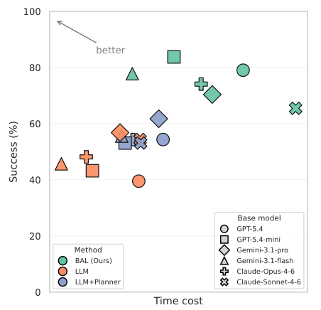
Latent inference and acquisition add computation, but fewer dialogue calls can offset it. Figure 3 compares complete wall-clock task time against performance, including smaller models that benefit from the structured pipeline. This is an empirical cost trade-off under the tested backends, not a universal latency or scaling law.
5 Ablation Study: Stopping Criteria
The Panda auto-stop ablation ends BAL when candidate-pool posterior differential entropy fails to decrease for two consecutive rounds. Language baselines decide when they have enough information. BAL retains similar success while the baselines stop earlier with lower success. Entropy stabilization is a heuristic stopping signal under the fitted model, not proof that the intended task has been identified.
6 User Study
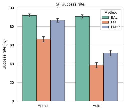
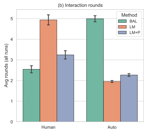
Thirty participants each complete six City episodes, two per method, with at most five rounds and simpler tasks. BAL achieves 0.65±0.07 success and 3.67±0.21 rounds, versus LM’s 0.48±0.07 and 4.38±0.14, and LM+P’s 0.37±0.06 and 4.25±0.15. Repeated-measures tests report overall method effects for success (p=.004) and rounds (p=.001). These omnibus results alone do not establish every pairwise contrast. Participants answer about assigned ground-truth tasks; automated verification determines success.
7 Real-World Deployment
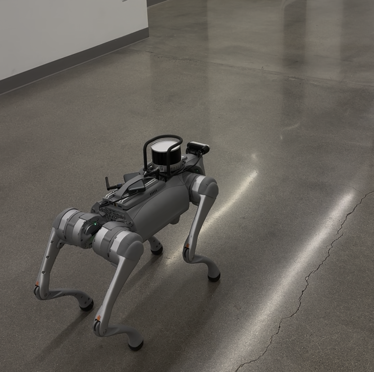
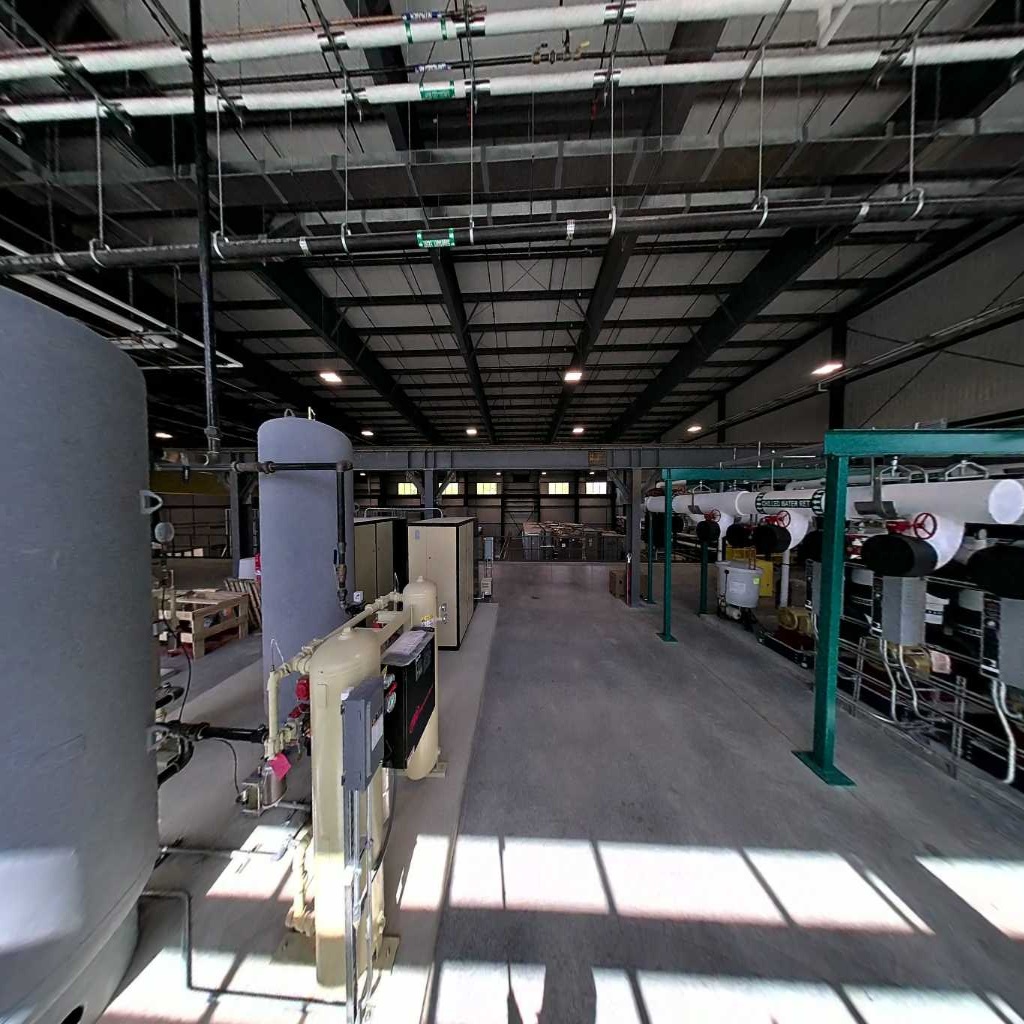
A Go2 executes plans in reconstructed School and Factory sites using semantic maps, a mixed-integer planner and local MPC/CBF control. Ten ambiguous instructions per site use Gemini-3.1-Flash-Lite and a ten-question cap. BAL succeeds on nine of ten at each site. It ties LM+P’s Factory success and School mean round count; other comparisons favor BAL. These selected feasible tasks use simpler temporal settings than the larger simulation sweeps.
8 Discussion
The approach improves clarification in the tested settings, but assumes a known task grammar and an accurate, relatively static world model. Missing predicates, changing scenes, language-model interpretation errors and correlated score errors can invalidate its inference. The human study uses one domain and constrained respondents; naturalness, broader preferences and uncertain grounding remain open.
ACKNOWLEDGMENT
The authors acknowledge support from the MIT × GE Vernova Energy and Climate Alliance for autonomous field inspection research.
Appendix
The appendix retains the inference algorithm, detailed protocols, control stack, human-study procedure and complete printed prompt templates.
Appendix A Pseudocode of Bayesian Active Learning Algorithm
Algorithm 1 alternates utility fitting, selection of the current best formula, planning, stopping checks and informative challenger queries. New answers update the candidate pool and noisy utility data. The returned plan satisfies the inferred task under the chosen planner, while ground-truth intent remains the inference target.
Appendix B Additional Results
Additional results separate physical task success from the clarification process that precedes execution.
B.1 Real-world Deployment Results
School success is 90/60/80% for BAL/LM/LM+P; Factory is 90/80/90%. Mean rounds are 3.50/6.30/3.50 and 2.90/4.30/4.10 respectively. The authors report zero collisions and successful execution of approved tasks. Twenty instructions across two mapped sites provide deployment evidence, not a universal collision guarantee.
Appendix C Implementation Details
Implementation details specify the grounding interface, utility-learning loop and domain-specific grammar VAE.
C.1 Context Inputs Across Domains
Each domain supplies logical predicates, a planning representation and a textual scene description. Their construction determines which task distinctions the system can discover.
School
School uses an offline dynamic scene graph from scans. Object boxes are padded to at least one square meter, objects outside rooms are removed, and room containment/semantic descriptions feed both prompts and mixed-integer constraints. These preprocessing choices simplify feasible footprints while changing the abstraction from raw geometry.
City (Lang2LTL OpenStreetMap).
City collects landmark names from the benchmark, normalizes them into predicate identifiers and infers coarse types by keyword matching. No coordinates are exposed; clarification focuses on name/type grounding in a topological system.
Factory.
Factory combines scanned geometry, vendor segmentation and expert corrections. Equipment records include function, material, inspection pose and relationships to neighboring/upstream/downstream equipment. This rich domain annotation is part of the deployment setup.
Franka Panda.
Panda records workspace limits, object positions/radii and goal/obstacle roles. Reach requires a downward-facing end effector inside a target sphere; avoid keeps it outside a buffered sphere. Feasibility-filtered formulas and their generated ambiguous instructions are fixed before method comparison.
C.2 Bayesian Active Learning Workflow
The active loop retains candidate histories while repeatedly refitting the utility surrogate and generating a new semantic contrast.
Candidate pool.
Maintain raw VAE latents and transformed GP inputs, plus a cumulative pool deduplicated by canonical formula strings. Each round asks for twenty fresh candidates conditioned on the original instruction, full dialogue and scene. Regeneration can revise the current pool without discarding all historical hypotheses.
Utility GP.
The utility surrogate uses a scaled Matérn-3/2 kernel with per-dimension lengthscales, normalized inputs and standardized outputs. Exact marginal-likelihood fitting estimates kernel and noise parameters; failed fitting retries with noise variance 0.01. Each observation is an integer score assigned by the language model, and the GP is refit from scratch. Expected improvement is diagnostic only.
Acquisition function.
The information-gain estimate uses 128 posterior draws and 128 likelihood samples per draw. Reported acquisition weights are 1 for information and 0 for posterior mean. Thus the challenger explores uncertainty while the separate best candidate supplies the exploitative anchor.
Equation
Best vs. challenger selection.
Choose the best pool element by posterior mean and optimize one challenger over bounded latent coordinates using five restarts and 256 raw samples. Decode and append that challenger. Grammar validity does not itself ensure physical feasibility or semantic relevance.
Prior bootstrap.
Bootstrap from the initial twenty language-model candidates and their utility estimates. This paragraph gives a 0–10 scale, while the printed candidate prompt uses 1–10; the source discrepancy is retained rather than silently resolved.
Question generation and answer parsing.
The verbalizer identifies a distinguishing attribute, asks one question and passes the answer back to a scoring/update call. Newly scored observations enter the utility dataset before refitting. Errors in this semantic interpretation can propagate through otherwise well-defined Bayesian updates.
C.3 Grammar VAE
A separate grammar-constrained variational autoencoder supports each domain’s formula vocabulary and timing discretization.
Grammar and AST encoding.
Parse formulas into preorder production-rule sequences and one-hot encode them, padding to length 100. The grammar includes Boolean/temporal operators, grounded propositions and clustered time bounds. Domain-specific terminals determine expressiveness.
Equation
Model architecture.
A two-layer bidirectional LSTM encodes formulas; a two-layer GRU decodes with a nonterminal stack and rule masks. Latent dimension is 16 and hidden width 256. Masking enforces syntactic admissibility, which is distinct from correct intent or satisfiable world constraints.
Training corpus.
Generate 100,000 formulas per domain with an 80/20 train/validation split. STL training bounds goals, obstacles and dependencies; LTL uses five to eight goals across selected templates with scaled obstacles. These distributions train the representation before clarification experiments.
Training objective and schedule.
Optimize reconstruction plus KL regularization for 150 epochs with Adam at 0.001, batch 32 and gradient clipping at 1. KL weight rises to one over ten epochs; free bits are disabled. Free-running decoding consumes previous soft predictions to reduce the training/inference mismatch.
Equation
Checkpoint selection.
Select the checkpoint with highest exact production-sequence reconstruction on validation, breaking ties by the variational objective. Each domain model trains on one RTX 5090. Exact reconstruction is a representation metric, not a task-success result.
Appendix D Evaluation and Deployment Setup Details
Evaluation uses fixed offline tasks; physical deployment deliberately uses a smaller, more constrained profile than the systematic simulation sweeps.
D.1 Setup Overview
A static manifest records each task’s parameters, hidden formula and ambiguous instruction. Methods share the same task/instruction pair, reducing variation from sampling or wording during comparison.
D.2 Shared Test-Case Generation
Generation combines template structure, grounded propositions and feasibility checks before introducing ambiguity.
Template families.
Single-goal and unordered multi-goal templates combine eventual reachability with avoidance. Sequential tasks impose a total order; partial-order tasks combine precedence and bounded-until constraints. Goal count alone does not capture structural difficulty.
Ground-truth sampling and feasibility filtering.
Sample goals/obstacles and timing within a 60-second horizon, then reject formulas that the domain planner cannot satisfy within its budget. This removes known infeasible ground truths but does not prove every later failure is exclusively a clarification error; planning or execution can still fail for an inferred task.
D.3 Systematic Ambiguity Injection
A deterministic plan removes roughly half of selected information along four axes: referential identity, temporal dependencies, goals/obstacles and time windows. Categories apply in order without double-counting omissions. Cache the plan and initial instruction for reuse. This controlled ambiguity distribution is narrower than unconstrained user language.
D.4 Simulation Evaluation Setup
The two systematic sweeps vary template structure, complexity, language backbone and random seeds with separate Panda and City planning backends.
Simulation complexity levels.
Panda varies one to five goals with one obstacle and one until clause. City varies five to eight goals with scaled obstacle/constraint counts. Complexity remains template-aware rather than reducing everything to the number of targets.
D.5 Real-World Deployment Setup
Physical tasks retain the same inference pipeline but simplify the specification space and insist on offline planner feasibility.
Deployment task profile.
Deployment rotates the relevant count through one, two and three, fixes one obstacle and uses roughly two to five grounded propositions. This is a selected simple-task regime, not the full simulation complexity grid.
Deployment feasibility check.
Check tasks with a 60-second planning horizon and nominal speed of 3 m/s. Resample up to ten times before dropping an infeasible cell. The nominal speed is a planning parameter, not a measured execution-speed claim.
Single-time-interval encoding.
A single time cluster maps every deployment interval to the full run, represented as [0,∞]. Tight metric deadlines appear only in multi-cluster simulation settings. Physical success therefore does not validate fine-grained deadline inference.
Robot execution.
Ground the selected formula, solve for waypoints and execute them on the mapped robot site. This tests integration of inference, mapping, planning and control under the deployment assumptions.
D.6 Human Proxy and Approval
The simulated respondent’s semantic role is separate from the ground-truth verifier that decides success.
Proxy conditioning.
The proxy sees the hidden task, scene and semantic primer, but must answer only the first question without exposing formulas or volunteering extra facts. Timing is expressed in ordinary seconds. This deliberately low-initiative respondent creates an information bottleneck.
Proxy/helper decoupling.
The detailed protocol fixes the proxy to GPT-5.4 with medium reasoning effort, independent of the helper model under test. Appendix H.2 contains a conflicting same-base-model statement; the edition records that inconsistency rather than treating both as equivalent.
Approval and termination.
A verifier checks each proposed trajectory against the hidden specification: sampled robustness for Panda and the appropriate mapped/discrete satisfaction test elsewhere. Success ends the run; exhausting ten rounds without satisfaction is failure. This implements the paper’s approval condition without requiring a person to inspect each trajectory.
Appendix E Safe Autonomous Navigation
The physical stack combines model-predictive tracking, a local barrier-function filter and the robot’s built-in locomotion controller. State estimation fuses odometry, inertial and LiDAR measurements.
Model Predictive Control with Safety Certificates
The optimization layers operate on simplified unicycle models and modeled obstacles; their certificates depend on those assumptions.
MPC planner.
MPC optimizes a receding-horizon second-order unicycle trajectory under dynamics, input and signed obstacle-margin constraints, executing only the first control before replanning. It supplies local goal-directed motion rather than verifying the entire natural-language task anew.
Equations 5
| (5) |
CBF safety filter.
A first-order-unicycle quadratic program minimally changes the proposed command while enforcing instantaneous barrier inequalities [CBF-QP]. Safety depends on the barrier model, state/obstacle estimates, feasible controls and tracking; this is not an unconditional physical guarantee under arbitrary uncertainty.
Equation 6
| (6) |
Low-level locomotion controller.
Convert the filtered result into forward velocity and yaw-rate commands for Go2’s built-in whole-body controller. Its tracking behavior links the simplified optimization models to the physical robot.
Appendix F Robotic Platform and Perception Stack
The deployment appendix documents hardware sensing and the planar mapping/localization abstraction.
F.1 Robotic Platform
Go2 supplies the mobile base, onboard interfaces and low-level locomotion control for the inspection/navigation demonstrations.
F.2 Sensor Suite
Supported sensing includes Unitree L1 or Hesai XT16 LiDAR, legged odometry, an IMU and RealSense RGB-D imagery. Geometry supports mapping and obstacle detection; visual semantics connect perceived objects to task predicates.
F.3 Mapping
Height-filter the 3-D point cloud, project it into a planar scan and build a 2-D occupancy grid. This makes standard navigation practical while discarding geometry outside the retained height band.
F.4 Localization
Adaptive Monte Carlo Localization combines planar scans and odometry in a particle filter on the occupancy map. Its estimated pose feeds MPC/CBF control, so localization quality affects both grounding and execution.
Appendix G Human User Study
The human study evaluates how well agents elicit information from constrained respondents about predefined City tasks.
G.1 Participants and Design
Thirty retained adult Prolific participants complete six episodes in about thirty minutes for US$6. Each sees two episodes per method; cyclic Latin-square ordering is counterbalanced and task order randomized. The study reports consent and exempt ethics review.
G.2 Task Setup and Participant Role
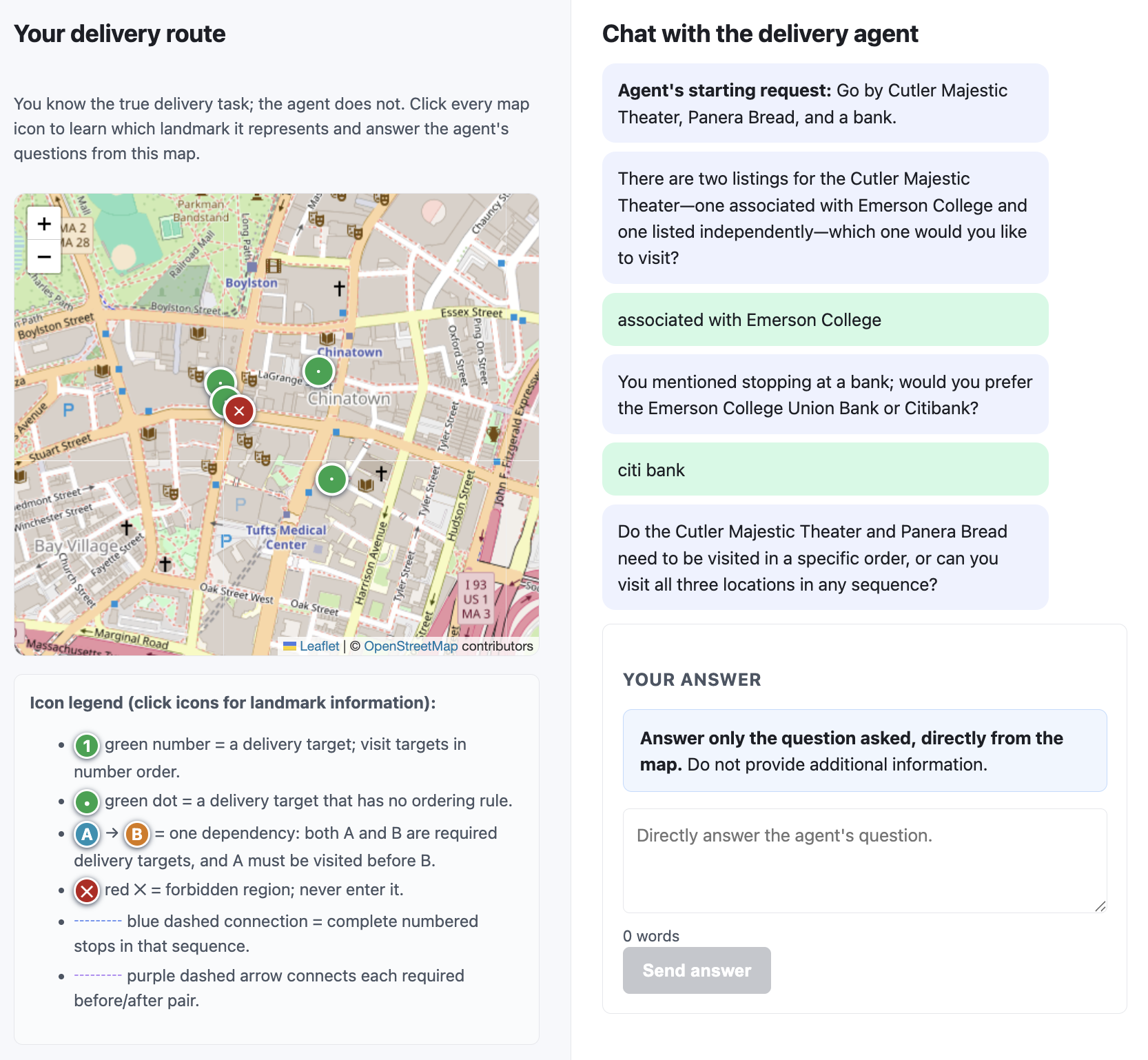
Participants receive an assigned map task and do not choose goals or write the initial instruction. Each case has four targets, one forbidden location and no until clauses, with multi-goal, sequential or partial-order structure. Respondents answer only what is asked, and each episode allows five clarification rounds.
G.3 Procedure and Interface
After a tutorial and comprehension check, participants answer in free-form language through the shared map/chat interface. Automated ground-truth verification ends successful episodes; participants are explicitly not asked to approve the generated plan. Figure 4 preserves the complete interface.
G.4 Outcome Analysis
Average each participant’s two episodes per method, then report means/standard errors over those thirty participant-level values. Repeated-measures ANOVA tests an overall method effect for success and rounds; the paper does not report every pairwise post-hoc result.
Appendix H Prompts
Seven printed prompt blocks are retained with their line breaks and placeholders. Some refer to example/rule blocks instead of printing their full contents; those omissions are properties of the source, not reconstructed material.
H.1 System design and role of LLMs
Each case combines a scene, hidden specification, ambiguous instruction, helper model and fixed proxy. Only the proxy-side generation/answering path and evaluation verifier are intended to know the hidden task.
LLM roles in BAL.
The helper proposes/scorers candidate formulas from the instruction and history, then verbalizes the selected contrast. Latent encoding, GP fitting, acquisition and formal planning are external computations. The implementation still relies on language calls for semantic candidate updates.
LLM roles in the baselines.
LM asks free questions and emits executable actions; LM+P asks the same style of questions but emits one formula for the shared solver. Their exact output schemas and context are preserved below.
LLM roles in the simulated user.
Proxy prompts generate the systematically ambiguous initial utterance and answer subsequent questions from the hidden task. The printed blocks constrain natural-language output and prohibit leaking formal notation.
H.2 Context parity across methods
Methods share scene context, admissible predicates where applicable, cached instructions and interaction budgets. The source’s claim here that proxy and helper share a base model conflicts with the fixed GPT-5.4 proxy specified in D.6 and H.1. Likewise, “proxy approval” is implemented by independent ground-truth verification in the detailed evaluation protocol.
H.3 Shared simulated-user prompts
The original instruction-generation and proxy-answer prompts remain below, including ambiguity categories, timing examples and the one-question response restriction.
P1 — Systematic ambiguous-instruction generator

Background: Signal Temporal Logic (STL) and templates

{stl_knowledge}


Ground truth intent for this scenario (for evaluation; do not reveal literally):

- Template: {template_name}

- Goals: {goals}

- Obstacles to avoid: {obstacles}

- Raw STL formula: {formula}


Task: Generate ONE short, natural-sounding navigation instruction for the ground-truth task above. Apply EXACTLY the ambiguity plan listed below — no more, no less. The target is ∼50% ambiguity per axis: about half of each axis is left unclear.


CATEGORY 1 — REFERENTIAL AMBIGUITY: {cat1_text}

CATEGORY 2 — TEMPORAL DEPENDENCY OMISSION: {cat2_text}

CATEGORY 3 — GOAL / OBSTACLE UNDERSPECIFICATION: {cat3_text}

CATEGORY 4 — TIME-INTERVAL OMISSION: {cat4_text}


ALL goals, obstacles, and constraints NOT listed above MUST appear: goals not in Cat. 1/3 by exact name; obstacles not in Cat. 3 stated as avoidance; dependencies/Until not in Cat. 2 stated explicitly; intervals not in Cat. 4 stated in precise seconds.


HARD RULES: 1. ONE short utterance (1--2 sentences). 2. No formal logic or option labels. 3. Preserve every Until clause unless explicitly in Cat. 2. 4. Output only the instruction text.
P2 — Proxy clarification answerer
Background — Signal Temporal Logic (STL) for robot navigation:
{stl_knowledge}
Your true intent is specified by the following ground-truth STL formula:
{gt_formula}
All STL interval values in the ground truth are REAL SECONDS in [0, 60]; 60 and inf mean the same thing. When the GT contains a TIGHT window, translate it directly into natural-language seconds:
F[10,30](enter(X)) → "reach X between 10 and 30 seconds in"
G[0,18](not_enter(Y)) → "keep clear of Y for the first 18 seconds"
G[12,48](not_enter(Y)) → "keep clear of Y between 12 and 48 seconds"
You are simulating a user answering a clarification question. Based ONLY on your true intent, answer the following in 1--2 short natural sentences, as a real user would. If the text contains multiple questions, answer ONLY the first. Do not mention formulas, option labels, or STL.
Clarification question: {question}
Your answer:H.4 BAL prompts
The candidate prompt requires consistency with prior answers and a scored formula array. The verbalizer uses contrasting formulas as inspiration for one open-ended question, with placeholders for ten examples. This is richer than a forced binary preference response, so the GP observation remains a language-model interpretation of the answer.
R1 — Candidate generation + prior with NL feedback

You are an expert in Signal Temporal Logic (STL) for robot dog navigation in a building. The robot has limited sensing range therefore must enter the target object to inspect it.


Generate {n} different valid STL interpretations of the instruction. For EACH interpretation, rate (1--10, 10 = perfect match) how well it captures the user’s intent.


Respond with a JSON array containing EXACTLY {n} elements, each with EXACTLY three fields:

- "stl_formula": full formula string

- "template_type": int 0|1|2|3

- "prior_score": int 1--10


[STL_FULL_FORMULA_EXAMPLES — canonical shapes for templates 0/1/2/3]

{context}


Original task instruction:

{instruction}


Clarification history so far (oldest → newest):

{qa_history}


Your job is to PROGRESSIVELY NARROW the space of plausible STL interpretations as more clarifications arrive:

- Every candidate MUST be consistent with every prior answer.

- Commit to details the human has confirmed (specific goal, ordering, avoidance).

- Focus remaining diversity on STILL-ambiguous dimensions.

- If history pins down the true intent, concentrate prior_score on the matching formula.

- If the human said "no" to avoidance/ordering/multi-goal, do NOT re-add those clauses.


[STL_FULL_FORMULA_EXAMPLES + INTENT_DIVERSITY blocks repeated]


Generate {n} different valid STL interpretations; same JSON schema as R1a.

Pay attention to timing cues from BOTH the original instruction and the clarification history. Copy concrete second numbers into ts/te and preserve them across regenerations.
R2 — Clarification-question verbalizer for BAL
You are helping a robot dog understand a human’s navigation instruction. You are shown the original instruction, the full clarification history, and two specific candidate STL interpretations (Option A and Option B). The two options are ONE example of a dimension that is currently ambiguous — use them as inspiration but write a HIGH-LEVEL OPEN-ENDED question that reveals NEW intent.
Guiding principles:
- Read the clarification history first. Do NOT re-ask resolved dimensions.
- Prefer OPEN-ENDED over forced binary choices.
- Consider every axis: which one, when (deadline), not before when (start), for how long (duration), in what sequence, all vs. any, anything to avoid.
- If options differ on a TIME-WINDOW dimension, ASK in concrete seconds.
- Never say "Option A"/"Option B"/"STL"/"formula". Do not quote 𝚎𝚗𝚝𝚎𝚛(⋅) predicates. 1 sentence.
[10 ICL exemplars covering goal/obstacle/order/duration/until]
{context}
Original instruction: "{instruction}"
Clarification history so far: {qa_history}
Option A: {stl_a}
Option B: {stl_b}
Respond with ONLY the question.H.5 LLM baseline prompts (clarification-only)
The free-form baseline can ask one short question or emit DONE, and its planning prompt outputs waypoints or INFEASIBLE. These complete printed templates are preserved, including formatting and horizon/speed constraints.
R2 — Free-form clarification asker

Context (environment and areas):

{context}

User instruction: {instruction}

So far you have asked the following clarification questions and received answers: {qa_block}


You are deciding between two actions this round:

 (a) Ask exactly ONE more short clarification question, OR

 (b) Stop because you already have enough information.


Useful topics: which goal area, area arrival deadline, goal start window (earliest start), how long to avoid an area, visit order between goals, areas to avoid. Prefer concrete second numbers over vague "soon/later".


Output rules (pick exactly one format):

 (a) one short question ending in "?". No compound questions, no "and"/"also"/"then", no bullets, no preamble.

 (b) the single literal token DONE on its own line, no other text.
Rplan — clarification → waypoints
You are a robot navigation planner. The user gave an ambiguous instruction; you asked clarification questions and received answers. Now output a single trajectory as a JSON array of waypoints.
Environment and areas (with bounding boxes):
{context}
Original instruction: {instruction}
Clarification Q&A:
{qa_block}
Requirements:
- The first waypoint must be exactly the robot’s start position in the context.
- Waypoints must lie strictly within the room boundaries described above.
- Each waypoint is {"x": float, "y": float, "t": optional float}.
If the requested constraints cannot all be satisfied within the horizon and the robot’s speed limit, output the single token INFEASIBLE on its own line. Otherwise output only the JSON array, no other text.H.6 LLM+P baseline prompts (clarification → formal spec → planner)
The planner-augmented baseline requests exactly one candidate formula using the same schema and shared formal-planning backend. Its printed template refers back to common rule/example blocks; those references remain intact.
Rspec — single best STL/LTL formula
under full Q/A history

[Same body as BAL R1 — {context}, {instruction}, {qa_history}, the same FULL_FORMULA_EXAMPLES, INTENT_DIVERSITY, TIMING_HARD_RULES, NESTING_RULES blocks]


Generate 1 valid STL interpretation. Respond with a JSON array of EXACTLY one element with the standard schema (stl_formula, template_type, prior_score). The downstream planner will lift this formula into a trajectory using the same MILP / gradient / Spot pipeline BAL uses; do not emit waypoints.