Overview
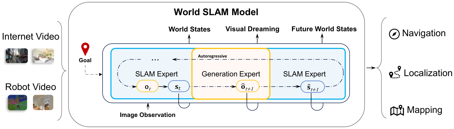
World SLAM Model combines visual prediction, geometric state estimation, persistent history, and local refinement for goal-directed navigation.
At a glance
WSM generates future RGB observations conditioned on a metric goal, then estimates their camera poses and depth to form a navigation plan. The same geometric experts update state from actual observations, with cached history and within-chunk refinement. Simulated navigation improves over the tested baselines, while aligned pose accuracy improves but dense reconstruction remains weaker than fine-tuned SLAM-Former. The system needs RGB observations plus a goal position; it does not use measured depth or external odometry during navigation.
1 Introduction
The paper argues that navigation can benefit from how SLAM maintains and revises spatial state, not only from an externally supplied map. WSM jointly trains visual generation and geometric estimation, then repeatedly predicts, executes, observes, and updates. Its persistent state anchors generated plans to a goal in the first-camera frame. Evaluation is in simulation; the paper does not demonstrate a physical-robot deployment.
2 Related Work
The work connects learned SLAM and reconstruction, visual navigation, and predictive world models.
2.1 SLAM and Feed-Forward 3D Reconstruction
Classical SLAM optimizes trajectories and geometry over time, while learned models regress them directly or maintain streaming state. SLAM-Former (Yuan et al., 2026b) is the main geometric comparator. WSM adds navigation-conditioned prediction to a shared state-estimation architecture; its implemented backend refines recent frames within a chunk rather than providing unrestricted global loop closure.
2.2 Visual Navigation
End-to-end planners often rely on externally supplied pose or depth. LoGoPlanner (Peng et al., 2025) grounds planning in pretrained geometric features and serves as a strong benchmark comparison. WSM estimates geometry internally from RGB, while still receiving a metric goal and using a low-level trajectory-tracking controller.
2.3 World Models
Video world models can predict future views or action-conditioned evolution. WSM couples this prediction to an incrementally maintained spatial state so generated views can be converted into camera motion and compared with actual subsequent observations.
3 World SLAM Model
The model integrates visual dreaming, metric-state estimation, and action execution through a common autoregressive history.
3.1 Overview
A causal video autoencoder compresses four raw frames into each latent frame. State at a latent step contains depth and four corresponding camera poses. Processing occurs in chunks of latent frames, with all poses represented relative to the initial camera.
Method overview.
The method first defines prediction and geometric recovery, then their shared architecture, joint training, reinforcement post-training, and closed-loop inference.
3.2 Video Model and SLAM Model for Navigation
The formulation distinguishes predicted visual appearance from metric motion. A generated video becomes a usable navigation plan only after geometric estimation recovers its camera trajectory.
Dream for visual states.
The generation expert predicts future RGB conditioned on observed images and estimated history states. Its output is a possible visual continuation rather than a directly issued robot action.
Equation 1
| (1) |
SLAM for world states.
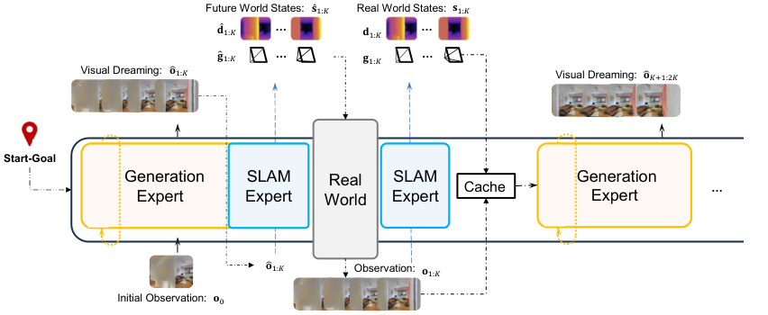
The same SLAM expert estimates poses and geometry for both observed and imagined sequences. Applied to a predicted transition, it acts as an inverse model that recovers camera motion. A local backend jointly re-estimates recent states within the active chunk and updates their cached representations.
Equations 2–4
| (2) |
| (3) |
| (4) |
Start-goal navigation.
A three-dimensional goal position in the initial-camera frame conditions generation; no goal orientation is specified. Recovering poses from the goal-conditioned video yields the proposed metric trajectory.
Equation 5
| (5) |
3.3 Unified Architecture and Autoregressive Modeling
Three transformer experts exchange information through joint attention, with separate prediction and context tokens controlling what each task can observe.
Architecture.
The RGB generation expert and separate depth and pose experts form one mixture-of-transformers model initialized from Wan (Wan et al., 2025). RGB and depth use the video autoencoder; a pose head decodes camera motion. Goal cross-attention enters the generation expert only. Shared attention links modalities, while expert parameters remain distinct.
Training sequence.
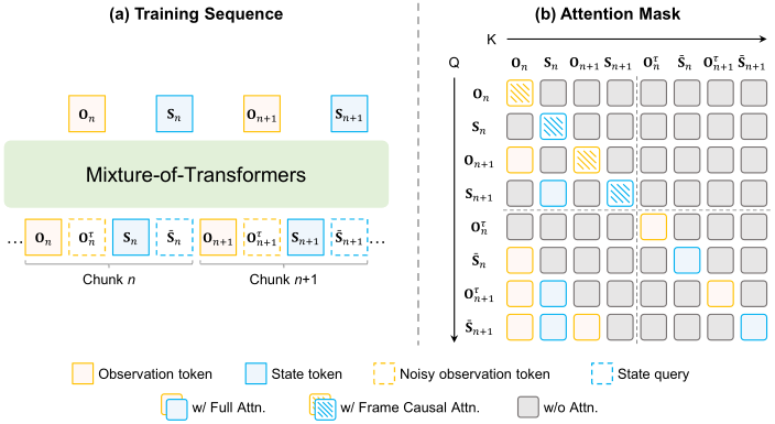
Teacher-forced training includes clean context tokens plus noisy RGB prediction tokens and fixed depth/pose queries. Multiple chunks are supervised in parallel, allowing generation and state estimation losses in one forward pass.
Attention mask.
The attention mask preserves chunk order and prevents prediction tokens from reading their own targets. Clean RGB and state histories remain separate. RGB prediction sees earlier clean context and its own chunk’s noisy tokens; state queries additionally see current clean RGB. Prediction streams do not directly read each other’s targets.
3.4 Training
Training first learns joint visual and geometric prediction, then adapts which futures are generated using map-based rewards.
Pretraining: joint teacher-forcing training.
Flow matching trains RGB generation, while regression supervises depth latents and absolute/relative camera poses. The losses share the model and coordinate frame. This joint objective provides geometric supervision during pretraining; it is not learned purely from unlabelled navigation videos.
Equations 6–7
| (6) |
| (7) |
Post-training: safety-prioritized reinforcement learning.
DiffusionNFT (Zheng et al., 2026) post-trains only self-attention adapters in the generation expert. Sixteen dreamed trajectories per query are recovered by the frozen SLAM expert and scored against dataset occupancy maps and expert geodesic progress. A collision gate prioritizes free-space trajectories, while progress matching allows routes that differ spatially from the demonstration. Freezing the estimator prevents direct reward improvement by modifying that estimator, but does not guarantee correct geometry or collision prediction under all generated inputs.
Equation 8
| (8) |
3.5 Autoregressive Closed-Loop Inference
At each step, WSM generates future views, estimates their states, and executes a short pose prefix. New real observations replace the imagined continuation in persistent history. The backend revises depth and poses within the current chunk while leaving RGB tokens fixed; completed chunks are no longer refined. Dreamed frames are discarded after planning. This maintains observation-grounded history with bounded local revision rather than accumulating unverified imagined states.
4 Experimental Evaluation
Evaluation separates navigation success, geometric accuracy on held-out trajectories, and ablations of joint SLAM prediction, local refinement, and post-training.
4.1 Experimental Setup
Training and inference use different hardware and evaluation domains; the original tables preserve their complete settings.
Training data and details.
InternVLN-N1 provides training data, with 5% of trajectories held out from both training stages for geometric evaluation. Ten pretraining epochs and one post-training epoch use 48 A100 GPUs. Generation, depth, and pose widths are 3,072, 1,536, and 768, initialized by adapting pretrained video-model weights. A held-out trajectory split should not be equated with a held-out scene split.
Inference details.
Inference on one RTX 4090 generates four future latents at 320×192 using eight sampling steps, yielding sixteen poses. The controller executes through the fourth pose before replanning from four new observations. History retains up to 128 observed latent frames. The paper does not report full planning latency or hardware control frequency.
4.2 Navigation Evaluation
The navigation benchmark has forty training-disjoint environments—twenty Home and twenty Commercial—with one hundred episodes each. The goal remains fixed in the initial-camera frame. Success requires slowing or stopping within one meter of it, so this is not a precision docking criterion.
WSM reaches 70.3% Home success and 73.9% Commercial success, with SPL 66.3% and 71.8%. Against the authors’ LoGoPlanner re-evaluation, success gains are 10.7 and 8.1 percentage points. Both published and re-evaluated baseline numbers remain in Table 1. The result is strongest among the evaluated methods under this simulation protocol, not a broad claim over every navigation system.
| Method | Input | Home | Commercial | |||
| RGB | Depth | SR | SPL | SR | SPL | |
| DD-PPO (Wijmans et al., 2019) | 0.4 | 0.4 | 5.3 | 5.2 | ||
| iPlanner (Yang et al., 2023) | – | 43.0 | 40.6 | 54.6 | 52.8 | |
| ViPlanner (Roth et al., 2024) | 45.0 | 43.2 | 63.7 | 61.9 | ||
| LoGoPlanner (Peng et al., 2025) | 57.3 | 52.4 | 67.1 | 63.9 | ||
| LoGoPlanner† (Peng et al., 2025) | 59.6 | 53.6 | 65.8 | 62.0 | ||
| World SLAM Model | – | 70.3 | 66.3 | 73.9 | 71.8 | |
4.3 SLAM Evaluation
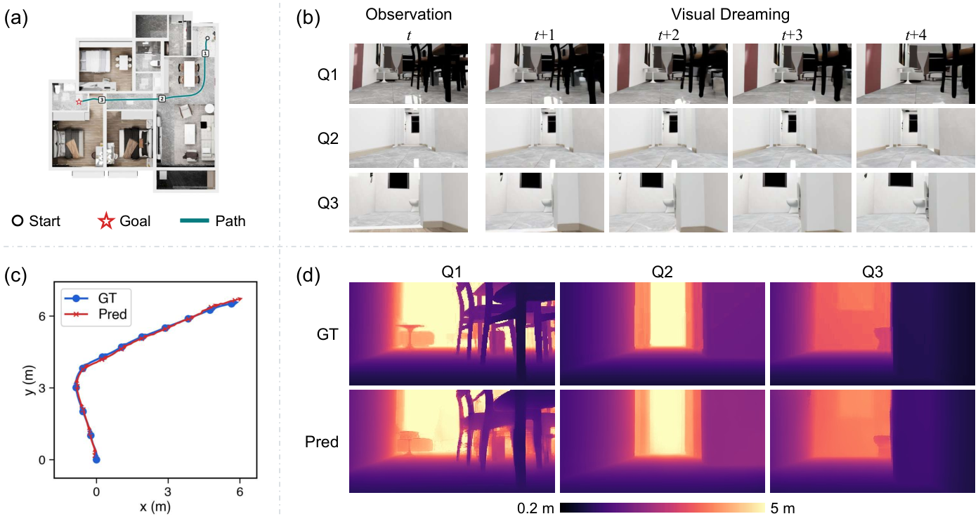
WSM’s camera-center ATE is 0.021 m versus 0.041 m for fine-tuned SLAM-Former, but dense reconstruction error is worse: 0.062 m versus 0.041 m. Pose evaluation uses per-sequence similarity alignment, and geometry additionally uses rigid ICP; these aligned errors do not alone establish absolute metric-scale accuracy. Input resolutions and initialization differ between models. Appearance-oriented depth latents are a proposed explanation for WSM’s weaker dense geometry, not an isolated causal finding.
| Method | ATE RMSE (m) | Acc. RMSE (m) |
|---|---|---|
| SLAM-Former† (Yuan et al., 2026b) | 0.051 | 0.057 |
| SLAM-Former‡ (Yuan et al., 2026b) | 0.041 | 0.041 |
| World SLAM Model | 0.021 | 0.062 |
4.4 Ablation Studies
Ablations test whether observed-state estimation and local revision contribute beyond decoding actions from imagined views.
SLAM IDM.
Removing the depth expert and observed-frame state estimation lowers pretrained-model success from 64.6% to 28.1% on Home and from 68.5% to 32.1% on Commercial. The comparison supports explicit state estimation in this setup, but removes several geometric components together and does not isolate depth, localization, and shared-state representation independently.
Local backend.
With matched post-training procedures, local refinement improves success by 2.0 points on Home and 1.3 on Commercial, and SPL by 1.1 and 1.3 points. The contribution is incremental beyond the shared pretrained model and is limited to revision within the current chunk.
| Method | Home | Commercial | ||
|---|---|---|---|---|
| SR | SPL | SR | SPL | |
| IDM (w/o SLAM) | 28.1 | 27.1 | 32.1 | 31.2 |
| World SLAM Model (w/o post-training) | 64.6 | 61.5 | 68.5 | 66.9 |
| Method | Home | Commercial | ||
|---|---|---|---|---|
| SR | SPL | SR | SPL | |
| w/o local backend | 68.3 | 65.2 | 72.6 | 70.5 |
| w/ local backend | 70.3 | 66.3 | 73.9 | 71.8 |
5 Conclusion
Joint prediction and state maintenance improve simulated goal navigation while retaining useful geometric estimates. Depth encoded through an appearance VAE sacrifices some reconstruction fidelity. The uncompressed history cache grows in cost and is capped during inference, limiting long-horizon scalability. Geometry-specific latents, efficient history compression, and physical deployment remain open directions.
AI use statement
The authors disclose using generative AI for grammar correction and writing polish, state that they reviewed the assisted text, and take responsibility for the final content.
Appendix A Method Details
The appendix specifies depth and pose supervision and the map-scored reinforcement objective used for post-training.
A.1 Pretraining Objective
Pretraining combines flow-matching RGB generation with standardized depth-latent regression and absolute/relative pose losses.
RGB generation.
Flow time is sampled per chunk through a shifted distribution, and the loss uses a bell-shaped time weight. The first chunk is a clean visual anchor and contributes no generation loss.
Depth.
Depth is clipped to 0.2–5 meters, normalized logarithmically, replicated into three channels, and encoded by the video VAE. The model regresses standardized depth latents and reverses this mapping after decoding. The clipping range limits the explicit depth values represented by this pathway.
Equation 9
| (9) |
Camera pose.
Smooth-L1 losses supervise translation and unit-quaternion rotation for absolute poses and pairwise relative pose differences. Training uses metric first-camera-frame poses without scale alignment. This differs from the similarity-aligned pose metric used at evaluation.
Equation 10
| (10) |
A.2 Post-Training
Post-training uses dataset maps and trajectories as a reward source without running an interactive physics simulator.
Reward.
Recovered trajectories are placed in the occupancy map using the dataset pose of the query frame. Reward compares each step’s geodesic progress with the expert and checks the robot footprint against free space; the best safe candidate receives a margin-dependent bonus. Thus “simulator-free” post-training still requires map and pose supervision, and safety is judged in that map with estimated trajectories.
Equation 11
| (11) |
Objective.
Within each candidate group, standardized rewards become bounded optimality probabilities. DiffusionNFT combines positive and negative flow objectives with a reference-model regularizer, using an exponential-moving-average sampling policy. The retained algorithm shows the full procedure. It requires generated samples but not likelihoods or every intermediate sampling state.
Equations 12–13
| (12) |
| (13) |
Appendix B Experimental Details
Implementation details cover expert widths, optimizer schedules, adapter configuration, and additional qualitative and quantitative results.
B.1 Implementation Details
The following subsections and Tables 5–6 specify architecture and training settings needed for reproduction.
Architecture.
All experts have thirty transformer layers with joint attention. Generation retains the video backbone’s 3,072-wide hidden state and twenty-four heads; depth and pose use narrower interpolated weights. RGB and depth latents use 1×2×2 patches.
Pretraining.
Depth and pose loss weights are 1 and 0.5. Generation and goal embeddings use 0.3 times the base learning rate. Table 5 includes precision, batch size, schedules, clipping, and the ten-epoch training budget.
Post-training.
Post-training selects roughly 10% of trajectories as hard examples and trains rank-32 adapters with scaling 64 on generation self-attention projections. Each query uses sixteen four-latent dreams, eight sampling steps, and four sampled flow times per dream. Reward temperature is 0.01 m² and its goal radius is 0.2 m, distinct from the one-meter navigation evaluation threshold.
| Hyperparameter | Value |
|---|---|
| Initialization | Wan2.2-5B |
| Input resolution | |
| Chunk size (latent frames) | uniform in |
| Timestep shift | 5 |
| / / | 1 / 0.5 / 0.1 |
| Optimizer | AdamW (, , ) |
| Weight decay | 0.01 |
| Peak / final learning rate | / |
| LR multiplier (generation expert, goal embedding) | 0.3 |
| Schedule | 5% linear warmup, cosine decay |
| Gradient clipping | 2.0 |
| Epochs | 10 |
| Global batch size | 48 |
| Precision | bfloat16 |
| Hardware | 48 A100 GPUs |
| Hyperparameter | Value |
|---|---|
| Initialization | pretrained model |
| Trainable parameters | self-attention LoRA of the generation expert |
| LoRA rank / | 32 / 64 |
| Group size | 16 |
| Dreamed latent frames | 4 |
| Sampling steps | 8 |
| Flow times per dream | 4 |
| Timestep shift | 5 |
| Temperature / goal radius | 0.01 m2 / 0.2 m |
| / / | 0.1 / 5 / |
| Optimizer | AdamW (, , ) |
| Weight decay | |
| Peak / final learning rate | / |
| Schedule | 3% linear warmup, cosine decay |
| Gradient clipping | 1.0 |
| Epochs | 1 |
| Precision | bfloat16 |
| Hardware | 48 A100 GPUs |
B.2 Two-Stage Ablation
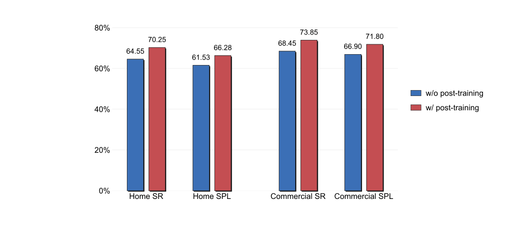
Post-training raises success by 5.7 points on Home and 5.4 on Commercial, with corresponding SPL gains of 4.8 and 4.9. Since the geometric experts are frozen, the change mainly concerns the generated future distribution, subject to the fixed estimator’s accuracy.
B.3 Additional Qualitative Results
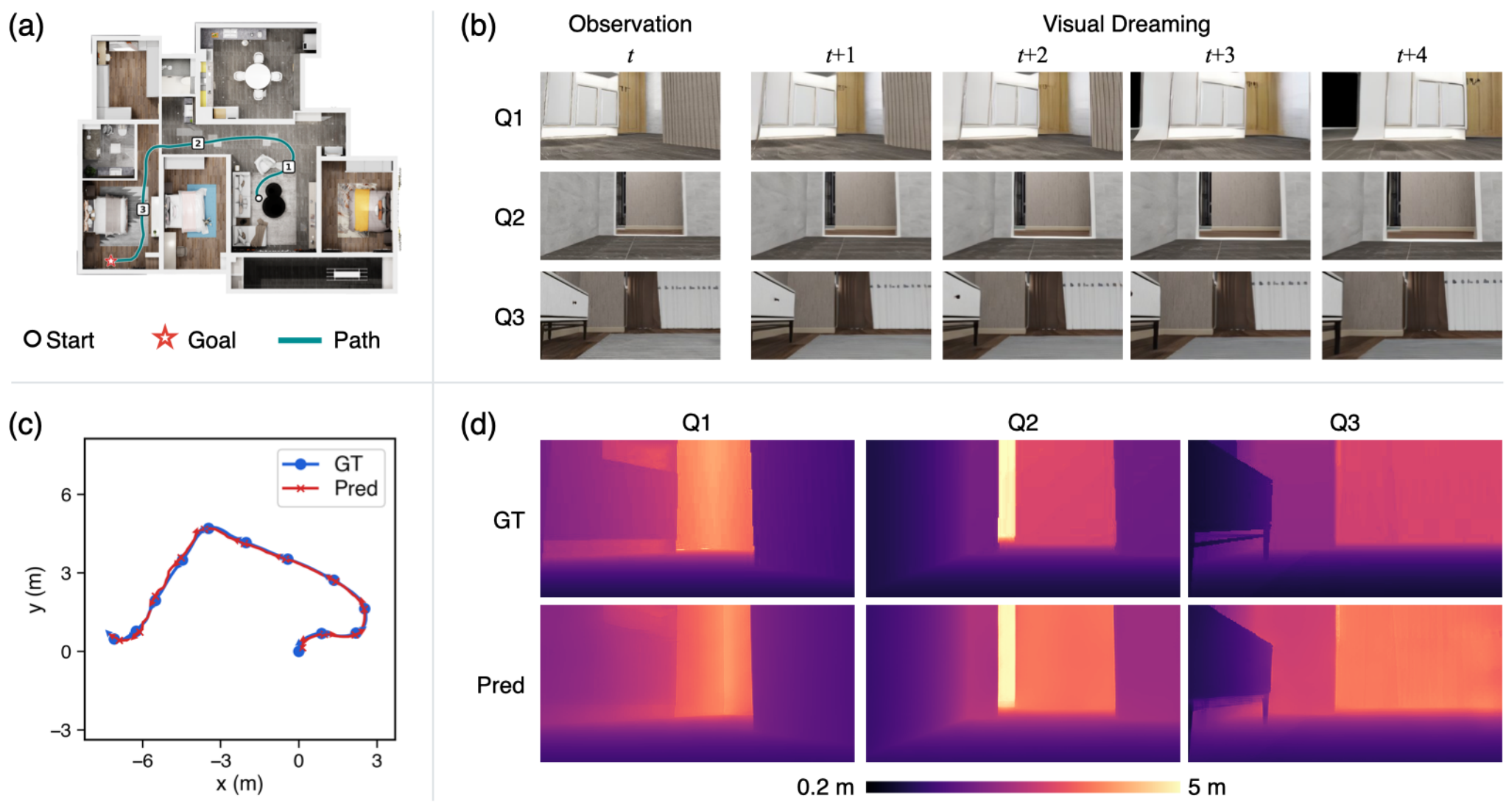
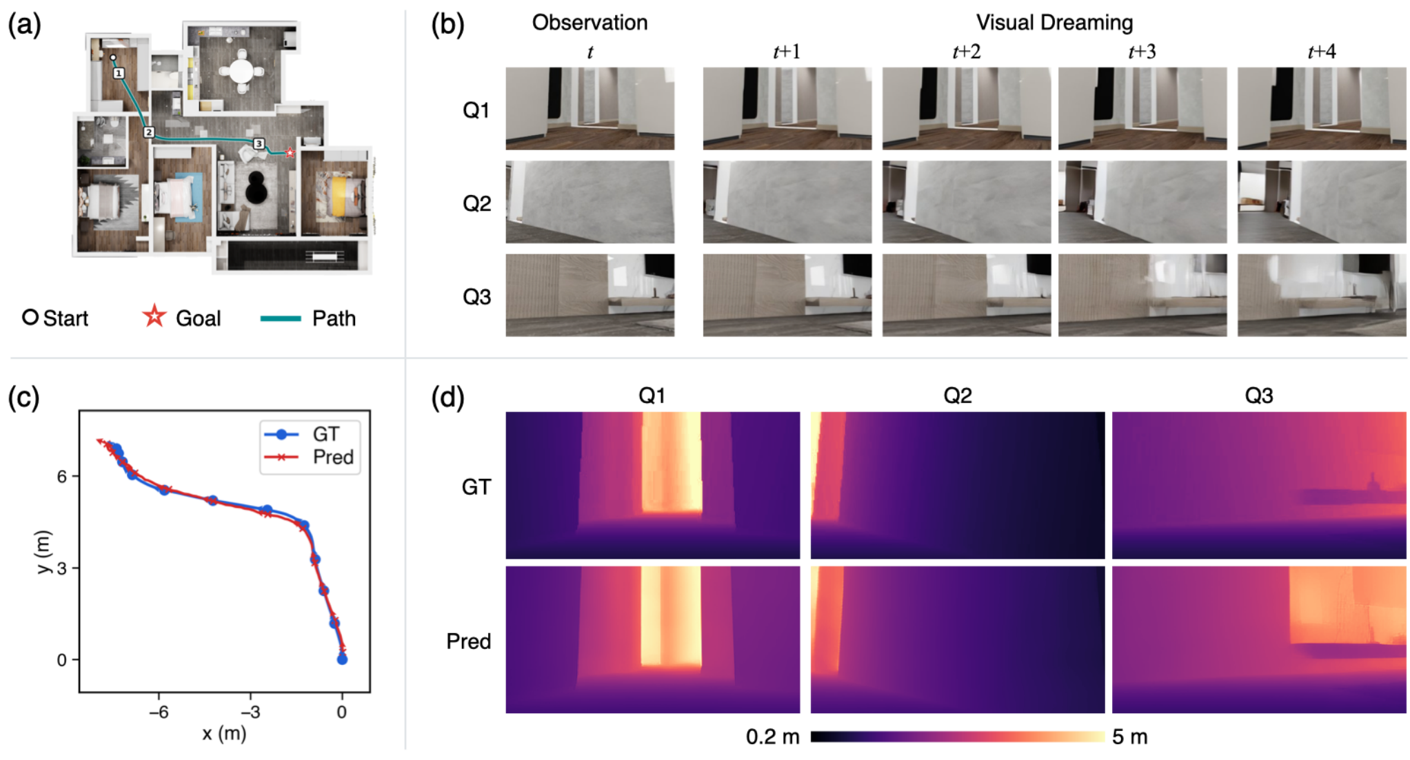
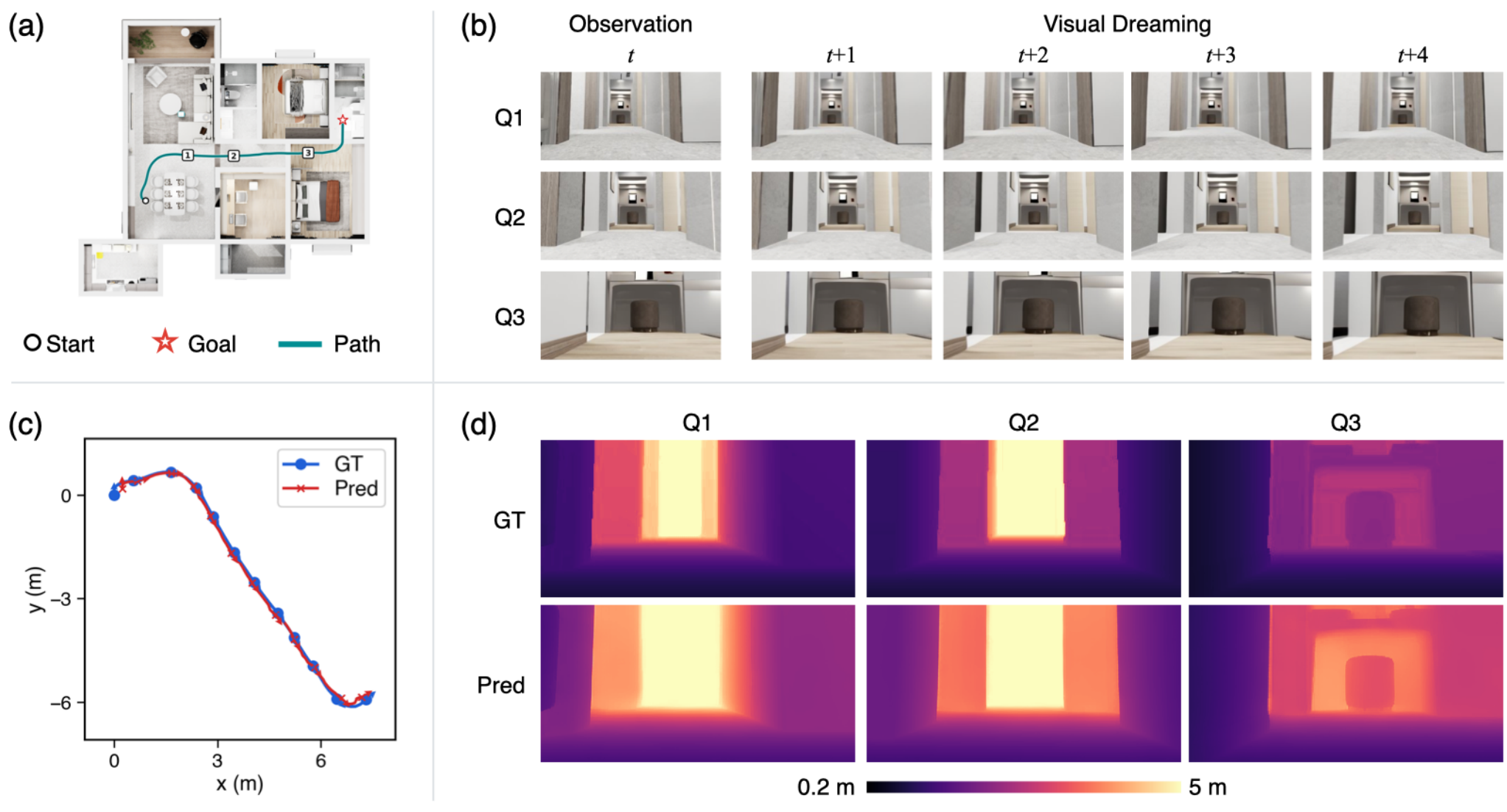
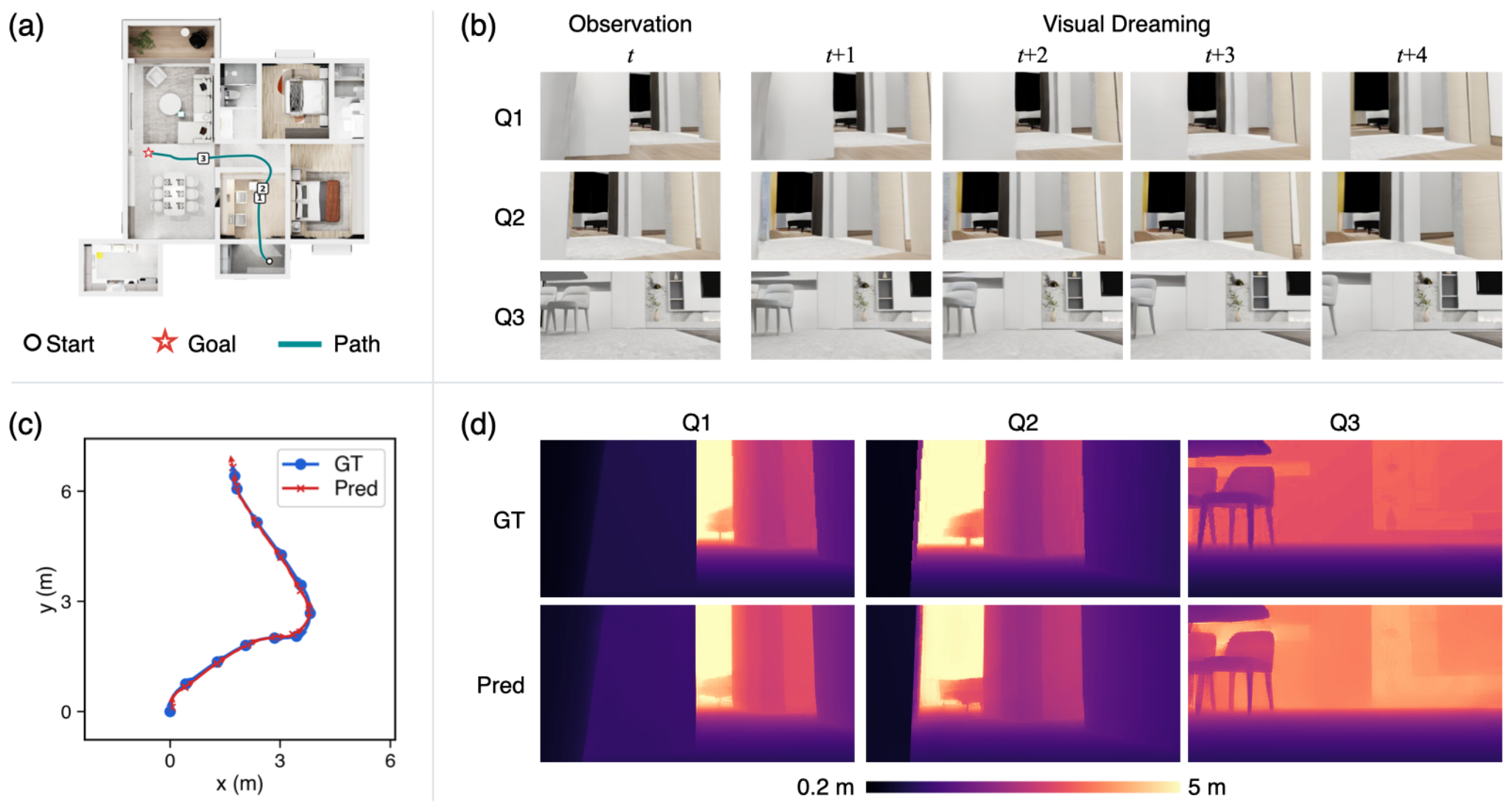
Figures 6–9 retain four additional simulated episodes from two Home environments, showing observations, generated views, estimated trajectories, and depth. These are qualitative examples rather than additional aggregate evaluation.