At a glance
Representation World Model (RWM) learns a latent space in which interpolating between the current and goal observations supplies a path that an inverse-dynamics model decodes into actions. Action supervision on constructed paths shapes the encoder; inference needs neither recursive forward prediction nor action-sequence search.
On four continuous-control benchmarks, the reported mean success is 98.25%, versus 96.86% for the strongest matched INTACT variant and 95.33% for its direct inverse-dynamics baseline. A separate LIBERO-Goal implementation reaches 93.0%, but substitutes a learned, task-conditioned latent-displacement predictor because goal images are unavailable. That result therefore tests an extended architecture.
1. Introduction
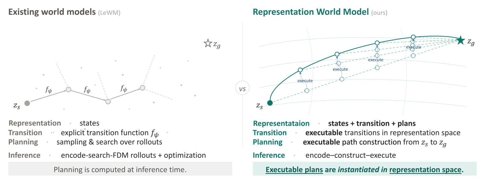
Predictive world models can learn useful state representations while leaving inference-time planning to sampled rollouts. RWM instead constrains the planning operation to straight-line construction in latent space and asks action supervision to organize the representation around that operation. Figure 1 contrasts these pipelines.
The intended division of labor is a structured encoder plus a shallow inverse-dynamics decoder. Avoiding online search does not eliminate learned computation: training must make endpoint-constructed transitions useful, and an action decoder still determines the controls. Interpolation by itself is not a feasibility guarantee.
2.1 Representation learning
Image and video representation methods organize features through invariance, prediction, or temporal structure [2] [3] [25]. RWM trains from action-labeled trajectories and applies supervision to the latent regions between observations, rather than only to the encoded observations themselves.
2.2 World models
World Models, PlaNet, Dreamer, and MuZero establish different ways to learn states and dynamics for decision making [12] [13] [16] [28]. LeWM predicts action-conditioned latent futures and uses representation regularization [21]. RWM removes the explicit forward predictor from its standard formulation, grounding representations directly through action recovery.
2.3 Planning with learned world models
CEM and MPPI search over candidate futures using learned dynamics. Direct goal-conditioned policies or inverse-dynamics models amortize control into a predictor [24]. RWM inserts an explicit geometric path between endpoint encoding and local action decoding. The distinction describes its architecture; the experiments do not prove that it solves every planning problem more generally.
3. Method
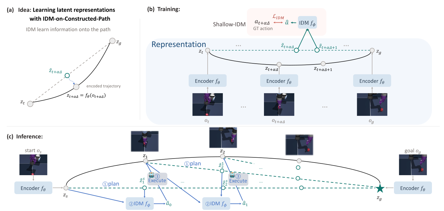
Figure 2 preserves the training and closed-loop inference diagrams. Only the encoder and inverse-dynamics model are learned in the standard goal-observed formulation.
3.1 Problem setup
Training uses offline trajectories of observations and associated actions. An observation or action may itself be a fixed-length chunk. Equation 1 maps observations to latent states. The following source equation states the conventional alternative: optimize an action sequence by recursively predicting a future state and comparing it with the goal.
Equations


3.2 Representation world model
Given two observations from the same demonstrated trajectory, RWM linearly interpolates their encoded endpoints. The interpolation coefficient is the intermediate time’s fraction of the endpoint interval. This construction defines a geometric location; executable behavior must be learned from the demonstrated actions.
Supervising intermediate points also updates the endpoint representations because all constructed points depend on them. This is the mechanism by which action loss can reshape the latent geometry.
Equation

Planning as a geometric operation
At inference, the same construction generates intermediate representations between the encoded current observation and encoded goal. Their ordered sequence is the latent plan. Every point is obtained directly from the endpoints rather than recursively from the previous predicted state.
The construction assumes a chosen temporal horizon. The paper does not supply a general mechanism guaranteeing a feasible straight latent path for arbitrary endpoints, obstacles, or multiple incompatible demonstrated routes.
Equation

3.3 Action-grounded representation learning
For a sampled trajectory segment, the model constructs neighboring points along the endpoint-interpolated path and compares their decoded actions with the segment’s recorded actions.
Action supervision on constructed paths
Equation 2 is mean squared action error along the constructed path. The shared inverse-dynamics model receives each adjacent pair of interpolated representations. Gradients pass through the interpolation to the encoder, encouraging both endpoint information and path geometry useful for action recovery.
Equation

Optional encoded-state supervision
An optional auxiliary loss applies the same inverse-dynamics decoder to consecutive encoded observations. Its complete formula is retained below. This term grounds actually observed transitions directly, while the main interpolation loss trains transitions through constructed states.
Equation
Why inverse dynamics shapes the representation
If all observations collapse to one code, the decoder receives identical inputs for distinct action targets and cannot fit them all. Likewise, merging configurations that require different actions creates conflicting supervision on their constructed paths.
This gives an optimization argument against trivial collapse for action-varying data, rather than a theorem guaranteeing unique state recovery or feasible plans. The probing and control experiments test what the learned representation retains in the studied environments.
Soft interpolation consistency
The optional consistency loss aligns constructed intermediate states with the encoder outputs at the corresponding demonstration times. It regularizes geometric alignment; it does not independently specify which task-relevant information the representation must preserve.
Equation
Overall objective
Equation 3 combines interpolation inverse dynamics, optional encoded-state inverse dynamics, and optional consistency with separate weights. The first term supplies the principal action-grounding signal. No explicit forward-dynamics model is trained for the standard formulation.
Equation

3.4 Rollout-free inference
The decoder maps neighboring constructed states to actions. Those pairs can be decoded in parallel for open-loop execution. Closed-loop execution instead re-encodes the observation after an action chunk and rebuilds the path toward the goal.
The experiments favor frequent feedback. “Search-free” means no candidate-action rollout search; the paper does not report a measured end-to-end control latency or a wall-clock speedup table.
Equation
4. Experiments
Evaluation comprises four goal-observed continuous-control environments, a goal-unobserved LIBERO-Goal adaptation, and probing, feedback-interval, and loss ablations.
4.1 Experimental setup
The continuous-control tasks are PushT, Cube, Reacher, and TwoRoom, using INTACT’s task definitions and evaluation protocol [29]. Three training seeds each receive three evaluation seeds; reported means and standard deviations summarize the three training seeds.
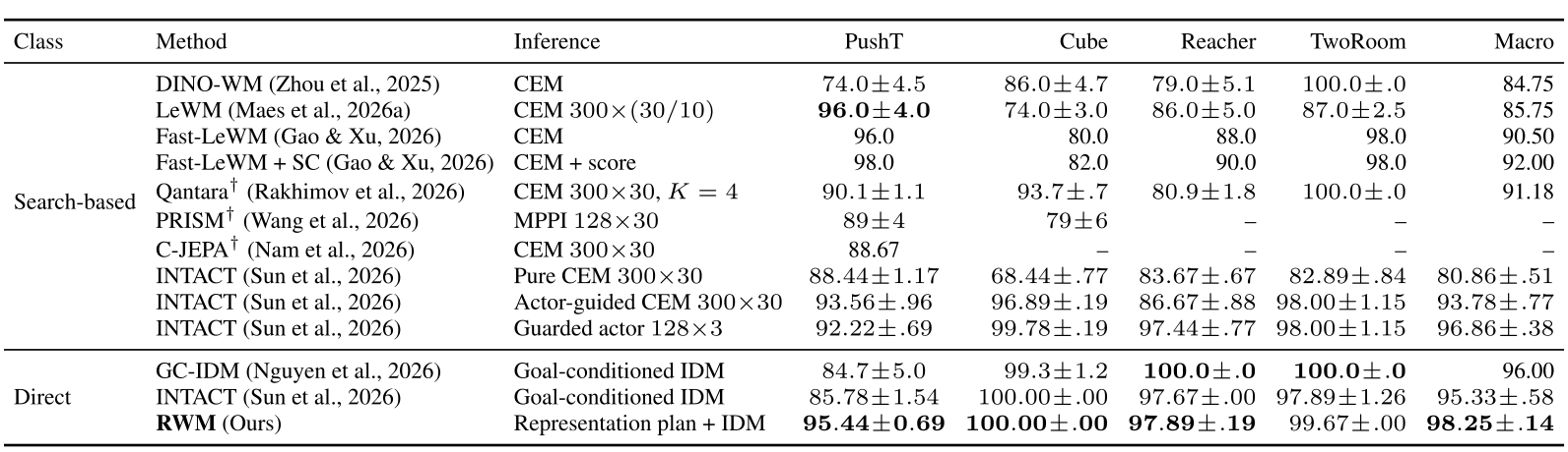
Table 1 distinguishes search-based and direct methods. Published external rows are reference values, not paired controls. Dagger-marked methods use partial task coverage or a distinct reproduction protocol, so a blanket ranking across all rows should not be read as a fully controlled comparison.
LIBERO-Goal setup
The ten LIBERO-Goal tasks follow the RC-aux comparison setting for LeWM, RC-aux, and RWM [19]. OpenVLA-OFT is an external large pretrained reference [18]. Appendix A.2 explains the additional latent-displacement predictor used when the goal image is absent.
4.2 Continuous-control results
RWM reports success of 95.44% on PushT, 100.00% on Cube, 97.89% on Reacher, and 99.67% on TwoRoom, yielding 98.25±0.14% macro success. The strongest matched INTACT variant reaches 96.86±0.38% with guarded actor search; its direct inverse-dynamics variant reaches 95.33±0.58%.
The largest direct-baseline gain is PushT, from 85.78% to 95.44%. The guarded actor evaluates 128×3 candidate trajectories. RWM avoids that search, but operation counts alone do not establish an equivalent wall-clock acceleration.
4.3 LIBERO-Goal results
Table 2 retains every task and model size. The 0.03-billion-parameter RWM adaptation averages 93.0%, compared with 71.2% for LeWM and 81.2% for RC-aux, each listed at 0.07 billion. The external pretrained 7-billion-parameter OpenVLA-OFT reaches 97.0%.
The average improvement is not universal across tasks: on T6, RWM’s 64% is below RC-aux’s 70%. These comparisons also differ in architecture and, for OpenVLA-OFT, pretraining. The table does not provide repeated-seed uncertainty.

4.4 Ablation studies
Unless stated otherwise, ablations use a single training seed, 3072. The reported variations describe that experiment rather than the three-seed uncertainty of the main continuous-control table.
Representations without explicit regularization
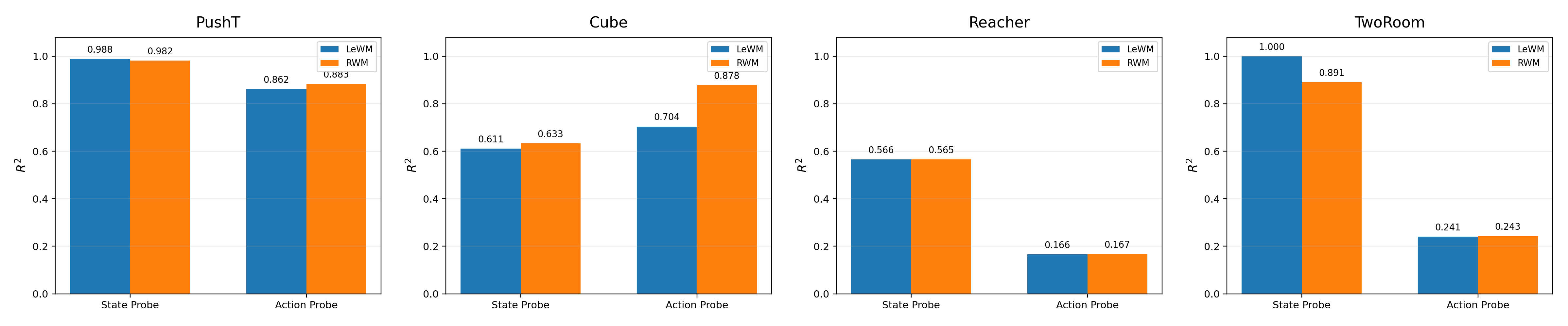
Frozen encoders feed identical tiny MLP probes trained for one epoch. A state probe predicts simulator configuration excluding velocity; an action probe predicts the action from consecutive latent states. Evaluation uses an episode-split validation set and reports R².
Figure 3 shows broadly comparable recoverability to LeWM without an explicit representation regularizer or forward predictor. RWM has lower state recovery on TwoRoom and stronger action recovery on Cube. Probe accuracy is evidence about accessible information, not proof that every planned latent point is physically realizable.
Information in constructed representations
Probes trained only on observed encodings are then evaluated on interpolated representations. State prediction remains close to that from observed encodings; action prediction degrades when one or both inputs are constructed, especially outside the strongest PushT and Cube cases.
Figure 4 preserves all four environments and all action-pair variants. The experiment supports useful transfer of learned state/action information off observed codes. It does not itself execute every decoded trajectory.

Closed-loop interval
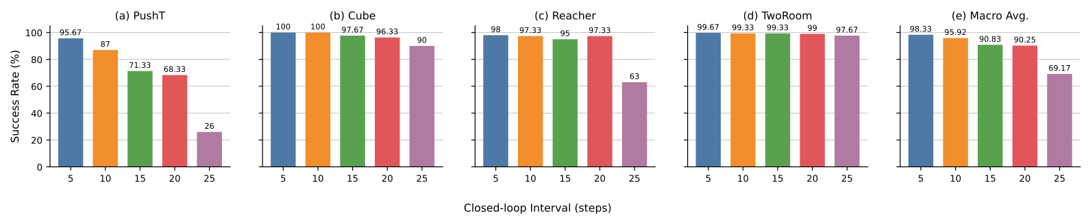
With the model fixed, the study executes 5, 10, 15, 20, or 25 actions before replanning. At five steps, macro success is 98.33%; at twenty-five it falls to 69.17%. PushT drops from 95.67% to 26%, and Reacher from 98% to 63%, while Cube and TwoRoom remain comparatively robust.
The 98.33% ablation value comes from the single-seed setting and differs from the main table’s 98.25% three-seed mean. These results show that feedback is central to the reported performance despite the ability to decode a longer open-loop path.
Role of training objectives
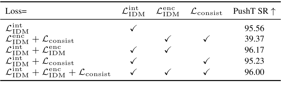
Removing interpolation-based inverse dynamics while retaining the other two terms reduces PushT success from 96.00% to 39.37%. Every tested variant retaining interpolation action supervision scores between 95.23% and 96.17%; the interpolation-only model reaches 95.56%.
The full objective is therefore not the best single-seed success row. The authors favor it for complementary representation properties: encoded-state supervision raises reported state-probe R² from 0.95 to 0.98, while consistency aligns the constructed and observed-state geometries.
5. Conclusion
The study supports action-supervised latent path construction as a useful search-free controller on these simulated benchmarks. Its strongest controlled evidence comes from the matched INTACT comparisons and the loss and feedback ablations.
General feasibility of arbitrary endpoint interpolation, complex multimodal paths, physical-robot deployment, and measured runtime remain unestablished here. The goal-unobserved manipulation extension adds a learned path-construction predictor, so its success should be interpreted separately from fixed endpoint interpolation.
Appendix
The complete appendix is retained: training configuration, the goal-unobserved manipulation architecture, and all four physical-state decoding figure grids.
A.1 Training details
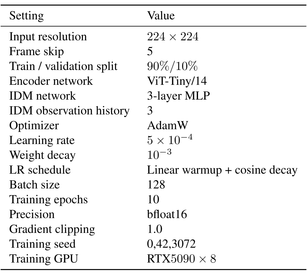
Continuous-control observations are resized to 224×224. A frame skip of five groups low-level actions into blocks. The encoder is ViT-Tiny/14 trained from scratch, and inverse dynamics uses a three-layer MLP. Table 4 preserves the complete configuration, including observation history, optimizer, schedule, precision, clipping, seeds, and hardware.
The encoder training uses a sample-level 90%/10% train/validation split, distinct from the episode-split probe evaluation. AdamW uses learning rate 5×10⁻⁴ and weight decay 10⁻³, with the prose specifying 5×10⁻⁵ for Reacher. Models train for ten epochs at batch size 128 with linear warmup and cosine decay.
A.2 LIBERO-Goal implementation
Because a goal observation is unavailable at test time, an additional predictor learns latent displacements from future demonstration states during training. At inference its predicted displacement replaces the missing endpoint-derived displacement, allowing iterative construction of the next latent state.
This version uses ViT-Small, fuses visual features with proprioception, and conditions both the displacement predictor and inverse dynamics on the task ID. It is a task-conditioned learned extension of RWM, rather than the unchanged goal-observed two-module architecture.
A.3 Physical-state probing visualizations
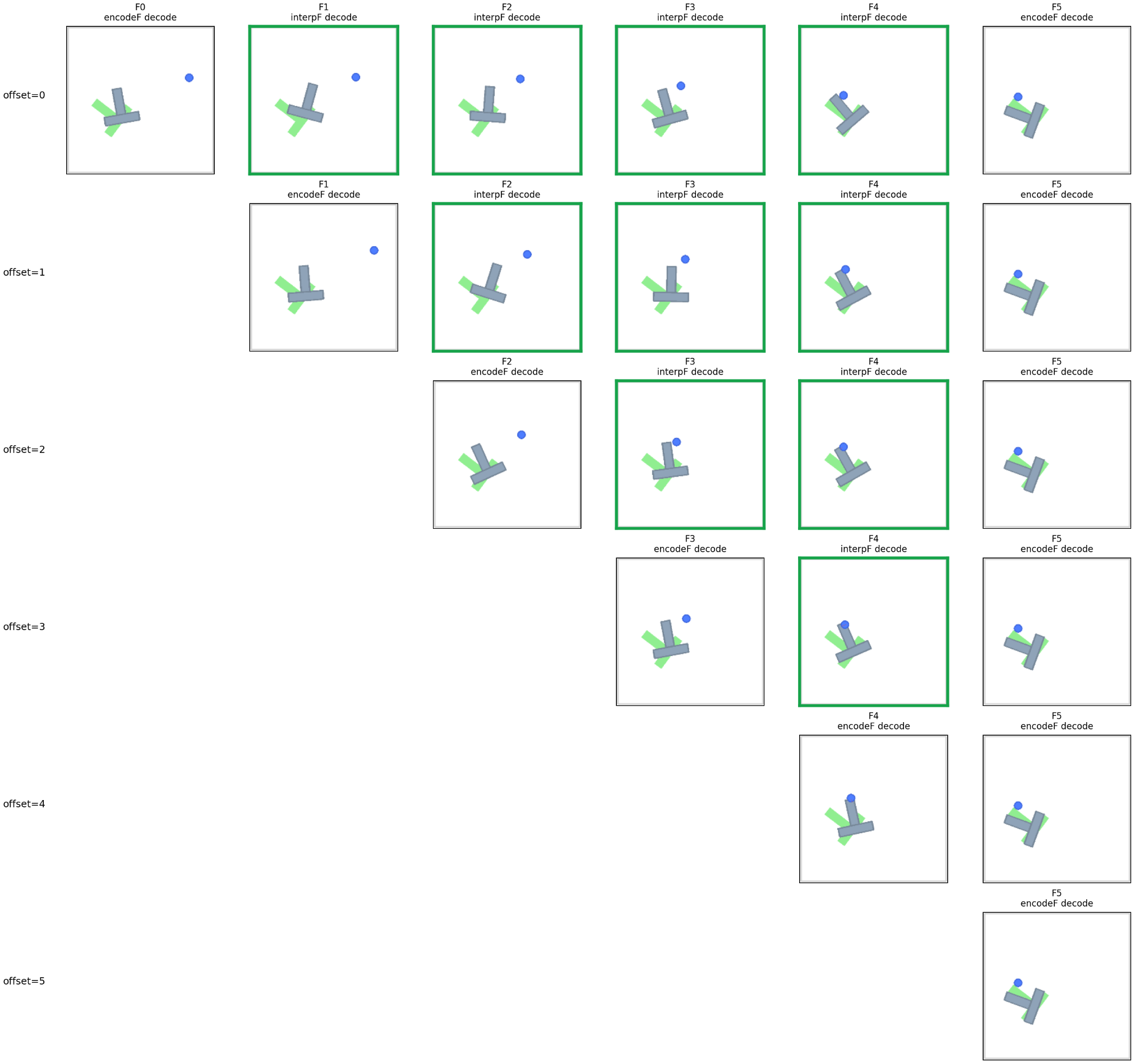
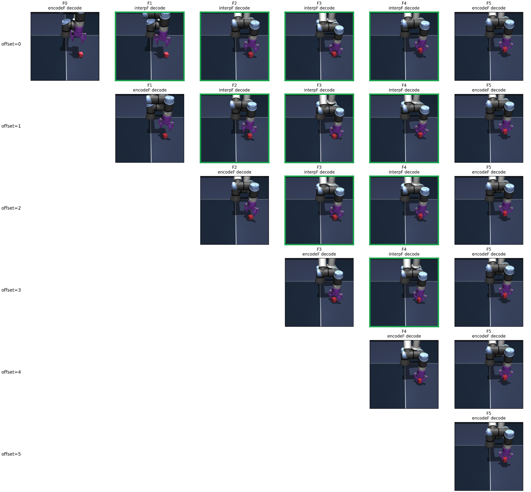
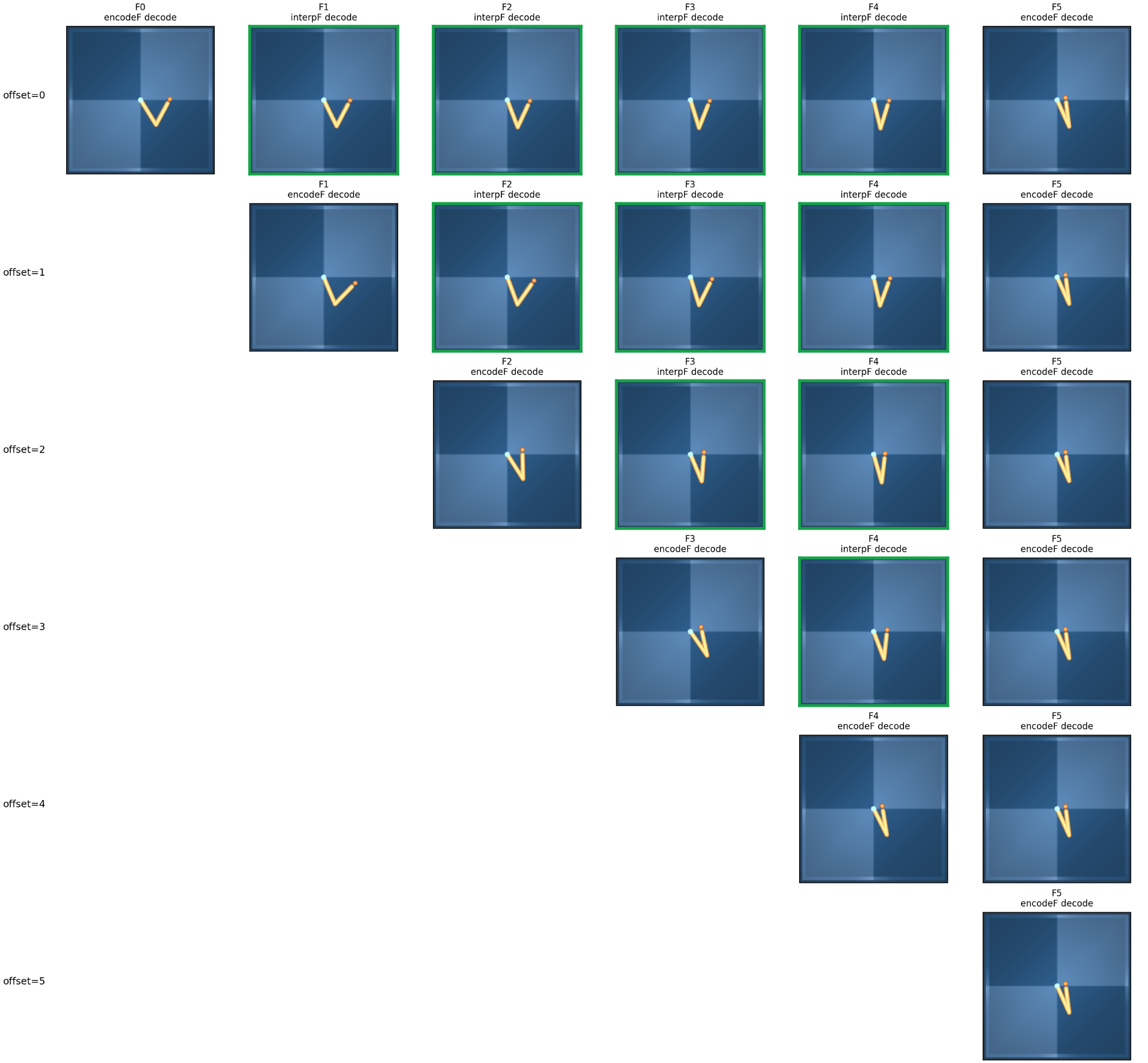
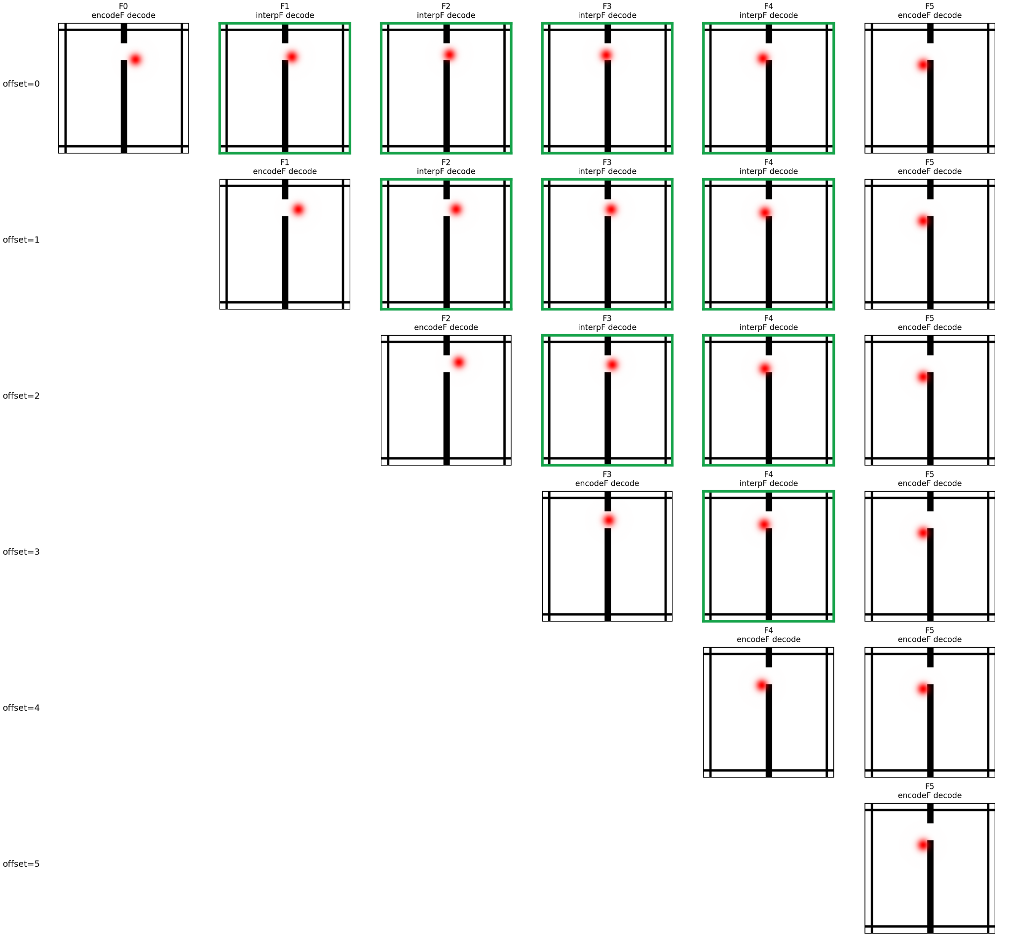
Figures 6–9 retain all state-decoding grids for PushT, Cube, Reacher, and TwoRoom. Black borders denote states decoded from encoded observations; green borders denote states decoded from interpolated codes. These are simulator renderings of probe-predicted physical configurations.
The coherent intermediate configurations are qualitative evidence about latent information. They are not additional successful physical-robot rollouts or a guarantee of action-path feasibility.