Overview


At a glance
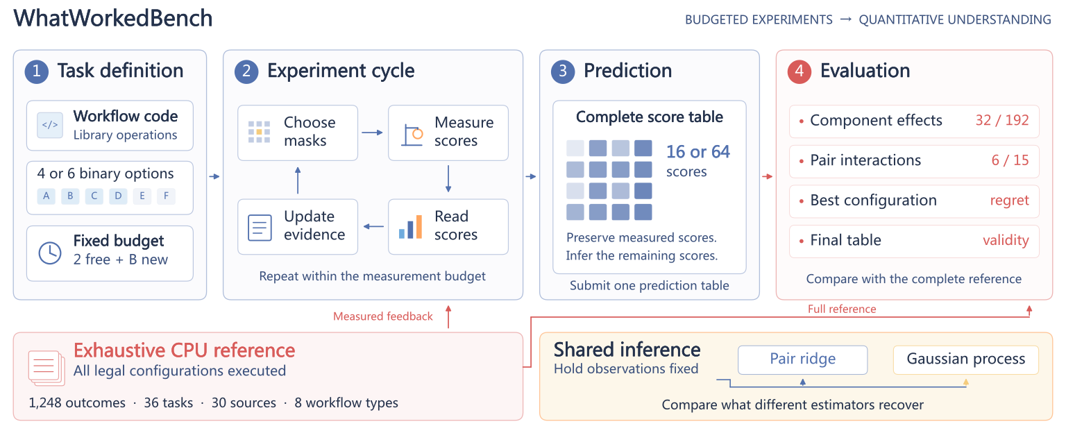
WhatWorkedBench tests whether agents can predict the effects of computational changes after limited experiments, rather than merely find a good configuration. Its exhaustive reference covers 36 task conditions, 30 sources, eight workflow families, and 1,248 configuration records. The main study has 4,206 numerical-control records and 108 agent episodes. Better numerical inference and explicit program equivalences improve reconstruction, but optimization success often leaves large effect errors. Results concern small, fixed, deterministic workflows and dated DeepSeek API cohorts; they do not establish general scientific understanding.
1 Introduction
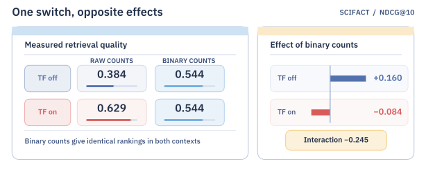
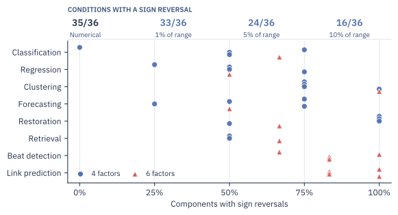
An agent chooses measurements and predicts the entire response surface: one score for every combination of binary options. Conditional effects compare one option with all other settings fixed. They can reverse sign across backgrounds, as SciFact retrieval illustrates. Thirty-five of 36 conditions contain reversals; 24 retain them when both directions exceed 5% of the score range. The benchmark separates measurement selection, numerical reconstruction, and use of program structure. It provides 3,392 conditional effects and 342 mean pair interactions.
2 Related Work
Existing benchmarks assess experimental discovery, research execution, planning, and factorial attribution. This benchmark instead grades the complete numerical effect field against exhaustive native execution. Reconstructing the same observations with different estimators helps separate evidence acquisition from inference. [42], [23], [5], [8], [4], [35].
3 Task and evaluation protocol
Each task has four or six binary options, hence 16 or 64 legal configurations. Two all-off/all-on anchors are free; budget B pays for additional distinct measurements. Repeats are free, and invalid over-budget batches make no partial changes. Agents submit a finite utility in [0,1] for every configuration. Grading restores observed values before scoring, and submission ends the episode. Frozen implementations, seeds, and evaluation cohorts make the reference deterministic.
Primary numerical target.
The primary error is mean absolute error over every conditional component effect: 32 contrasts for four factors and 192 for six. Recovery is max(0, 1 − effect error / mean absolute true effect), with a separate numerical-flatness rule. Zero recovery therefore means error at least as large as the average true effect, not that every prediction is wrong. Complete effects plus one anchor determine all utilities. A maximum per-effect error bound of ε implies at most kε error for a k-option change; average error does not give this guarantee.
Equations 1–2
| (1) |
| (2) |
Additional numerical outputs.
Additional outputs measure mean pair-interaction error, complete-grid error, and regret of the predicted best configuration. Ties favor fewer enabled options, then lexical order. Strict reconstruction requires every effect error to remain within 10% of the task’s score range, subject to a numerical floor. Five tolerances supplement this diagnostic. Missing submissions receive zero recovery, strict credit, and exact-choice credit; their raw errors are undefined.
4 Native catalog and reference validation
Twenty-two original four-factor conditions span classification, regression, clustering, forecasting, restoration, and retrieval. Six paired variants add two options on the same sources; eight more six-factor cases add beat detection and link prediction. The 352 four-factor and 896 six-factor records include 96 repeated original-subcube outcomes. The inventory distinguishes source counts from task conditions and retains shared archive relationships.
| Workflow | Sources | Native operation and metric | ||
|---|---|---|---|---|
| Classification | 4 | 1 | 4 | Logistic regression; balanced accuracy |
| Regression | 4 | 1 | 4 | Ridge regression; transformed MAE |
| Clustering | 4 | 1 | 4 | -means; normalized mutual information |
| Forecasting | 4 | 1 | 4 | One-step ridge forecasts; transformed MAE |
| Restoration | 4 | 1 | 4 | Native image filters; transformed pixel RMSE |
| Retrieval | 2 | 1 | 2 | TF–IDF retrieval; NDCG@10 |
| Beat detection | 0 | 4 | 4 | SciPy signal processing; event F1 |
| Link prediction | 0 | 4 | 4 | NetworkX features and logistic regression; ROC AUC |
| Total | 22 | 14 | 30 | 36 conditions across eight families |
Conditional structure across the catalog.
Requiring reversal magnitudes above 1%, 5%, or 10% of response range leaves 33, 24, or 16 conditions, respectively. These describe the frozen catalog; they are not prevalence estimates for arbitrary scientific experiments.
Data access and native evaluation.
Supervised transforms fit only training data, duplicate feature vectors stay together across splits, and forecasting uses preceding observations. Restoration references and retrieval relevance labels remain evaluation targets. Beat detection uses archived waveforms, while graph features use observed edges and disjoint calibration/test pairs. Appendix C specifies each boundary. [12], [13].
Complete references and reproducible episodes.
Cold replay, independent metric implementations, and target-perturbation checks validate the references. A standalone prepared-input replay reproduces all 1,248 records in a reported 127.87 seconds on one computation thread; the episode engine agrees with 4,206 control records. A trusted host serves cached native outcomes. Measurement credits limit access to information, rather than simulate actual experiment execution costs.
5 Experimental setup
Numerical reference methods.
D1 ridge models additive effects; D2 also includes pair interactions. Sequential designs use their feature geometry, and random D2 averages 20 seeds. Gaussian-process controls fit a Hamming-distance kernel and select measurements to reduce uncertainty in either utilities or conditional effects. Hyperparameters use leave-one-out error. Code-equivalence controls measure representative configurations and propagate predictions across native-verified aliases. [11], [37].
Agents and budgets.
The 108 core episodes comprise 72 four-factor Flash/Pro runs at B=4 or 8 and 36 six-factor Flash full-information/opaque runs at B=20. They use one matched source per original family. Agents have four tools, numerical libraries, two ridge helpers, 20 calculation calls, a 32,768-token output cap, and a 1,800-second deadline. Original and additional September cohorts remain separate because the recorded Flash alias’s provider routing changed. Six completed B=32 submissions on added families form a separate analysis.
Aggregation and delivery.
Scores average repetitions within source, sources within family, then families equally. Four-factor agents deliver 63 of 72 artifacts; all attempts remain in recovery denominators. Original failures involve rate limiting, while later Pro runs also miss deadlines without rate-limit responses. Some later information-study HTTP-success streams deliver no parsed model response. Delivery is scored separately from transport status.
6 Results
6.1 Optimization success and intervention knowledge are distinct targets
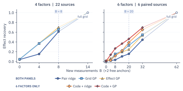
At B=8 across 22 four-factor sources, D2 reaches 0.612 recovery, chooses 15 exact optima, and passes strict reconstruction on three. Thirteen cases choose an optimum while still failing the strict effect threshold. Effect GP reaches 0.701 recovery and 16 optima but only one strict pass. Thus average reconstruction, worst-effect error, and configuration choice rank methods differently. D2 passes on 1, 1, 3, 8, and 20 sources as tolerance rises from 2.5% to 40%. Native-unit evaluation preserves the broad comparison.
6.2 Shared inference extracts additional value from acquired evidence
At B=8, Flash recovery is 0.632 in the original cohort and 0.621 in the additional cohort. Fitting GP to exactly those observations raises the scores to 0.698 and 0.720. This is additional inference, not additional experimentation; the original GP analysis is retrospective, while the additional cohort prespecifies it. Shared fits can also use evidence from episodes without delivered artifacts. In original Flash runs, 67.4% of effects involve unmeasured endpoints, and the submitted predictions outperform same-observation mean completion. Across 18 Flash B=8 episodes, seven choose an exact optimum and one passes strict reconstruction.
| Model | Cohort | Runs | Valid | Recovery | Mean SD | Exact | Strict | |
|---|---|---|---|---|---|---|---|---|
| Flash | Original | 4 | 6 | 6 | 0.178 | — | 2 | 0 |
| Flash | Original | 8 | 12 | 12 | 0.632 | 0.073 | 5 | 1 |
| Pro | Original | 4 | 6 | 4 | 0.043 | — | 2 | 0 |
| Pro | Original | 8 | 6 | 4 | 0.366 | — | 3 | 0 |
| Flash | Additional | 4 | 12 | 12 | 0.375 | 0.105 | 5 | 0 |
| Flash | Additional | 8 | 6 | 6 | 0.621 | — | 2 | 0 |
| Pro | Additional | 4 | 12 | 10 | 0.308 | 0.130 | 2 | 0 |
| Pro | Additional | 8 | 12 | 9 | 0.503 | 0.080 | 6 | 1 |
| Acquisition | Records | Delivered | Shared D1 | Shared D2 | Shared GP |
|---|---|---|---|---|---|
| Flash, original | 12 | 0.632 | 0.604 | 0.550 | 0.698 |
| Pro, original | 6 | 0.366 | 0.628 | 0.567 | 0.692 |
| Flash, additional | 6 | 0.621 | 0.598 | 0.537 | 0.720 |
| Pro, additional | 12 | 0.503 | 0.564 | 0.670 | 0.667 |
| D1 | 6 | 0.546 | 0.546 | 0.592 | 0.592 |
| D2 | 6 | 0.627 | 0.571 | 0.627 | 0.669 |
| Random D2 | 120 | 0.523 | 0.542 | 0.523 | 0.619 |
| GP-G | 6 | 0.666 | 0.564 | 0.633 | 0.666 |
| GP-E | 6 | 0.640 | 0.553 | 0.568 | 0.640 |
6.3 Program structure increases the value of measurements
Across six paired six-factor workflows at B=20, code-equivalence constraints raise D2 recovery from 0.157 to 0.389 and effect GP from 0.248 to 0.462. All four sources with nontrivial classes improve; two identity controls stay unchanged. Simply showing agents full workflow information does not reliably help: full-versus-opaque delivered differences are slightly positive originally and negative later. In eight diagnostic runs, agents report every registered inactive-option rule yet submit ridge tables violating those rules. Offline projection onto equivalence classes increases mean recovery from 0.338 to 0.507 without new observations.
6.4 Shared inference on added workflow families
Six completed Flash B=32 submissions—three beat-detection and three graph sources—improve from 0.303 to 0.455 family-macro recovery after same-observation GP fitting. All six improve. Matched numerical controls reach 0.230 for D2, 0.414 for grid GP, and 0.404 for effect GP. These results condition on successful delivery and are separate from the 108 core episodes.
7 A platform for research on experimental understanding
The public task descriptions, reference surfaces, traces, and exact effects support matched tests of experimental policies, reconstruction methods, and program constraints. Exhaustive grading is feasible because the documented search spaces are finite and small. Generalization to stochastic experiments, open-ended scientific goals, or larger workflows remains outside this evaluation.
8 Conclusion
The evidence supports evaluating what an agent can predict after experimentation alongside the configuration it selects and whether it delivers a usable artifact. Shared GP fitting and executable equivalences expose recoverable errors. Verbal recognition of program rules alone does not ensure numerically consistent predictions.
Reproducibility statement
The authors report standalone reproduction of all 4,206 recorded scores and all 1,248 native configurations. Artifacts retain task semantics, prepared inputs, source manifests, code identities, numerical controls, and audits.
AI use statement
An AI coding assistant contributed across literature exploration, workflow and protocol design, preparation, implementation, analysis, figures, and drafting. DeepSeek models also served as evaluated agents. The authors describe cold replay and independent numerical checks as verification and preserve generated code and analysis records.
Ethics statement
The study uses archived public research data with source-specific terms. ECG tasks measure event detection in stored signal segments; they do not test clinical deployment. A trusted evaluator keeps full reference outcomes separate from agents’ purchased aggregate observations.
Appendix A Benchmark design and related evaluations
The appendices document comparison targets, datasets, preparation boundaries, every workflow option, metrics, numerical methods, agent interfaces, and complete result breakdowns.
Interactive experimental discovery.
Interactive-discovery benchmarks already test hypothesis formation, experimental design, and acquired predictions. WhatWorkedBench’s distinguishing evaluation object is the full conditional-effect field of documented computational interventions; identical observations can be reused to compare reconstruction methods. [42], [5], [23], [24], [25], [6], [19], [43].
| Evaluation | Experimental object | Reference and scored target |
|---|---|---|
| BoxingGym | Generative scientific environments | Information gain, predictive error, and explanation-enabled predictions |
| Gravity-Bench | Gravitational simulations | Numerical discovery answers under an observation budget |
| Science-Gym | Physics and epidemiology simulations | Discovered equations and their predictive behavior |
| SciGym | Biological dynamical systems | Network, reaction, and simulation reconstruction |
| Science sandboxes | Biological experimental loops | Task performance and scientific understanding |
| CAFE | Configurable compound-AI pipelines | Factor effects and interactions from rated outputs |
| petri-bench | Procedurally perturbed simulations | Changed factors, direction, interaction sign, and controlled evidence |
| WhatWorkedBench | Native component interventions | Complete conditional-effect predictions, choice, delivery, and shared reconstruction |
Understanding and attribution.
Science sandboxes separate task success from learning system rules; CAFE attributes factorial component effects; petri-bench scores controlled changes and interaction signs. This benchmark evaluates every conditional effect implied by a submitted numerical table. [18], [4], [33].
Research workflows and scientific tools.
Research-workflow benchmarks score search reports, programs, hypotheses, reproduced experiments, tool use, or scientific outputs. Here, fixed finite workflows allow exhaustive checking of predictions after partial observation. [39], [40], [41], [7], [26], [27], [8], [28], [29], [30], [47], [48], [49], [31], [32].
Planning and learned artifacts.
Ablation-planning and skill-learning evaluations provide related settings, but the delivered knowledge artifact here is a complete numerical response surface backed by executed measurements. [1], [2], [3], [20], [14].
Design and response-surface foundations.
The numerical foundations combine Bayesian experimental design, variance-reduction active learning, GP conditioning, factorial representations, and hyperparameter-importance analysis. Exhaustive outcomes replace surrogate estimates as the grading reference. [35], [36], [37], [11], [34], [9], [10], [38].
Evidence from automated research.
Prior automated-research studies motivate preserving intervention definitions, implementation identities, and trial histories. The Discovery Certification Protocol’s recovery event concerns reaching a target result without its history; WhatWorkedBench’s recovery measures numerical effect accuracy, a different quantity. [15], [21], [16], [17], [22].
Appendix B Source inventory
The complete inventory lists 30 sources with prepared input sizes, scoring cohorts, and four-/six-factor status. Six paired variants reproduce their original E=F=0 subcubes, explaining 96 repeated configuration records rather than additional independent sources.
| Family | Source ID | Prepared input | Evaluation | |
| Classification | banknote | 943 rows 4 | 405 rows | 4 |
| breast_diagnostic | 398 rows 30 | 171 rows | 4 | |
| ionosphere | 245 rows 34 | 105 rows | 4 | |
| spambase | 2,947 rows 57 | 1,263 rows | 4/6 | |
| Regression | airfoil | 1,052 rows 5 | 451 rows | 4 |
| concrete | 702 rows 8 | 303 rows | 4/6 | |
| energy_efficiency | 537 rows 8 | 231 rows | 4 | |
| yacht | 215 rows 6 | 93 rows | 4 | |
| Clustering | dry_bean | 13,543 rows 16 | 7 reference classes | 4 |
| glass | 213 rows 9 | 6 reference classes | 4 | |
| seeds | 210 rows 7 | 3 reference classes | 4 | |
| wine | 178 rows 13 | 3 reference classes | 4/6 | |
| Forecasting | co2 | 1,713 training points | 571 next points | 4/6 |
| elnino | 549 training points | 183 next points | 4 | |
| nile | 75 training points | 25 next points | 4 | |
| sunspots | 231 training points | 78 next points | 4 | |
| Image restoration | astronaut | 256 256 pixels | Clean reference | 4/6 |
| coffee | 171 256 pixels | Clean reference | 4 | |
| hubble_deep_field | 223 256 pixels | Clean reference | 4 | |
| rocket | 171 256 pixels | Clean reference | 4 | |
| Retrieval | arguana | 8,567 documents | 64 queries | 4 |
| scifact | 5,183 documents | 64 queries | 4/6 | |
| Beat detection | mitdb_100 | 108,000 at 360 Hz | 369 interior events | 6 |
| mitdb_101 | 108,000 at 360 Hz | 340 interior events | 6 | |
| mitdb_102 | 108,000 at 360 Hz | 364 interior events | 6 | |
| mitdb_103 | 108,000 at 360 Hz | 352 interior events | 6 | |
| Link prediction | graph_adjnoun | 112 nodes, 255 edges | 170 cal., 170 test | 6 |
| graph_dolphins | 62 nodes, 95 edges | 64 cal., 64 test | 6 | |
| graph_football | 115 nodes, 367 edges | 246 cal., 246 test | 6 | |
| graph_lesmis | 77 nodes, 152 edges | 102 cal., 102 test | 6 |
Source terms and attribution.
Source manifests preserve dataset-specific attribution and terms for UCI, statsmodels, scikit-image, SciFact, ArguAna, MIT-BIH, and the graph archive. Shared collections and paired variants are retained in source accounting; source count should not be read as complete statistical independence.
Appendix C Data preparation and evaluation boundaries
C.1 Tabular classification, regression, and clustering
Tabular preparation removes duplicate feature–label rows and groups identical feature vectors before a fixed 70/30 supervised split. Feature transforms and models fit training data only; Energy Efficiency’s second target is excluded. Clustering uses all deduplicated features, fixes cluster count from the known class count, and evaluates agreement with archived labels using NMI.
C.2 Chronological forecasting
Forecasting uses a chronological 75% training prefix. Missing values use only preceding finite observations; CO2 has 59 replacements. All designs fit from index 12 and then make one-step predictions from realized preceding values with fixed parameters. Differenced predictions are restored to levels before any inverse logarithmic transform.
C.3 Image preparation and restoration
Images become grayscale thumbnails with maximum dimension 256. Fixed-seed Gaussian noise of standard deviation 0.1 is added and clipped; every mask receives the same noisy image. Clean pixels enter only evaluator RMSE.
C.4 Retrieval corpora and query cohorts
SciFact and ArguAna each use 64 fixed original queries with source relevance labels. Vectorizers fit sorted corpus documents, and stable ranking breaks ties. ArguAna excludes corpus text identical to each query under every mask, with additional split audits. [50].
C.5 Archived signal records
Four MIT-BIH records contribute five-minute channel-zero segments at 360 Hz. Scoring uses interior events from 1 to 299 seconds, matched one-to-one within 100 ms, with 50/150-ms sensitivity checks. Forward–backward filtering is offline: the task evaluates localization in archived segments, not causal real-time detection.
C.6 Graph construction and pair partitions
Graphs become simple, undirected, and unweighted. Fixed seeds divide edges approximately 60/20/20 into observed, calibration, and test sets. Balanced, disjoint negative pairs accompany calibration and test positives. Every feature uses the same observed graph; logistic regression fits calibration labels and test labels supply ROC AUC.
Appendix D Workflow options and fixed numerical settings
The original four-factor track uses bits A–D; paired variants retain those settings and add E/F. All masks are legal. The tables preserve both settings for all 48 options across eight workflows.
D.1 Classification
Classification applies optional signed logarithms, scaling, class weighting, regularization, feature selection, and PCA before logistic regression. Training-fitted scaling precedes selection and PCA; the fixed solver and seeds are shared across masks.
| Bit | Setting 0 | Setting 1 |
|---|---|---|
| A | Original features | |
| B | Original feature scale | Training-fitted standard scaling |
| C | Uniform class weights | Balanced class weights |
| D | Logistic regression | Logistic regression |
| E | All input features | Training-fitted ANOVA selection at the 50th percentile |
| F | Input representation | PCA retaining 95% variance after optional selection |
D.2 Regression
Regression varies target transformation, scaling, polynomial features, and ridge regularization. E changes polynomial interactions only when C enables polynomial features; F changes scaler type only when B enables scaling. These guards create exact equivalences.
| Bit | Setting 0 | Setting 1 |
|---|---|---|
| A | Original target | Training-target log1p with expm1 inverse |
| B | Original feature scale | Training-fitted feature scaling |
| C | Original features | Degree-two polynomial features without a bias column |
| D | Ridge | Ridge |
| E | Full degree-two polynomial terms | Interaction-only polynomial terms when C is enabled |
| F | Standard scaling when B is enabled | Robust scaling when B is enabled |
D.3 Clustering
Clustering varies feature transforms, scaling, PCA, initialization count/type, and whitening. Whitening is inactive without PCA. K-means uses the known class count, Lloyd updates, and a fixed seed.
| Bit | Setting 0 | Setting 1 |
|---|---|---|
| A | Original features | Signed logarithmic feature transform |
| B | Original feature scale | Feature-only standard scaling |
| C | All input features | PCA retaining 95% variance |
| D | One k-means initialization | Ten k-means initializations |
| E | Unwhitened PCA coordinates | Whitened coordinates when C is enabled |
| F | K-means++ initialization | Random initialization |
D.4 Forecasting
Forecast options cover trend, lag count, level transform, ridge regularization, scaler type, and differencing. Fitting starts at the same time index for every mask; inversion restores levels before undoing the logarithm.
| Bit | Setting 0 | Setting 1 |
|---|---|---|
| A | Lag features | Lag features and a linear time trend |
| B | Lag 1 | Lags 1 through 12 |
| C | Original series levels | log1p levels with expm1 inverse |
| D | Ridge | Ridge |
| E | Training-fitted standard scaling | Training-fitted robust scaling |
| F | Model series levels | Model first differences and restore the previous level |
D.5 Image restoration
Restoration applies median, Gaussian, Wiener, and unsharp filters in fixed order before clipping. Gaussian width is inactive without its filter, and median width is inactive without the median filter; these generate equivalent configurations.
| Bit | Setting 0 | Setting 1 |
|---|---|---|
| A | Pass the image onward | Median filter with a window |
| B | Pass the image onward | Gaussian filter with |
| C | Pass the image onward | Wiener filter with a neighborhood |
| D | Pass the image onward | Unsharp mask with Gaussian , amount 0.5 |
| E | Gaussian when B is enabled | Gaussian when B is enabled |
| F | Median window when A is enabled | Median window when A is enabled |
D.6 Retrieval
Retrieval varies n-grams, stopword removal, sublinear TF, IDF, binary counts, and vector normalization. Corpus-fitted vectors produce dot-product rankings. Binary counts disable the effect of the sublinear transform, explaining the introductory reversal example.
| Bit | Setting 0 | Setting 1 |
|---|---|---|
| A | Unigrams | Unigrams and bigrams |
| B | Retain stopwords | Remove the scikit-learn English stopword set |
| C | Raw term frequency | Sublinear term frequency |
| D | Unit term weights | Inverse-document-frequency weighting |
| E | Frequency counts | Binary term counts |
| F | L2 vector normalization | Unnormalized document and query vectors |
D.7 Beat detection
Beat detection varies high-/low-pass filtering, envelope construction, moving integration, thresholding, and minimum peak distance. Robust thresholds use scaled MAD; peaks align within 75 ms to maximal absolute filtered amplitude and duplicates merge.
| Bit | Setting 0 | Setting 1 |
|---|---|---|
| A | Median-centered waveform | Additional second-order 0.5-Hz high-pass filter |
| B | Current waveform | Additional second-order 35-Hz low-pass filter |
| C | Absolute-amplitude envelope | Squared first-difference envelope |
| D | Current envelope | 120-ms moving integration |
| E | Mean plus one standard deviation | Median plus three scaled MAD units |
| F | 200-ms minimum peak distance | 300-ms minimum peak distance |
D.8 Link prediction
Link prediction toggles five graph-neighborhood scores and feature scaling. With every score disabled, a zero column yields an intercept-only classifier. Calibration-fitted logistic probabilities provide test ranking scores.
| Bit | Setting 0 | Setting 1 |
|---|---|---|
| A | Feature absent | Common-neighbor count |
| B | Feature absent | Jaccard coefficient |
| C | Feature absent | Adamic–Adar index |
| D | Feature absent | Resource-allocation index |
| E | Feature absent | Preferential-attachment score |
| F | Original feature scales | Calibration-fitted standard scaling |
Appendix E Response scales and conditional structure
The table retains each family’s response-range and mean-effect intervals. Recovery normalizes by mean absolute true effect, so a similar raw prediction error can produce very different recovery across sources. Source-specific raw errors and utility scales accompany the aggregate scores.
| Workflow | Conditions | Score range | Mean effect |
|---|---|---|---|
| Regression | 5 | 0.0402–0.3847 | 0.0096–0.1018 |
| Retrieval | 3 | 0.3094–0.6394 | 0.0755–0.0992 |
| Image restoration | 5 | 0.1928–0.3306 | 0.0401–0.0678 |
| Classification | 5 | 0.0364–0.2799 | 0.0081–0.0391 |
| Forecasting | 5 | 0.0109–0.1594 | 0.0026–0.0384 |
| Clustering | 5 | 0.1733–0.8203 | 0.0433–0.1362 |
| Beat detection | 4 | 0.4464–0.6268 | 0.0538–0.1299 |
| Link prediction | 4 | 0.2470–0.4035 | 0.0199–0.0366 |
Appendix F Metric definitions and artifact grading
F.1 Coverage of joint interventions
Telescoping component changes reconstruct any joint intervention. A predicted response table enforces path consistency automatically. The maximum-error guarantee applies to every traversed edge, while mean error and average pair interactions can conceal large or oppositely signed effects.
Equation 3
| (3) |
F.2 Configuration choice and effect recovery
The two-bit counterexample preserves both free anchors and the unique best configuration while recovery approaches zero. Adding inactive bits embeds it into either benchmark track, demonstrating that correct optimization does not imply correct intervention knowledge.
| Configuration | 00 | 10 | 01 | 11 |
|---|---|---|---|---|
| True utility | 0 | 1 | 0 | 0 |
| Predicted utility | 0 | 1 | 0 |
F.3 Native metrics and utility transformations
Utilities use balanced accuracy, NMI, NDCG, event F1, or ROC AUC directly. Regression, forecasting, and restoration costs become bounded utilities through a reversible scale transformation; scales derive from training-target interquartile ranges or the fixed image-noise scale. Independent event matching checks the native matcher.
Equations 4–5
| (4) |
| (5) |
F.4 Effect, interaction, and grid errors
Pair-interaction MAE averages second-difference errors; grid MAE compares all predicted utilities. Unobserved-cell error is also retained. Exact-choice credit uses a numerical tolerance of 10⁻¹², while a separate near-optimal flag allows 0.02 utility and marks tasks whose full range is smaller.
Equation 6
| (6) |
F.5 Artifact validation and the strict diagnostic
Artifacts must have exactly one finite [0,1] value per legal mask; duplicate keys, Booleans, missing cells, and extra masks fail. Measured values are restored before grading. Failed delivery receives zero headline credit, but shared estimators may still reconstruct from observations already acquired.
Equation 7
| (7) |
F.6 Measured effects and remaining reconstruction
Effects with two observed endpoints are exact after restoration; remaining error comes from contrasts involving unmeasured cells. A same-observation mean-fill baseline distinguishes this direct knowledge from reconstruction. Original Flash B=8 has 32.6% known edges: agent recovery is 0.632 versus 0.287 for mean fill, and shared GP reaches 0.698. The retrospective coverage analysis includes 94 valid core artifacts; some appendix rows condition on validity and therefore differ from all-attempt headline averages.
Equation 8
| (8) |
| Setting | Valid | Known edges | ||||||
|---|---|---|---|---|---|---|---|---|
| O, 4 factors | 4 | 6 | 6 | 10.4% | 0.056 | 0.178 | 1.093 | 0.921 |
| O, 4 factors | 8 | 12 | 6 | 32.6% | 0.287 | 0.632 | 1.054 | 0.542 |
| O, 6 factors, full | 20 | 6 | 6 | 6.8% | 0.012 | 0.268 | 1.156 | 0.824 |
| O, 6 factors, opaque | 20 | 6 | 6 | 14.9% | 0.011 | 0.257 | 1.183 | 0.899 |
| A, 4 factors | 4 | 12 | 6 | 9.9% | 0.084 | 0.375 | 1.075 | 0.710 |
| A, 4 factors | 8 | 6 | 6 | 32.3% | 0.213 | 0.621 | 1.156 | 0.567 |
| A, 6 factors, full | 20 | 10 | 6 | 8.6% | 0.014 | 0.211 | 1.200 | 0.882 |
| A, 6 factors, opaque | 20 | 9 | 6 | 8.8% | 0.028 | 0.283 | 1.172 | 0.790 |
Appendix G Numerical estimators and measurement policies
G.1 Main-effect and pair-effect ridge
D1 fits centered-bit main effects; D2 adds pair products. Ridge selects among five penalties by leave-one-out squared error, leaves the intercept unpenalized, clips predictions, and restores measurements. Sequential design maximizes feature uncertainty without using observed utility values in acquisition. Random D2 samples without replacement across 20 fixed seeds.
Equations 9–10
| (9) |
| (10) |
G.2 Gaussian-process controls
The GP uses an exponential Hamming-distance kernel with an estimated constant mean. Leave-one-out error selects length scale and nugget; the nugget regularizes deterministic data. Grid and effect acquisition reduce posterior uncertainty in utilities or their linear contrasts. Hyperparameters refit after each measurement, and lexical rules resolve ties.
Equations 11–12
| (11) |
| (12) |
G.3 Program-equivalence controls
Native-verified guards reduce 64 masks to 64, 36, 48, 64, 36, and 48 equivalence classes across the six original families. Controls query representatives and distinguish paid measurements from inferred aliases. Once every class is observed, they stop spending even when the allowed budget remains.
G.4 Shared estimators and aggregation
Shared estimators fit exactly each episode’s acquired set, without running their own acquisition policy. Random seeds and repeated episodes average within source; sources average within family; participating families receive equal weight. Agent comparisons use the same six sources, while full numerical controls use their stated larger catalogs.
Appendix H Agent interface and execution environment
Four tools expose evidence, purchase configurations, run numerical Python, and submit predictions or a named ridge helper. Each calculation uses a fresh restricted process with public data and observations; network and bundled dataset labels are unavailable. Calls allow 30 CPU seconds and 45 wall seconds, with 20 calls per episode. The interface exposes remaining time and recommends submission with 120 seconds left. Full/opaque six-factor views share utility-only receipts but differ jointly in code, option semantics, source identity, and input summaries.
Appendix I Recorded prompts and task payloads
The appendix identifies frozen system/prompt templates and task payloads in the companion bundle; it does not reproduce full prompt listings. Templates request all 16/64 predictions, disclose budgets and deadlines, and allow explicit ridge-helper submission. The structure probe adds a first-call rule report in both arms and supplies verified rules only in one.
Appendix J Study design and execution accounting
Construction and analysis order.
Catalog extensions were specified before their native outcomes. Initial ridge results preceded GP and equivalence analyses. Original-cohort shared GP is retrospective; later information and additional-agent studies followed inspection of earlier results. The additional 66-episode plan retained prompts, budgets, and deadlines, with API identifiers and dates reported separately. This chronology limits treating every comparison as an independent preregistered confirmation.
Budgets and records.
The 4,206 controls comprise 1,936 four-factor ridge/design, 924 paired ridge/design, 84 equivalence-ridge, 302 GP, and 960 added-source records. The execution table separately lists 108 core and eight structure-diagnostic episodes. Every attempted provider episode remains; five administrative records with zero requests are excluded. Rate limits, deadline failures, empty HTTP-success streams, and a scheduling amendment are documented rather than silently removed.
| Agent study | Episodes | Valid | HTTP 429 | ||
|---|---|---|---|---|---|
| Flash and Pro original cohort | 4 | 4, 8 | 24 | 20 | 75 |
| Flash full/opaque information | 6 | 20 | 12 | 12 | 0 |
| Flash additional trial | 4 | 8 | 6 | 6 | 0 |
| Additional Flash and Pro | 4 | 4, 8 | 42 | 37 | 0 |
| Additional Flash information | 6 | 20 | 24 | 19 | 0 |
| Structure diagnostic | 6 | 20 | 8 | 8 | 0 |
Appendix K Episode results and paired comparisons
The cohort table preserves delivery denominators and zero recovery for failures. The companion index links all 108 core episodes to measurements, predictions, helper choices, and execution metadata.
| Model | Original episodes | Additional episodes | |||
|---|---|---|---|---|---|
| Valid / runs | Valid / runs | ||||
| Flash | 4 | 6/6 | 0.178 | 12/12 | 0.375 |
| Flash | 8 | 12/12 | 0.632 | 6/6 | 0.621 |
| Pro | 4 | 4/6 | 0.043 | 10/12 | 0.308 |
| Pro | 8 | 4/6 | 0.366 | 9/12 | 0.503 |
K.1 Information supplied to the agent
Full and opaque conditions match sources, budgets, tools, receipts, and deadlines. Full information adds several kinds of workflow information together. Full-minus-opaque delivered recovery is +0.0103 originally and −0.0491 later; shared-GP differences are −0.0242 and −0.0638. Valid-pair-only summaries are conditional analyses, distinct from the all-attempt comparison.
| Cohort | Source | Valid pairs | Delivered | Shared GP | ||||
|---|---|---|---|---|---|---|---|---|
| Full | Opaque | Full | Opaque | |||||
| O | astronaut | 1/1 | 0.294 | 0.255 | +0.039 | 0.379 | 0.137 | +0.242 |
| O | co2 | 1/1 | 0.244 | 0.049 | +0.196 | 0.263 | 0.131 | +0.133 |
| O | concrete | 1/1 | 0.298 | 0.642 | -0.343 | 0.796 | 0.847 | -0.051 |
| O | scifact | 1/1 | 0.522 | 0.407 | +0.115 | 0.598 | 0.468 | +0.130 |
| O | spambase | 1/1 | 0.000 | 0.000 | +0.000 | 0.000 | 0.389 | -0.389 |
| O | wine | 1/1 | 0.247 | 0.191 | +0.056 | 0.205 | 0.414 | -0.209 |
| A | astronaut | 1/2 | 0.275 | 0.000 | +0.275 | 0.217 | 0.112 | +0.105 |
| A | co2 | 1/2 | 0.129 | 0.102 | +0.027 | 0.262 | 0.161 | +0.101 |
| A | concrete | 2/2 | 0.505 | 0.754 | -0.249 | 0.771 | 0.843 | -0.072 |
| A | scifact | 1/2 | 0.153 | 0.357 | -0.204 | 0.300 | 0.496 | -0.195 |
| A | spambase | 2/2 | 0.042 | 0.000 | +0.042 | 0.039 | 0.203 | -0.164 |
| A | wine | 1/2 | 0.006 | 0.193 | -0.187 | 0.002 | 0.160 | -0.158 |
K.2 Repeated high-budget agent runs
Original Flash B=8 has two repetitions per source; the additional cohort has one. Original recovery is 0.6321 and shared GP 0.6976, with five exact choices and one strict pass across 12 episodes. Six additional episodes yield 0.6211 and 0.7205, two exact choices, and no strict passes. Source-level improvements are not universal.
| Source | Flash, original | Flash, additional | Designed D2 | ||
|---|---|---|---|---|---|
| Delivered (SD) | Shared GP | Delivered (SD) | Shared GP | ||
| astronaut | 0.356 (0.144) | 0.645 | 0.270 (—) | 0.523 | 0.634 |
| co2 | 0.365 (0.026) | 0.505 | 0.569 (—) | 0.667 | 0.400 |
| concrete | 0.853 (0.011) | 0.877 | 0.842 (—) | 0.913 | 0.888 |
| scifact | 0.803 (0.096) | 0.799 | 0.762 (—) | 0.761 | 0.799 |
| spambase | 0.637 (0.066) | 0.667 | 0.684 (—) | 0.683 | 0.508 |
| wine | 0.778 (0.095) | 0.691 | 0.599 (—) | 0.775 | 0.533 |
K.3 Structure recognition and application
Eight September 22 diagnostic runs pair code-only and code-plus-rules on four sources. Both arms correctly report all six registered rules, but all final tables use public ridge helpers and violate equivalences. Supplied rules improve three sources and worsen one. Post-hoc class projection preserves acquired observations, reduces raw effect error in every run, raises recovery in seven, and leaves all strict scores at zero. The elicited reporting task and small paired sample qualify this result.
| Source | Information | Rules | Redundant | Equiv. error | Recovery | Post-hoc |
|---|---|---|---|---|---|---|
| concrete | Code | 2/2 | 0/20 | 4.88% | 0.680 | 0.823 |
| concrete | Code + rules | 2/2 | 0/20 | 10.21% | 0.646 | 0.748 |
| wine | Code | 1/1 | 0/20 | 16.97% | 0.000 | 0.000 |
| wine | Code + rules | 1/1 | 0/20 | 15.54% | 0.213 | 0.290 |
| astronaut | Code | 2/2 | 2/20 | 16.77% | 0.000 | 0.415 |
| astronaut | Code + rules | 2/2 | 0/20 | 12.14% | 0.334 | 0.745 |
| scifact | Code | 1/1 | 0/20 | 8.89% | 0.308 | 0.485 |
| scifact | Code + rules | 1/1 | 0/20 | 1.39% | 0.524 | 0.549 |
Appendix L Sensitivity and additional-workflow results
L.1 Sensitivity to individual sources
Same-observation GP improves four sources and worsens two in each Flash cohort. Its mean advantage remains positive after omitting any one source: +0.021 to +0.096 originally and +0.069 to +0.120 later. Equivalence controls improve all four nontrivial sources and leave identity controls unchanged. Omission ranges describe catalog sensitivity, not confidence intervals.
| Comparison | Mean | Median | Source omission range | |||
|---|---|---|---|---|---|---|
| Shared GP, Flash original | 8 | +0.066 | +0.028 | 4 / 0 / 2 | +0.021 | +0.096 |
| Shared GP, Flash additional | 8 | +0.099 | +0.085 | 4 / 0 / 2 | +0.069 | +0.120 |
| Code GP over GP | 20 | +0.214 | +0.166 | 4 / 2 / 0 | +0.121 | +0.257 |
| Code D2 over D2 | 20 | +0.233 | +0.231 | 4 / 2 / 0 | +0.167 | +0.279 |
| Code GP over GP | 32 | +0.159 | +0.131 | 4 / 2 / 0 | +0.096 | +0.191 |
| Code D2 over D2 | 32 | +0.205 | +0.136 | 4 / 2 / 0 | +0.113 | +0.246 |
L.2 Strict-error tolerances
The complete tolerance profile scores identical predictions at maximum-error thresholds from 2.5% to 40%. D2 at B=8 passes three of 22 four-factor sources at 10% but eight at 20%, while retaining the same 15 exact choices. Strict counts should therefore be interpreted alongside continuous recovery and response scales.
| Track | Method | Strict count at tolerance | Exact | |||||||
|---|---|---|---|---|---|---|---|---|---|---|
| .025 | .05 | .10 | .20 | .40 | ||||||
| 4 factors | D1 | 8 | 22 | 0 | 1 | 1 | 5 | 13 | 15 | 0.618 |
| 4 factors | D2 | 8 | 22 | 1 | 1 | 3 | 8 | 20 | 15 | 0.634 |
| 4 factors | GP-G | 8 | 22 | 1 | 1 | 2 | 10 | 19 | 15 | 0.669 |
| 4 factors | GP-E | 8 | 22 | 1 | 1 | 1 | 12 | 19 | 16 | 0.717 |
| 6 factors | D1 | 8 | 6 | 0 | 0 | 0 | 0 | 1 | 2 | 0.405 |
| 6 factors | D2 | 8 | 6 | 0 | 0 | 0 | 0 | 0 | 0 | — |
| 6 factors | GP-G | 8 | 6 | 0 | 0 | 0 | 1 | 1 | 0 | — |
| 6 factors | GP-E | 8 | 6 | 0 | 0 | 0 | 0 | 2 | 0 | — |
| 6 factors | Code D1 | 8 | 6 | 0 | 0 | 0 | 1 | 1 | 2 | 0.063 |
| 6 factors | Code D2 | 8 | 6 | 0 | 0 | 0 | 0 | 0 | 1 | 0.000 |
| 6 factors | Code GP-E | 8 | 6 | 0 | 0 | 0 | 1 | 1 | 2 | 0.544 |
| 6 factors | D1 | 32 | 6 | 0 | 0 | 0 | 1 | 2 | 2 | 0.431 |
| 6 factors | D2 | 32 | 6 | 0 | 0 | 1 | 1 | 2 | 2 | 0.598 |
| 6 factors | GP-G | 32 | 6 | 0 | 0 | 1 | 1 | 4 | 2 | 0.682 |
| 6 factors | GP-E | 32 | 6 | 0 | 0 | 1 | 1 | 4 | 2 | 0.704 |
| 6 factors | Code D1 | 32 | 6 | 0 | 2 | 2 | 3 | 3 | 3 | 0.786 |
| 6 factors | Code D2 | 32 | 6 | 1 | 1 | 3 | 3 | 3 | 2 | 0.987 |
| 6 factors | Code GP-E | 32 | 6 | 1 | 2 | 2 | 3 | 4 | 3 | 0.925 |
L.3 Native-unit sensitivity
Inverse utility transforms regrade the same predictions in native units; all 3,246 original control records have finite inverses. Four-factor B=8 D2 recovery changes from 0.612 to 0.633, and effect GP from 0.701 to 0.712. Program-equivalence gains persist. Random-design strict counts include all seeds, so their denominators differ from source counts.
| Track | Method | Utility | Native | Native strict | ||
|---|---|---|---|---|---|---|
| 4 factors | D1 | 8 | 22 | 0.571 | 0.562 | 1/22 |
| 4 factors | D2 | 8 | 22 | 0.612 | 0.633 | 3/22 |
| 4 factors | Random D2 | 8 | 22 | 0.503 | 0.505 | 14/440 |
| 4 factors | GP-G | 8 | 22 | 0.661 | 0.669 | 2/22 |
| 4 factors | GP-E | 8 | 22 | 0.701 | 0.712 | 2/22 |
| 6 factors | D1 | 20 | 6 | 0.192 | 0.197 | 0/6 |
| 6 factors | D2 | 20 | 6 | 0.157 | 0.171 | 0/6 |
| 6 factors | Random D2 | 20 | 6 | 0.214 | 0.216 | 0/120 |
| 6 factors | GP-G | 20 | 6 | 0.330 | 0.334 | 0/6 |
| 6 factors | GP-E | 20 | 6 | 0.248 | 0.252 | 0/6 |
| 6 factors | Code D1 | 20 | 6 | 0.303 | 0.296 | 1/6 |
| 6 factors | Code D2 | 20 | 6 | 0.389 | 0.384 | 1/6 |
| 6 factors | Code GP-E | 20 | 6 | 0.462 | 0.468 | 1/6 |
| 6 factors | D1 | 32 | 6 | 0.298 | 0.301 | 0/6 |
| 6 factors | D2 | 32 | 6 | 0.445 | 0.451 | 1/6 |
| 6 factors | Random D2 | 32 | 6 | 0.465 | 0.466 | 17/120 |
| 6 factors | GP-G | 32 | 6 | 0.548 | 0.547 | 1/6 |
| 6 factors | GP-E | 32 | 6 | 0.537 | 0.538 | 1/6 |
| 6 factors | Code D1 | 32 | 6 | 0.545 | 0.545 | 2/6 |
| 6 factors | Code D2 | 32 | 6 | 0.650 | 0.650 | 3/6 |
| 6 factors | Code GP-E | 32 | 6 | 0.697 | 0.697 | 2/6 |
L.4 Magnitude of conditional reversals
A reversal needs positive and negative background effects exceeding the same floor. At the numerical floor, 121 of 172 components reverse across 35 conditions and 29 distinct sources. At 5% of response range, this becomes 59 components, 24 conditions, and 20 sources; paired variants merge for source counting.
| Effect floor | Components / 172 | Conditions / 36 | Sources / 30 |
|---|---|---|---|
| utility | 121 | 35 | 29 |
| 1% of response range | 98 | 33 | 28 |
| 5% of response range | 59 | 24 | 20 |
| 10% of response range | 31 | 16 | 14 |
L.5 Signal and graph workflows
All eight added beat/graph sources retain exhaustive references and budget curves. Their higher-order variance quantifies interactions beyond pairs. At B=20, two-family recovery is only 0.0439 for D2 and 0.0435 for effect GP; sparse measurements leave substantial reconstruction error even though exhaustive endpoints are available for validation.
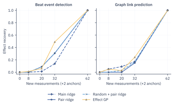
| Source | Min | Max | Sign reversals | Order variance |
|---|---|---|---|---|
| mitdb_100 | 0.502 | 1.000 | 4 | 0.162 |
| mitdb_101 | 0.369 | 0.996 | 6 | 0.140 |
| mitdb_102 | 0.554 | 1.000 | 5 | 0.386 |
| mitdb_103 | 0.506 | 1.000 | 5 | 0.153 |
| graph_lesmis | 0.500 | 0.903 | 6 | 0.419 |
| graph_adjnoun | 0.500 | 0.747 | 5 | 0.084 |
| graph_football | 0.500 | 0.892 | 5 | 0.265 |
| graph_dolphins | 0.500 | 0.764 | 6 | 0.432 |
L.6 Completed agent predictions on the added families
This table conditions on six completed B=32 Flash artifacts, three per added family. Same-observation GP improves each and raises family-macro recovery from 0.303 to 0.455. Beat recovery changes from 0.412 to 0.573 and graph recovery from 0.194 to 0.338. These are completed-artifact comparisons, not an all-attempt delivery analysis.
| Family | Source | Agent | Shared GP | D2 | GP-G | GP-E |
|---|---|---|---|---|---|---|
| Beat detection | mitdb_100 | 0.480 | 0.624 | 0.279 | 0.356 | 0.533 |
| Beat detection | mitdb_101 | 0.515 | 0.642 | 0.336 | 0.509 | 0.536 |
| Beat detection | mitdb_102 | 0.242 | 0.452 | 0.178 | 0.213 | 0.383 |
| Beat detection mean | 0.412 | 0.573 | 0.264 | 0.359 | 0.484 | |
| Link prediction | graph_lesmis | 0.000 | 0.185 | 0.000 | 0.467 | 0.000 |
| Link prediction | graph_adjnoun | 0.528 | 0.596 | 0.425 | 0.591 | 0.565 |
| Link prediction | graph_football | 0.053 | 0.234 | 0.163 | 0.348 | 0.406 |
| Link prediction mean | 0.194 | 0.338 | 0.196 | 0.469 | 0.324 | |
| Six-source macro | 0.303 | 0.455 | 0.230 | 0.414 | 0.404 | |