Overview

At a glance
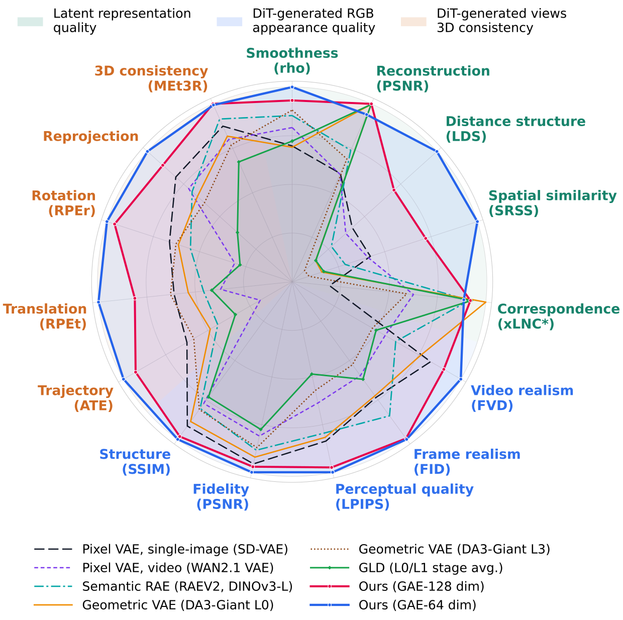
GAE compresses features from a frozen geometry model into one latent state that decodes to both RGB images and geometry. Under a shared generation protocol, its 64-channel version reduces FVD by 12.7% on RealEstate10K and 23.1% on DL3DV against the best competing latent. Independently recovered camera trajectories also improve. The controlled tests use nine-view clips; longer and text-conditioned examples come from a separately trained model. Project · Code.
1 Introduction
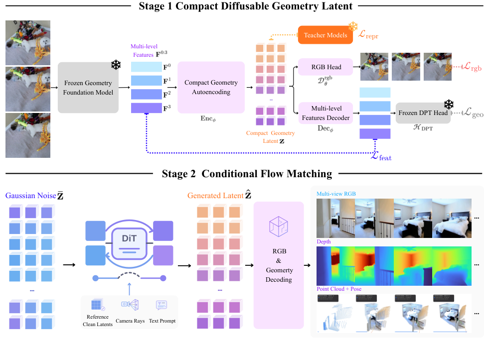
A video can look plausible while its scene geometry changes between views. GAE makes geometry part of the generated representation: it compresses all four DA3 feature levels, reconstructs them for the original frozen geometry head, and adds an RGB decoder. Semantic and spatial supervision organize the compact state for flow matching. This studies the choice of latent representation, with generator architecture and training held largely fixed. [18], [41], [12], [33].
2 Related Work
Generative representation spaces.
Pixel VAEs compress appearance; RAEs reuse pretrained semantic features. Reconstruction quality alone does not establish how easily a latent can be generated. GAE adds native geometry decoding while learning a compact representation. [29], [57], [33], [58].
Geometry-aware visual generation.
Earlier methods introduce geometry through explicit scenes, camera controls, joint output modalities, or additional training objectives. GAE instead generates a single state derived from a geometry foundation model. [25], [13], [7], [10], [1].
Geometry foundation models as generative states.
GLD generates a cascade of geometry features; latent Riemannian flow matching evolves four feature levels jointly. GAE learns a compact Euclidean bottleneck and reconstructs the hierarchy afterward, so one standard flow model can generate it. [12], [47].
3 Method
Training has two stages: learn a codec and RGB decoder around a frozen geometry backbone, then freeze the codec and train a conditional flow over its standardized posterior means. At sampling time, only requested output latents evolve; reference images, cameras, and text remain fixed conditions.
Equations 1–2
| (1) |
| (2) |
3.1 Geometry-native codec
Fusing all four DA3 levels retains complementary geometry cues while avoiding direct generation of the full high-dimensional hierarchy.
From a feature hierarchy to one state.
Normalize each feature level with fixed training-set channel statistics, reshape tokens to spatial grids, and concatenate channels. Shallow features retain detail and correspondence; deeper features supply complementary inputs expected by the geometry decoder.
Equation 3
| (3) |
Compact geometry codec.
A convolutional codec with spatial attention preserves the patch grid and compresses channels to 64 or 128, versus 3,072 for one raw DA3 level. Codec training samples a lightly KL-regularized posterior; generation uses its deterministic mean.
Equations 4–6
| (4) | ||||
| (5) | ||||
| (6) |
Joint RGB and geometry decoding.
The learned RGB head reads the bottleneck directly. A second decoder reconstructs all four feature levels for the frozen DPT geometry head, producing depth, rays, and point maps. Freezing that head requires retained information to remain readable through DA3’s original interface.
Equation 7
| (7) |
Codec objective.
Training combines feature reconstruction, weak KL regularization, RGB pixel/perceptual losses, geometry losses, and representation shaping. Geometry supervision consists of DA3 pseudo-targets from original features, rather than measured depth ground truth.
Equation 8
| (8) |
3.2 Organizing the latent for generation
Token-wise alignment with C-RADIO improves semantic neighborhoods and transport diagnostics, but damages pairwise spatial structure. Matching posterior-token similarities to DINOv2 restores that structure. The representation weight is 0.25 and the relational multiplier is 8. After training, discard the teachers and projector, freeze the codec, and standardize latent channels. [8], [26], [54].
| Diffusability (single-view) | Diffusability (multi-view) | Structure (single-view) | Structure (cross-view) | |||||||
| Representation objective | effrank | effrank | LNC@5 | LDS | SRSS | xLNC | ||||
| Raw geometry (DA3-GIANT L0) | 0.876 | 11.3 | 0.793 | 9.3 | 0.353 | 0.102 | 0.123 | 0.642 | ||
| Raw geometry (DA3-GIANT L3) | 0.769 | 11.5 | 0.539 | 9.0 | 0.054 | 0.054 | 0.070 | 0.380 | ||
| None | 0.820 | 130 | 58.0 | 0.630 | 580 | 20.0 | 0.310 | 0.240 | 0.300 | 0.590 |
| 0.700 | 170 | 53.0 | 0.570 | 450 | 26.0 | 0.490 | 0.020 | 0.030 | 0.580 | |
| 0.674 | 227 | 51.3 | 0.564 | 356 | 45.2 | 0.498 | 0.444 | 0.553 | 0.591 | |
Equations 9–12
| (9) | ||||
| (10) | ||||
| (11) |
| (12) |
3.3 Conditional flow matching and generation
Flow matching.
A transformer jointly predicts clean target-view latents along a linear data-to-noise path. Convert these predictions to velocity and minimize conditional flow-matching error; all views share a timestep. [33], [20].
Equation 13
| (13) |
Reference, camera, and text conditioning.
Reference features must be encoded using observed references alone, because joint encoding with unavailable target views would leak context. Prepend clean reference tokens at timestep zero, exclude them from the prediction head, and keep every output slot noisy. Metric Plücker rays modulate self-attention; text enters cross-attention. Condition dropout enables several generation modes. [52].
Training and inference.
Train the codec on single- and multi-view data, then train the frozen-codec flow with both text-to-image and view-conditioned batches. Sampling integrates Gaussian noise from time one to zero and decodes the resulting state into appearance and geometry.
4 Experiments
Experiments separate intrinsic latent properties, real-image reconstruction, and generation. Reconstruction fidelity alone is insufficient evidence for generation quality.
Experimental setup.
Seven controlled variants use pixel, semantic, raw geometry, or GAE latents with the same flow family, camera controls, training budget, and sampling. Evaluation uses held-out pools of 64 scenes from each dataset, nine 252 × 252 views, one reference, 50 Euler steps, and CFG scale 2. The higher-resolution final model is evaluated qualitatively. [61], [19].
Ranking convention.
Blue cells rank only controlled variants, with displayed ties resolved using unrounded values. Gray GLD and Gen3R rows are complete external pipelines and are excluded from that ranking.
4.1 Latent-space study
Raw DA3 levels have 3,072 channels but effective ranks near ten and severe covariance anisotropy. GAE improves conditioning and compresses to 64 or 128 channels while retaining useful geometry. It does not win every diagnostic: semantic RAEv2 has stronger semantic neighborhoods, and raw L0 has stronger cross-view retrieval. GAE-64 favors compactness and spatial structure; GAE-128 retains more cross-view information.
| Diffusability (single-view) | Diffusability (multi-view) | Structure (single-view) | Structure (cross-view) | ||||||||
| Latent | effrank | effrank | LNC@5 | LDS | SRSS | xLNC | |||||
| Pixel VAE, single-image (SD-VAE) | 0.888 | 3.7 | 3.0 | 0.765 | 4.1 | 3.1 | 0.051 | 0.262 | 0.324 | 0.124 | |
| Pixel VAE, video (WAN2.1 VAE) | 0.847 | 127 | 5.3 | 0.609 | 160 | 4.3 | 0.084 | 0.234 | 0.313 | 0.402 | |
| Semantic RAE (RAEV2) | 0.711 | 289.3 | 0.640 | 93.3 | 0.932 | 0.171 | 0.220 | 0.587 | |||
| Raw geometry (DA3-GIANT L0) | 0.876 | 11.3 | 0.793 | 9.3 | 0.353 | 0.102 | 0.123 | 0.642 | |||
| Raw geometry (DA3-GIANT L3) | 0.769 | 11.5 | 0.539 | 9.0 | 0.054 | 0.054 | 0.070 | 0.380 | |||
| GLD (L0/L1 stage avg.) | – | 0.854 | 34.8 | 0.742 | 22.7 | 0.274 | 0.103 | 0.131 | 0.594 | ||
| Ours (GAE-128) | 0.674 | 227 | 51.3 | 0.564 | 356 | 45.2 | 0.498 | 0.444 | 0.553 | 0.591 | |
| Ours (GAE-64) | 0.634 | 53.1 | 37.0 | 0.519 | 117 | 33.2 | 0.488 | 0.631 | 0.767 | 0.569 | |
4.2 Codec reconstruction quality
4.2.1 RGB reconstruction
GAE-128 matches or slightly exceeds raw L0 RGB reconstruction with 24 times fewer channels: multi-view PSNR is 34.78 versus 34.70, and rFVD is 4.3 versus 4.4. GAE-64 loses some reconstruction fidelity. Single-view evaluation uses ImageNet; multi-view results average five datasets.
| Single-view | Multi-view | |||||
| Latent | PSNR | LPIPS | rFID | PSNR | LPIPS | rFVD |
| Pixel VAE, single-image (SD-VAE) | 18.49 | 0.140 | 10.1 | 19.97 | 0.121 | 37.7 |
| Pixel VAE, video (WAN2.1 VAE) | 18.34 | 0.125 | 8.9 | 19.83 | 0.163 | 46.7 |
| Semantic RAE (RAEV2) | 22.08 | 0.134 | 8.8 | 24.73 | 0.094 | 32.1 |
| Raw geometry (DA3-GIANT L0) | 28.64 | 0.038 | 5.5 | 34.70 | 0.014 | 4.4 |
| Raw geometry (DA3-GIANT L3) | 19.90 | 0.219 | 25.3 | 23.98 | 0.122 | 76.2 |
| Ours (GAE-128) | 28.76 | 0.036 | 5.4 | 34.78 | 0.014 | 4.3 |
| Ours (GAE-64) | 27.30 | 0.061 | 7.1 | 32.37 | 0.040 | 9.1 |
4.2.2 Geometry reconstruction
Both GAE widths improve depth, point-map, and pose reconstruction over the raw-L0 baseline. Depth and point references come from Pi3 estimates on real frames; poses use dataset cameras. External Gen3R is slightly better on some depth measures. Pixel and semantic codecs lack the required native geometry decoder. [45].
| RealEstate10K (Pi3 ref) | DL3DV (Pi3 ref) | |||||||||||
|---|---|---|---|---|---|---|---|---|---|---|---|---|
| Method | AbsRel | Cham. | PMap | ATE | RPEr | AbsRel | Cham. | PMap | ATE | RPEr | ||
| Pi3 on real (ref) | — | — | — | — | 0.009 | 0.17 | — | — | — | — | 0.011 | 0.26 |
| Gen3R | 0.085 | 0.906 | 0.430 | 0.829 | 0.038 | 0.63 | 0.114 | 0.862 | 0.237 | 0.542 | 0.022 | 0.72 |
| GLD | 0.271 | 0.694 | 0.857 | 1.580 | 0.039 | 1.23 | 0.303 | 0.608 | 0.462 | 1.083 | 0.026 | 1.14 |
| Raw geometry (DA3-GIANT L0) | 0.178 | 0.759 | 0.635 | 1.160 | 0.068 | 1.33 | 0.234 | 0.639 | 0.575 | 1.130 | 0.057 | 1.09 |
| Ours (GAE-128) | 0.090 | 0.905 | 0.400 | 0.700 | 0.006 | 0.19 | 0.125 | 0.862 | 0.145 | 0.433 | 0.008 | 0.25 |
| Ours (GAE-64) | 0.090 | 0.905 | 0.386 | 0.691 | 0.007 | 0.20 | 0.125 | 0.861 | 0.145 | 0.433 | 0.008 | 0.27 |
4.3 Flow-matching generation quality
The same controlled flow recipe tests how latent choice affects generated RGB and geometry.
4.3.1 RGB generation
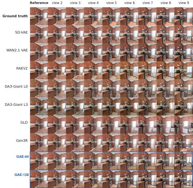
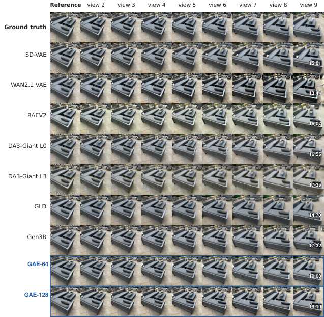
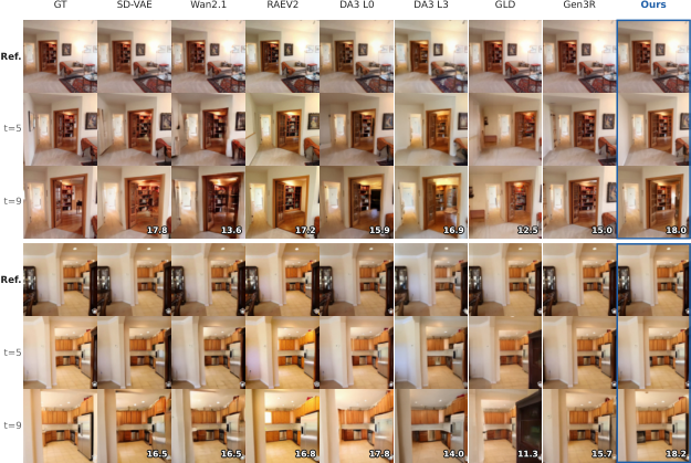
GAE-64 reduces FVD from the strongest non-GAE controlled baseline’s 258.6 to 225.7 on RealEstate10K and from 373.2 to 287.0 on DL3DV. It leads the paired image metrics; GAE-128 has the best RealEstate10K FID. Scene examples illustrate preserved appearance as the camera moves.
| RealEstate10K | DL3DV | |||||||||
|---|---|---|---|---|---|---|---|---|---|---|
| Latent | FVD | FID | LPIPS | PSNR | SSIM | FVD | FID | LPIPS | PSNR | SSIM |
| Pixel VAE, single-image (SD-VAE) | 258.6 | 36.4 | 0.171 | 19.32 | 0.666 | 373.2 | 57.1 | 0.232 | 17.05 | 0.495 |
| Pixel VAE, video (WAN2.1 VAE) | 362.9 | 41.0 | 0.219 | 16.52 | 0.575 | 596.7 | 77.3 | 0.313 | 14.31 | 0.407 |
| Semantic RAE (RAEV2) | 379.4 | 31.4 | 0.191 | 17.60 | 0.585 | 453.4 | 49.2 | 0.231 | 16.01 | 0.434 |
| Raw geometry (DA3-GIANT L0) | 298.6 | 35.5 | 0.177 | 18.31 | 0.643 | 376.5 | 60.2 | 0.235 | 16.68 | 0.481 |
| Raw geometry (DA3-GIANT L3) | 488.9 | 50.0 | 0.273 | 16.82 | 0.579 | 584.8 | 80.6 | 0.314 | 16.22 | 0.447 |
| Ours (GAE-128) | 233.4 | 25.6 | 0.146 | 19.54 | 0.701 | 345.2 | 44.2 | 0.200 | 17.39 | 0.541 |
| Ours (GAE-64) | 225.7 | 27.1 | 0.143 | 20.02 | 0.711 | 287.0 | 41.3 | 0.194 | 18.00 | 0.553 |
| GLD | 445.1 | 44.0 | 0.337 | 14.91 | 0.518 | 587.4 | 66.4 | 0.356 | 14.51 | 0.406 |
| Gen3R | 269.7 | 25.7 | 0.196 | 17.79 | 0.621 | 580.5 | 48.3 | 0.270 | 15.62 | 0.440 |
4.3.2 3D consistency
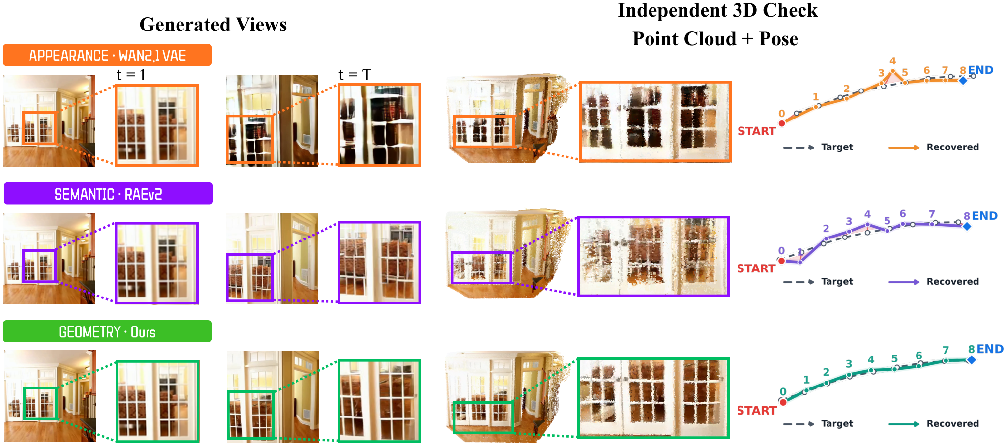
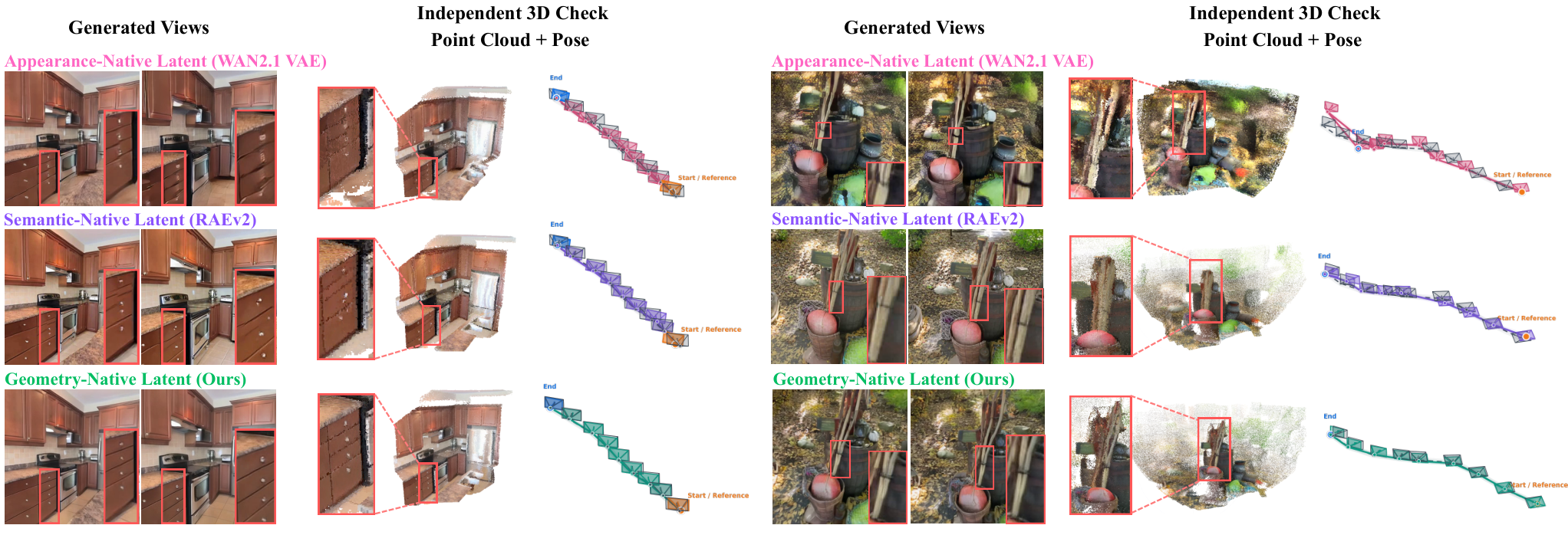
Independent VGGT reconstruction gives GAE-64 ATE of 0.0034 versus the best competing controlled latent’s 0.0072 on RealEstate10K, and 0.0056 versus 0.0073 on DL3DV. These correspond to 52.8% and 23.3% reductions after Sim(3) alignment. The two GAE widths also lead controlled MEt3R scores. DA3 results are a backbone-overlap cross-check; external Gen3R has a better RealEstate10K MEt3R score. [41], [2].
| VGGT (independent) | DA3-GIANT (cross-check) | ||||||||
| Latent | ATE | RPEt | RPEr | Reproj. | ATE | RPEt | RPEr | Reproj. | MEt3R |
| RealEstate10K | |||||||||
| Pixel VAE, single-image (SD-VAE) | 0.0072 | 0.0182 | 0.648 | 0.0093 | 0.0046 | 0.0191 | 0.338 | 0.0018 | 0.1385 |
| Pixel VAE, video (WAN2.1 VAE) | 0.0225 | 0.0252 | 0.746 | 0.0105 | 0.0135 | 0.0176 | 0.751 | 0.0019 | 0.1441 |
| Semantic RAE (RAEV2) | 0.0085 | 0.0233 | 0.420 | 0.0104 | 0.0066 | 0.0219 | 0.507 | 0.0019 | 0.1263 |
| Raw geometry (DA3-GIANT L0) | 0.0085 | 0.0202 | 0.435 | 0.0096 | 0.0047 | 0.0167 | 0.358 | 0.0020 | 0.1420 |
| Raw geometry (DA3-GIANT L3) | 0.0112 | 0.0211 | 0.516 | 0.0124 | 0.0036 | 0.0148 | 0.355 | 0.0019 | 0.1575 |
| Ours (GAE-128) | 0.0041 | 0.0173 | 0.332 | 0.0075 | 0.0026 | 0.0143 | 0.304 | 0.0017 | 0.1213 |
| Ours (GAE-64) | 0.0034 | 0.0060 | 0.380 | 0.0068 | 0.0026 | 0.0141 | 0.225 | 0.0013 | 0.1208 |
| GLD | 0.0124 | 0.0258 | 0.886 | 0.0133 | 0.0088 | 0.0221 | 0.950 | 0.0038 | 0.1660 |
| Gen3R | 0.0090 | 0.0213 | 0.423 | 0.0072 | 0.0063 | 0.0211 | 0.387 | 0.0014 | 0.1157 |
| DL3DV | |||||||||
| Pixel VAE, single-image (SD-VAE) | 0.0073 | 0.0098 | 0.432 | 0.0108 | 0.0055 | 0.0076 | 0.358 | 0.0024 | 0.1542 |
| Pixel VAE, video (WAN2.1 VAE) | 0.0243 | 0.0288 | 1.419 | 0.0258 | 0.0206 | 0.0251 | 1.016 | 0.0019 | 0.1777 |
| Semantic RAE (RAEV2) | 0.0104 | 0.0143 | 0.638 | 0.0130 | 0.0088 | 0.0113 | 0.585 | 0.0031 | 0.1549 |
| Raw geometry (DA3-GIANT L0) | 0.0110 | 0.0136 | 0.634 | 0.0129 | 0.0079 | 0.0102 | 0.482 | 0.0042 | 0.1721 |
| Raw geometry (DA3-GIANT L3) | 0.0097 | 0.0120 | 0.603 | 0.0151 | 0.0052 | 0.0073 | 0.380 | 0.0039 | 0.1754 |
| Ours (GAE-128) | 0.0056 | 0.0072 | 0.294 | 0.0080 | 0.0043 | 0.0053 | 0.260 | 0.0029 | 0.1347 |
| Ours (GAE-64) | 0.0056 | 0.0066 | 0.293 | 0.0077 | 0.0038 | 0.0053 | 0.254 | 0.0028 | 0.1370 |
| GLD | 0.0136 | 0.0164 | 1.242 | 0.0241 | 0.0104 | 0.0136 | 1.048 | 0.0087 | 0.2183 |
| Gen3R | 0.0096 | 0.0133 | 0.678 | 0.0143 | 0.0096 | 0.0131 | 0.608 | 0.0065 | 0.1662 |
4.3.3 Geometry generation
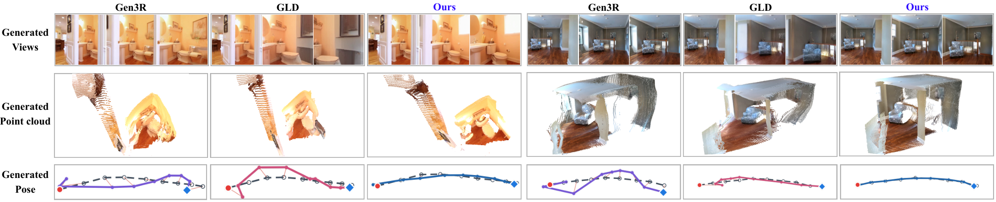
Decoded depth and point maps are compared with Pi3 on real target frames, while decoded poses are compared with dataset cameras. GAE-64 leads controlled geometry-native variants on all six DL3DV metrics; GAE-128 has better RealEstate10K point-cloud and point-map errors. These reference estimates are independent of DA3, but are still model-derived geometry.
| RealEstate10K (Pi3 ref) | DL3DV (Pi3 ref) | |||||||||||
|---|---|---|---|---|---|---|---|---|---|---|---|---|
| Method | AbsRel | Cham. | PMap | ATE | RPEr | AbsRel | Cham. | PMap | ATE | RPEr | ||
| Pi3 on real (ref) | — | — | — | — | 0.009 | 0.17 | — | — | — | — | 0.011 | 0.26 |
| Gen3R | 0.164 | 0.807 | 0.727 | 1.428 | 0.046 | 0.69 | 0.232 | 0.688 | 0.587 | 1.180 | 0.031 | 0.91 |
| GLD | 0.271 | 0.694 | 0.858 | 1.580 | 0.039 | 1.23 | 0.323 | 0.594 | 0.462 | 1.097 | 0.028 | 1.19 |
| Raw geometry (DA3-GIANT L0) | 0.157 | 0.822 | 0.540 | 1.058 | 0.019 | 0.35 | 0.245 | 0.715 | 0.330 | 0.815 | 0.019 | 0.48 |
| Ours (GAE-128) | 0.139 | 0.849 | 0.432 | 0.813 | 0.013 | 0.37 | 0.225 | 0.750 | 0.325 | 0.832 | 0.016 | 0.40 |
| Ours (GAE-64) | 0.134 | 0.857 | 0.501 | 0.924 | 0.010 | 0.33 | 0.204 | 0.765 | 0.262 | 0.698 | 0.014 | 0.36 |
4.3.4 Additional qualitative capabilities
Long-rollout showcase.
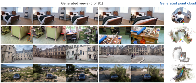
A separate model jointly samples 81 views at 672 × 378 from one reference. Its point cloud concatenates decoded, unprojected depth maps using cameras recovered from decoded rays, without cross-view fusion or test-time optimization. These selected examples demonstrate longer generation, not a controlled long-horizon benchmark.
Text-conditioned generation.
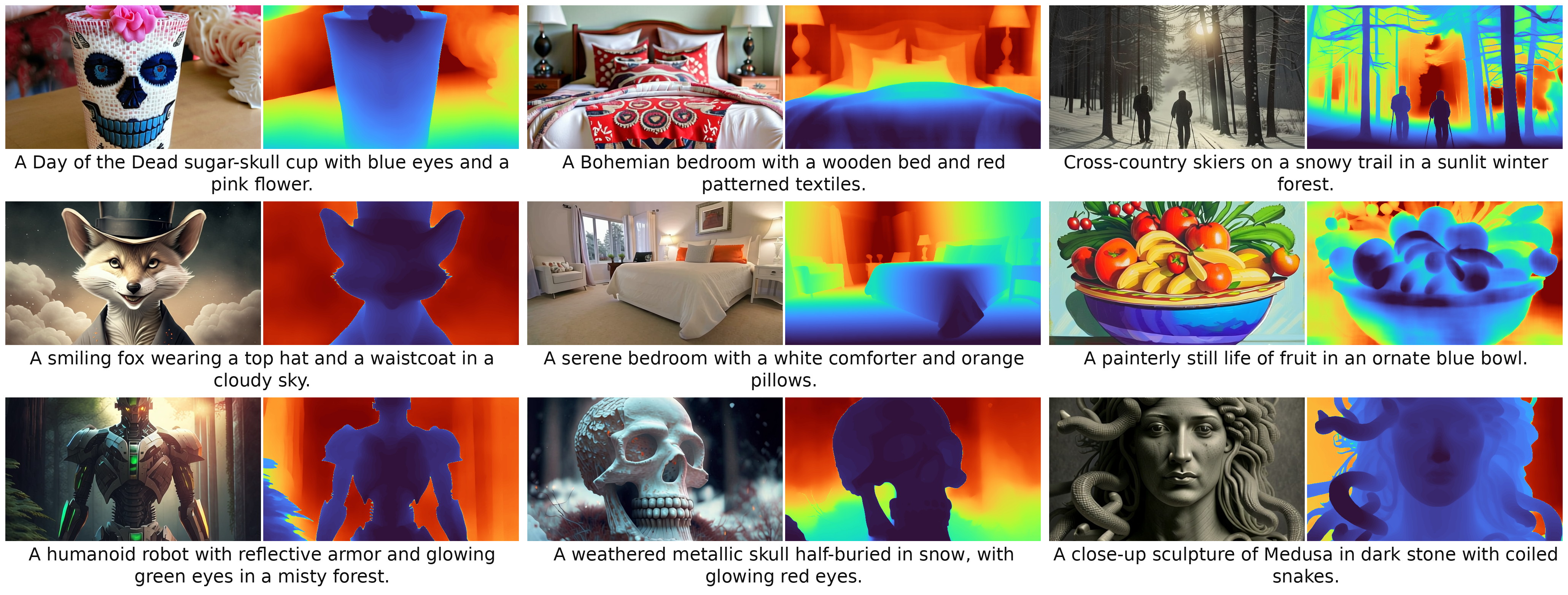
The same final checkpoint generates RGB and depth from text. Selected prompts demonstrate capability; no standalone text-to-image benchmark is reported.
4.4 Ablation studies
Representation shaping improves GIANT-128 generation, while the larger backbone improves appearance and pose but slightly worsens MEt3R against LARGE-128. Clean reference tokens lower the reference–target point-cloud gap from 0.1016 to 0.0318. Metric camera scale lowers scale-sensitive ATE from 0.0346 to 0.0093. Text-to-image co-training lowers FVD from 472.9 to 225.7.
| Setting | FVD | PSNR | MEt3R | Diag. |
|---|---|---|---|---|
| Codec design (Diag. VGGT ATE) | ||||
| LARGE-128, with | 270.5 | 19.12 | 0.1192 | 0.0048 |
| GIANT-128, no | 266.4 | 19.19 | 0.1226 | 0.0044 |
| GIANT-128, with | 233.4 | 19.54 | 0.1213 | 0.0041 |
| Reference conditioning (Diag. Ref–tgt PC gap) | ||||
| Reference latent in ODE state | 257.1 | 18.91 | 0.1217 | 0.1016 |
| Clean conditioning token | 225.7 | 20.02 | 0.1208 | 0.0318 |
| Pose scale (Diag. SE(3) ATE, no Sim(3)) | ||||
| Per-scene normalized pose | 350.7 | 16.28 | 0.1290 | 0.0346 |
| Metric pose | 225.7 | 20.02 | 0.1208 | 0.0093 |
| Text-to-image co-training (Diag. LPIPS) | ||||
| Without T2I co-training | 472.9 | 16.77 | 0.1262 | 0.199 |
| With T2I co-training | 225.7 | 20.02 | 0.1208 | 0.143 |
5 Conclusion
A compact state that preserves geometry can improve controlled view generation. The evidence is limited to the reported datasets, estimator-based geometry checks, and training recipes; the paper provides no repeated-run uncertainty or quantitative long-horizon evaluation. The larger model also uses internally curated training data, so its selected examples do not isolate the latent’s contribution.
Appendix A Implementation and evaluation details
A.1 Geometry-native codec details
The frozen DA3-GIANT encoder and geometry head surround the learned codec. Training reconstructs its four feature levels, RGB, and geometry pseudo-targets. C-RADIO, DINOv2, and their projector are needed only while learning the codec.
A.2 Flow-matching parameterization
Predict a clean latent, then divide the noisy-to-clean difference by max(t, 0.05) to obtain velocity. Controlled models use a DDT-style encoder–decoder transformer with 28 width-768 encoder blocks and six width-2048 decoder blocks. Cross-view attention processes 1 × 1 latent tokens; temporal models add frame-axis rotary embeddings.
Equations 14–16
| (14) |
| (15) |
| (16) |
A.3 Inference-aligned multimodal conditioning
Only requested outputs are numerical flow states. References provide clean evidence, cameras provide spatial control, and text provides semantic context.
Reference tokens.
Encode the observed reference set once, prepend its standardized latents at timestep zero, and keep these tokens outside the output head and solver. Outputs at reference-camera poses are still generated normally; reference tokens are never repeatedly clamped into the noisy state.
Equation 17
| (17) |
Camera rays.
Represent each camera ray by its direction, normalized moment, and logarithmic moment magnitude. The last component preserves metric translation scale when metric camera data are available. Evaluate rays on the transformer token grid and use them to modulate attention queries and keys. [52].
Equation 18
| (18) |
Text.
Frozen language-model features condition cross-attention. Independent text, camera, and reference dropout supports different condition combinations and supplies branches for classifier-free guidance. [9].
A.4 Two-stage training and sampling
Freeze all codec modules before training the flow. Every sampling run starts with Gaussian output latents, uses fixed clean reference conditions, and finishes by denormalizing and decoding.
Controlled latent comparison.
Controlled models mix RealEstate10K and DL3DV equally, with nine-view training clips and one to four prefix references. The shared flow has approximately 0.93 billion parameters, excluding frozen modules, and trains on eight GPUs with BF16, AdamW, and EMA. Learning rate warms up for 2,000 steps to 10⁻⁴ and decays toward 10⁻⁶ over 100,000 steps. Qwen3-0.6B supplies text features; one text-to-image batch follows every three multi-view updates. Pixel and semantic outputs are resized from 256 to 252 pixels for evaluation. [50].
Final model.
The separate final model trains on 81-view clips at 672 × 378 using 80 GPUs and a 60,000-step schedule. Data include six named public collections plus internally curated sets. The approximately 0.93-billion-parameter count covers only the trainable flow. One text-to-image batch follows every four multi-view updates; text, camera, and reference dropout rates are 0.10, 0.20, and 0.20. Showcases use 50 Euler steps and CFG 2, retaining camera control in the unconditional branch. [51], [11], [40], [62].
A.5 Controlled evaluation protocol
Distributional metrics use frames and clips; paired metrics compare requested views with real targets. Camera metrics use Sim(3)-aligned recovered trajectories. Reprojection retains the highest-confidence half of points; MEt3R averages visibility-masked feature disagreement across view pairs. Native depth is median-scale aligned per view, while point clouds use trajectory alignment. Consequently, the standard geometry results do not establish absolute metric-scale accuracy; the scale ablation addresses that separately.
Appendix B Latent-space diagnostic definitions
The diagnostics describe transport ambiguity, covariance conditioning, semantic organization, spatial structure, and cross-view correspondence. They are complementary proxies, not interchangeable measures of generation quality.
Evaluation data and preprocessing.
Single-view tests use ImageNet-S classes and foreground masks; multi-view tests group frames by scene. Spatial thresholds use shared image coordinates, and cosine comparisons normalize tokens. Reported latents receive no diagnostic-only PCA removal or centering. [5].
Within-group velocity fraction ρ (lower is better).
The variance ratio divides within-class or within-scene covariance trace by total covariance trace. Lower values indicate more compact groups relative to overall variation, interpreted here as less ambiguous transport.
Equation 19
| (19) |
Condition number κ and effective rank (lower/higher is better).
Condition number measures the largest-to-smallest covariance eigenvalue ratio. Effective rank is the squared eigenvalue sum divided by the sum of squared eigenvalues. Together they distinguish nominal channel count from the number and balance of active directions.
Equation 20
| (20) |
Latent neighbor consistency LNC@5 (higher is better).
LNC@5 foreground-pools each image latent and measures how often its five nearest descriptors share its class. It evaluates local semantic organization, not patch-level geometry.
Latent distance structure LDS (higher is better).
LDS subtracts average similarity of distant token pairs from that of nearby pairs, using nearby (approximately 24 pixels) and distant (approximately 96 pixels) neighborhoods. A higher score means similarity better reflects spatial proximity.
Equation 21
| (21) |
Spatial relative similarity score SRSS (higher is better).
SRSS compares a foreground token’s similarity to nearby foreground positives against distant background negatives. A higher score indicates spatially coherent foreground regions that remain distinct from background.
Equation 22
| (22) |
Cross-view latent neighbor consistency xLNC ∗ (higher is better).
UFM-Refine provides cross-view correspondences. Retrieve each matched token’s nearest latent neighbor in the other view, count neighborhood matches, and normalize accuracy against chance. xLNC* equals zero at chance and one for perfect retrieval; evaluation requires sufficient view overlap. [56].
Equation 23
| (23) |
Appendix C Additional qualitative comparisons
C.1 Independent 3D check
Additional scenes compare generated RGB, point clouds, and camera paths under identical controls. VGGT reconstructs all outputs independently of the generating latent backbone.
C.2 RGB comparisons
The appendix displays all nine views for one RealEstate10K scene and one DL3DV scene. Each shown PSNR covers that scene’s eight generated target views, not the complete dataset.