At a glance
HappyWorld-Bench tests whether generated environments remain coherent when explored, acted on, and modified. Its independent video, spatial, and embodied tracks contain 1,138 prompts, 300 scenes, and 254 task instances or intervention groups. The study compares 14 interactive video models, nine spatial systems, and eight embodied video generators; five additional conventional video generators enter the W1 comparison. Strong images do not consistently imply dependable state, contact, or intervention responses. The W1–W6 hierarchy is a proposed organizing framework: reported tests cover video W1–W4, spatial W1–W5, and embodied W2–W4, with no W6 score.

1 Introduction
A useful world model must predict changes caused by actions while preserving geometry, identity, and prior state. Existing evaluations often isolate appearance, memory, interaction, or geometry. This benchmark combines a shared capability vocabulary with separate tests appropriate to video generation, explicit spatial scenes, and robot-centric visual prediction. [34] [53] [91]
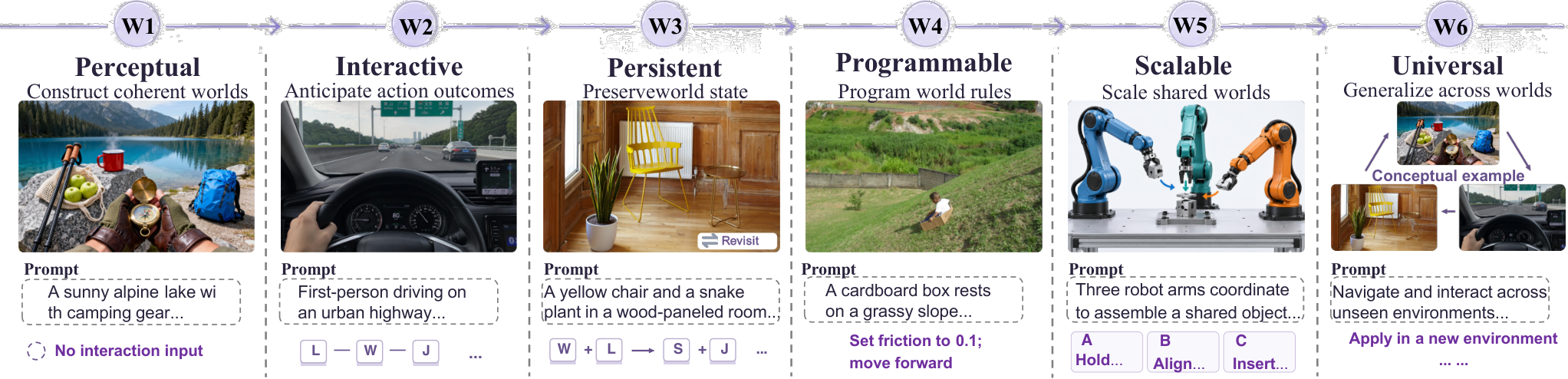
Contributions.
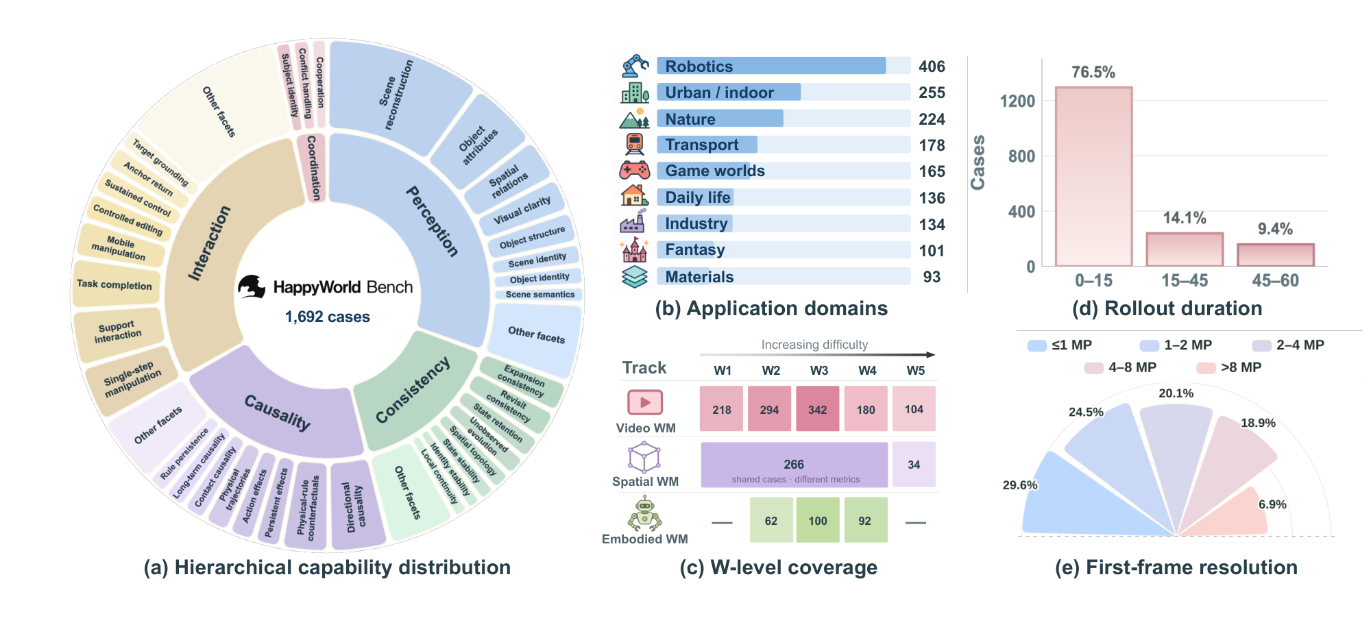
The hierarchy progresses from perceptual construction through interaction, persistence, intervention, shared-world scalability, and universal modeling. The three tracks instantiate different parts of this aspiration and retain separate human-preference Elo ratings. Their 1,692 track-specific instances span varied domains, image sizes, and rollout lengths; these are not 1,692 interchangeable tests. Human preference complements behavioral metrics rather than replacing them.
| Level | Scope Defintion |
| W1: Perceptual World | Construct a coherent world representation from visual or multimodal conditions, with correct semantics, spatial structure, and short-term temporal continuity. |
| W2: Interactive World | Simulate action-conditioned state transitions, predicting how agents, objects, and environments evolve in response to interaction while preserving local geometric, physical, and causal consistency. |
| W3: Persistent World | Maintain global spatial structure, object identity, and accumulated world states over long-horizon interaction, viewpoint changes, occlusion, and revisitation. |
| W4: Programmable World | Support explicit interventions on objects, events, behaviors, or world rules, with intended changes propagated causally while unaffected content remains consistent. |
| W5: Scalable World | Generate infinitely extensible world states shared by multiple embodied or virtual agents, supporting agent communication, synchronization, cooperation, and conflict handling under partial observability. |
| W6: Universal World | Integrate generation, simulation, persistent state modeling, interaction, and planning into a unified system that fully replicates the real world and generalizes across environments, tasks, modalities, and embodiments. |
2 Related Work
Prior work supplies the model families and evaluation methods compared below.
2.1 World Model
The three model families differ in what they represent and how users intervene.
Video world models
Interactive video systems have added keyboard, camera, language, and history conditioning to generative rollouts. Longer context and memory improve exploration, but the benchmark asks whether these interfaces preserve state and obey interventions in their evaluated configurations. [14] [92] [39]
Spatial world models
Spatial methods build renderable meshes or Gaussian scenes from panoramas, generated videos, or explicit programs. Their outputs support tests of geometry, navigation, object visibility, editing, and expansion. The evaluated GPT-6-Astra baseline constructs Blender meshes, a substantially different representation from image-driven reconstruction. [111] [110] [101]
Embodied world models
Embodied world models range from latent predictive states to action-conditioned video and joint video/action systems. This track selects visual generation as the common interface; its findings concern generated robot-centric observations rather than policy execution on physical robots. [36] [67] [99]
2.2 World Model Benchmarks
Existing benchmarks emphasize complementary aspects of quality, interaction, persistence, or downstream utility.
Video world model benchmarks
Video benchmarks have expanded from visual quality toward camera following, memory, physical plausibility, interventions, and closed-loop goals. HappyWorld-Bench organizes these concerns into capability-specific tests while preserving distinct metrics for appearance and behavioral correctness. [43] [62] [121]
Spatial world model benchmarks
Spatial evaluation combines asset quality, scene semantics, support, navigation, and exploration. Here rendered views, exported geometry, and matched before/after operations jointly test construction, usable space, persistence, editing, and growth. [29] [89] [28]
Embodied world model benchmarks
Embodied evaluations can assess generated appearance, action fidelity, or downstream policy utility. This work targets the first two: a reference image plus an action prompt produces a video, without a robot, simulator-driven policy, or action decoder in the evaluation loop. [112] [54] [76]
3 Video World Model Track
Video tests examine natural evolution, control response, revisitation, and language-based intervention.
3.1 Data Construction
Human-reviewed cases pair a reference image and descriptions with capability-specific controls.
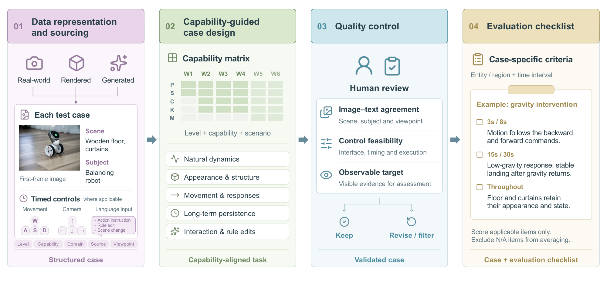
Data representation and sourcing.
Each record specifies its initial image, scene and subject descriptions, viewpoint, and timed controls where applicable. W1 has no external action; W2–W3 prescribe directions and intervals rather than exact poses. W4 adds natural-language actions or rule changes. The schema permits subject-specific controls for higher levels, without establishing that those levels are evaluated here.
Capability-guided case design.
Cases probe uncontrolled natural motion, appearance under viewpoint changes, timed movement and environmental response, landmark revisits, and interventions whose effects should persist while unrelated content stays stable.
Quality control.
Reviewers check image–description agreement, executable timing and controls, and observable evaluation targets. Ambiguous, infeasible, or visually unassessable cases are removed.
Dataset Statistics
The 1,138 cases comprise 218 W1, 294 W2, 342 W3, 180 W4, and 104 W5 cases. A separate categorization assigns 74 facets across perception, consistency, causality, control, and multi-subject coordination. W5 is represented in the collection but has no reported video leaderboard in this paper.
3.2 Evaluation Metrics
Perception uses image quality, learned preference, imaging stability, motion amount, and instruction checks. Consistency combines masked appearance features, depth/pose reprojection, and state judgments. Causality uses visible physical and event checklists. W2–W3 control scores assess translation direction and action completion; W4 instead checks the intervention process and resulting state. These learned evaluators and visibility-based judgments are proxies with metric-specific applicability. [49] [64]
3.3 Experimental Results
Results separate human preference from the capability scores and their component metrics.
Experimental setup.
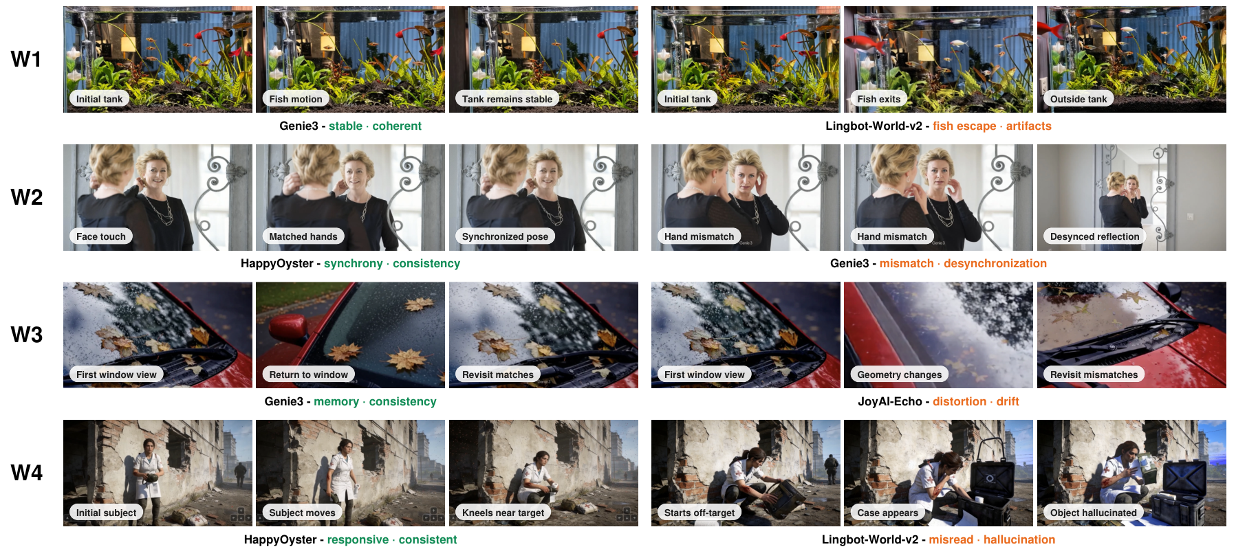
HappyOyster leads video Arena Elo at 1263, followed by Genie 3 at 1206. Genie 3 leads W1 at 82.8 versus 82.4; HappyOyster leads W2 and W3 at 78.0 and 76.8. Only HappyOyster and LingBot-World-v2 enter W4, scoring 66.7 and 59.3. The tables reveal distinct weaknesses in geometry, persistent state, and intervention effects despite attractive frames. W2 and W3 use different case pools, so differences are not a controlled duration effect. W4 judges later behavior against the edited rule, including preservation of unaffected content. Appendix A documents substantial input adaptations and unsupported controls. [74] [5] [117]
| Model | Arena Elo | W1 | W2 | W3 | W4 |
| HappyOyster | 1263 | 82.4 | 78.0 | 76.8 | 66.7 |
| Genie 3 | 1206 | 82.8 | 74.0 | 75.0 | - |
| JoyAI-Echo | 1147 | 78.2 | 74.5 | 74.1 | - |
| Alaya-EVOKE | 1132 | 79.2 | 73.9 | 74.6 | - |
| Lingbot-World-v2 | 1115 | 81.9 | 72.6 | 71.0 | 59.3 |
| Cosmos3 | 1092 | 81.3 | 70.2 | 64.8 | - |
| Yume-1.5 | 1063 | 79.6 | 70.2 | 67.7 | - |
| Lyra 2.0 | 1059 | 81.0 | 73.5 | 71.6 | - |
| DreamX-World | 1041 | 80.3 | 72.7 | 72.4 | - |
| MatrixGame-3.0 | 943 | 78.8 | 64.6 | 66.1 | - |
| SANA-WM | 917 | 78.0 | 64.0 | 62.4 | - |
| MatrixGame-2.0 | 856 | 63.4 | 61.1 | 59.6 | - |
| ABot-World | 843 | 69.0 | 64.6 | 60.4 | - |
| Open-Oasis | 324 | 53.1 | 43.3 | 39.4 | - |
| Perception | Consistency | |||||||||
| Model | VQ | HPS | IS | Dyn | IF | BC | GC | TC | SC | SuC |
| ABot-World | 60.89 | 53.94 | 59.86 | 10.58 | 88.78 | 92.28 | 97.92 | 70.11 | 63.94 | 92.13 |
| Alaya-EVOKE | 66.41 | 68.43 | 82.98 | 51.77 | 95.03 | 94.50 | 98.42 | 74.62 | 64.86 | 94.90 |
| DreamX-World | 67.40 | 70.20 | 75.25 | 99.63 | 93.59 | 93.59 | 96.95 | 46.26 | 66.88 | 93.74 |
| Genie 3 | 70.46 | 70.79 | 83.27 | 85.14 | 90.16 | 94.86 | 97.91 | 60.85 | 82.30 | 92.50 |
| HappyHorse 1.1 | 70.51 | 75.74 | 84.32 | 62.93 | 96.06 | 96.67 | 98.05 | 54.41 | 71.47 | 95.28 |
| HappyOyster | 68.32 | 71.85 | 89.76 | 60.01 | 95.83 | 97.43 | 98.43 | 69.01 | 77.80 | 95.44 |
| JoyAI-Echo | 66.06 | 64.31 | 76.49 | 70.13 | 90.58 | 94.26 | 98.11 | 60.11 | 68.90 | 93.30 |
| Kling 3.0 | 69.20 | 73.24 | 85.35 | 52.29 | 95.89 | 97.18 | 98.23 | 63.16 | 71.10 | 96.10 |
| Lingbot-World-v2 | 68.32 | 73.55 | 85.24 | 52.20 | 95.20 | 97.00 | 98.76 | 75.46 | 76.97 | 96.47 |
| Lyra 2.0 | 68.06 | 69.38 | 86.26 | 4.50 | 95.83 | 97.98 | 99.44 | 94.19 | 96.42 | 98.18 |
| MatrixGame-2.0 | 63.63 | 46.34 | 75.22 | 0.00 | 82.65 | 90.25 | 98.07 | 56.99 | 27.98 | 92.38 |
| MatrixGame-3.0 | 68.75 | 71.05 | 75.20 | 13.18 | 92.02 | 95.55 | 99.35 | 82.49 | 95.41 | 94.87 |
| MiniMax-H3 | 68.66 | 69.90 | 88.49 | 46.16 | 96.45 | 97.27 | 98.48 | 71.36 | 83.39 | 96.00 |
| Cosmos3 | 67.77 | 69.62 | 94.43 | 11.65 | 95.02 | 97.26 | 99.35 | 92.12 | 89.08 | 97.05 |
| Open-Oasis | 47.88 | 14.92 | 45.83 | 1.90 | 81.55 | 83.84 | 97.06 | 44.85 | 22.29 | 90.79 |
| SANA-WM | 66.74 | 59.07 | 84.88 | 65.79 | 91.10 | 95.42 | 98.37 | 61.35 | 64.13 | 93.32 |
| Seedance2.5 | 67.42 | 73.10 | 90.28 | 36.82 | 95.06 | 97.53 | 98.57 | 76.76 | 83.79 | 96.79 |
| Wan 3.0 | 69.60 | 77.97 | 84.51 | 62.39 | 95.81 | 96.63 | 97.88 | 58.78 | 74.22 | 94.69 |
| Yume-1.5 | 69.35 | 67.61 | 66.52 | 86.88 | 93.92 | 94.62 | 97.42 | 61.02 | 64.50 | 93.75 |
| Perception | Consistency | Causality | Interaction | ||||||||||||
| Model | VQ | HPS | IS | Dyn | IF | BC | GC | TC | SC | SuC | PC | CC | IP | TA | AE |
| ABot-World | 59.33 | 48.09 | 49.50 | 48.32 | 88.46 | 87.68 | 90.93 | 51.45 | 40.61 | 87.52 | 56.45 | 53.54 | 86.74 | 59.38 | 65.91 |
| Alaya-EVOKE | 66.61 | 64.87 | 68.81 | 88.84 | 91.81 | 89.77 | 92.62 | 41.42 | 57.89 | 88.89 | 73.68 | 62.80 | 96.32 | 70.61 | 64.83 |
| DreamX-World | 64.64 | 62.52 | 70.15 | 99.82 | 91.52 | 90.30 | 89.88 | 32.98 | 52.15 | 89.43 | 69.30 | 60.20 | 91.68 | 72.09 | 64.84 |
| Genie 3 | 68.55 | 66.84 | 67.76 | 88.87 | 91.71 | 90.48 | 93.93 | 47.32 | 67.99 | 87.60 | 78.64 | 59.80 | 97.07 | 67.89 | 58.62 |
| HappyOyster | 67.25 | 67.82 | 73.98 | 81.25 | 94.14 | 93.79 | 91.36 | 35.94 | 65.60 | 90.35 | 84.90 | 77.51 | 95.96 | 67.31 | 80.20 |
| JoyAI-Echo | 65.84 | 59.92 | 67.02 | 87.73 | 90.87 | 90.33 | 90.15 | 38.15 | 62.04 | 87.80 | 75.76 | 67.33 | 94.03 | 72.58 | 69.53 |
| Lingbot-World-v2 | 65.98 | 64.21 | 65.12 | 81.68 | 91.66 | 90.68 | 88.90 | 40.77 | 52.18 | 87.71 | 68.92 | 60.48 | 94.38 | 73.48 | 66.61 |
| Lyra 2.0 | 66.51 | 59.04 | 69.98 | 56.05 | 92.89 | 91.60 | 91.71 | 52.35 | 71.77 | 90.66 | 67.90 | 59.46 | 93.53 | 76.28 | 67.28 |
| MatrixGame-2.0 | 63.22 | 43.90 | 63.90 | 45.29 | 83.54 | 87.78 | 91.85 | 43.57 | 32.38 | 87.79 | 40.46 | 46.63 | 64.43 | 70.45 | 60.08 |
| MatrixGame-3.0 | 64.22 | 50.54 | 57.36 | 56.54 | 84.25 | 86.99 | 89.11 | 46.30 | 43.47 | 86.33 | 45.08 | 47.78 | 82.83 | 72.79 | 60.48 |
| Cosmos3 | 67.49 | 69.07 | 89.91 | 51.22 | 96.04 | 95.56 | 98.19 | 67.58 | 80.54 | 95.00 | 69.20 | 33.18 | 96.65 | 61.90 | 42.65 |
| Open-Oasis | 44.81 | 11.71 | 39.12 | 3.54 | 81.43 | 85.23 | 94.65 | 35.31 | 21.16 | 90.83 | 19.72 | 9.98 | 75.33 | 48.72 | 24.89 |
| SANA-WM | 65.12 | 51.77 | 72.01 | 87.03 | 87.40 | 90.41 | 93.60 | 33.56 | 34.08 | 87.84 | 41.52 | 47.95 | 62.36 | 65.61 | 64.07 |
| Yume-1.5 | 69.10 | 65.74 | 63.80 | 95.46 | 92.88 | 92.43 | 94.00 | 48.12 | 61.70 | 91.19 | 70.50 | 42.83 | 93.54 | 72.34 | 41.87 |
| Perception | Consistency | Causality | Interaction | ||||||||||||
| Model | VQ | HPS | IS | Dyn | IF | BC | GC | TC | SC | SuC | PC | CC | IP | TA | AE |
| ABot-World | 55.25 | 31.08 | 37.19 | 70.63 | 83.00 | 81.87 | 79.41 | 39.77 | 26.08 | 84.31 | 47.05 | 52.87 | 78.25 | 54.05 | 75.08 |
| Alaya-EVOKE | 68.46 | 67.95 | 62.11 | 93.57 | 92.62 | 88.92 | 88.81 | 34.06 | 52.05 | 89.58 | 73.74 | 71.77 | 96.03 | 63.46 | 77.07 |
| DreamX-World | 64.18 | 61.82 | 60.77 | 99.87 | 89.44 | 88.73 | 79.87 | 24.76 | 45.96 | 88.81 | 67.08 | 70.12 | 90.84 | 61.47 | 84.06 |
| Genie 3 | 65.88 | 62.02 | 54.99 | 91.63 | 91.54 | 88.52 | 88.95 | 41.77 | 60.29 | 86.65 | 81.63 | 74.60 | 97.22 | 62.18 | 76.22 |
| HappyOyster | 66.73 | 62.53 | 63.06 | 86.99 | 93.91 | 92.22 | 84.04 | 27.65 | 58.24 | 89.78 | 87.67 | 83.78 | 95.28 | 60.79 | 86.06 |
| JoyAI-Echo | 66.20 | 57.92 | 63.04 | 93.04 | 90.01 | 89.54 | 84.16 | 30.44 | 50.06 | 87.67 | 73.48 | 76.05 | 91.69 | 63.01 | 84.15 |
| Lingbot-World-v2 | 66.36 | 64.34 | 52.17 | 89.65 | 89.10 | 88.49 | 81.01 | 26.29 | 41.87 | 85.49 | 69.47 | 69.81 | 94.20 | 57.67 | 80.37 |
| Lyra 2.0 | 67.95 | 57.56 | 60.44 | 77.99 | 91.59 | 89.69 | 86.91 | 40.11 | 64.56 | 89.20 | 64.33 | 62.89 | 89.74 | 62.12 | 75.40 |
| MatrixGame-2.0 | 63.10 | 39.75 | 48.11 | 69.51 | 79.58 | 83.98 | 80.58 | 26.42 | 25.73 | 86.06 | 36.84 | 50.19 | 73.29 | 58.08 | 70.66 |
| MatrixGame-3.0 | 66.20 | 48.76 | 49.61 | 79.41 | 84.90 | 84.77 | 84.22 | 31.91 | 37.49 | 84.21 | 49.90 | 61.68 | 85.51 | 58.04 | 78.47 |
| Cosmos3 | 68.09 | 66.40 | 82.21 | 56.75 | 92.50 | 94.16 | 97.42 | 55.72 | 63.10 | 94.60 | 61.45 | 25.82 | 85.13 | 57.06 | 37.94 |
| Open-Oasis | 41.21 | 7.30 | 29.48 | 4.52 | 75.21 | 81.51 | 92.12 | 31.82 | 21.17 | 88.59 | 16.45 | 7.33 | 71.24 | 47.66 | 14.98 |
| SANA-WM | 63.20 | 41.87 | 59.58 | 90.97 | 84.32 | 87.22 | 88.76 | 24.81 | 29.12 | 86.48 | 42.35 | 55.84 | 56.12 | 59.47 | 74.72 |
| Yume-1.5 | 69.36 | 61.78 | 49.24 | 96.65 | 89.69 | 90.11 | 86.11 | 41.90 | 44.44 | 90.12 | 63.75 | 52.64 | 87.54 | 60.75 | 57.03 |
| Perception | Consistency | Causality | Interaction | ||||||||||||
| Model | VQ | HPS | IS | Dyn | IF | BC | GC | TC | SC | SuC | PC | CC | IP | IV | SF |
| HappyOyster | 68.24 | 67.12 | 85.85 | 81.06 | 94.25 | 95.49 | 96.64 | 49.32 | 59.44 | 91.98 | 53.35 | 23.51 | 88.75 | 68.55 | 38.61 |
| Lingbot-World-v2 | 69.14 | 65.37 | 71.71 | 80.18 | 94.80 | 93.79 | 95.79 | 35.20 | 42.11 | 91.12 | 46.01 | 20.02 | 81.81 | 51.27 | 28.58 |
4 Spatial World Model Track
Spatial tests use explicit, renderable environments and their exported geometry. They measure appearance alongside navigation, support, observation persistence, and preservation during edits or expansion.
4.1 Data Construction
The evaluated collection is restricted to static scenes, drawn from filtered video inputs plus task-specific additions.
Scene Selection and Manual Review.
Manual review excludes images with people or visible body parts and checks that scenes suit the static spatial tasks.
Task-Specific Collection and Annotation.
Additional cases provide identifiable targets and edit instructions, plate-support surfaces, or room for expansion. Annotations are selected for the operation being evaluated; the same scene need not support every operation.

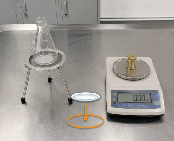
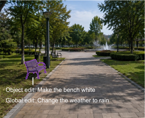

Dataset Statistics.
The 300 scenes include 266 snapshots and 34 expansion cases. Snapshot annotations cover 424 target objects and 72 support scenes. Thirty editing cases comprise 18 object edits and 12 global edits; these task-specific denominators must not be conflated.
4.2 Evaluation Metrics
W1 scores rendered quality, W2 geometry usability, W3 cross-view persistence, W4 editing with preservation, and W5 spatial expansion. Appearance comes from prescribed panoramas, paths, and object orbits; geometry and external simulation supply navigation and support evidence. W6 is unscored.
W1: Generative Construction.
Quality and preference models score rendered images, while CLIP measures conditioning alignment. Opacity-based coverage and requested-object detection add structural and semantic checks. Good aesthetic or embedding scores alone do not verify a correct world. [19] [83] [13]
W2: Interactive Simulation.
Navigation measures the largest connected traversable area relative to the footprint. A separate simulator tests whether plates remain on annotated surfaces. Traversal and reliable physical support are different capabilities.
W3: State Persistence.
Scene metrics assess valid viewpoints, brightness/hue stability, and location coverage combined with quality consistency. Object metrics combine visibility with appearance consistency, return-point tracking, or judged integrity. These composites penalize inaccessible views but do not establish full dynamic state simulation. [16] [113]
W4: Programmable Dynamics.
Editing requires both satisfying the instruction and preserving unrelated content. Success is a VLM judgment in any inspected post-edit view; background appearance and common-visible depth assess preservation. An instruction already satisfied before editing can pass the success test, so this is not strictly an improvement measure. [115] [73]
W5: Scalable Shared World.
Expansion scores footprint growth, additional rendered coverage, and view quality in new, original, and connecting regions. This is a restricted spatial-extension test; it does not demonstrate the full multi-agent shared-world capability proposed for W5.
Reporting.
Metric summaries are normalized to 0–100, with higher values better. Group scores equally average available retained metrics; missing values are excluded, measured failures remain, and untested groups show dashes. Appendix B specifies the differing denominators and frozen normalization.
4.3 Experimental Results
Read each group separately: the fixed table order is not a ranking valid across all metrics.
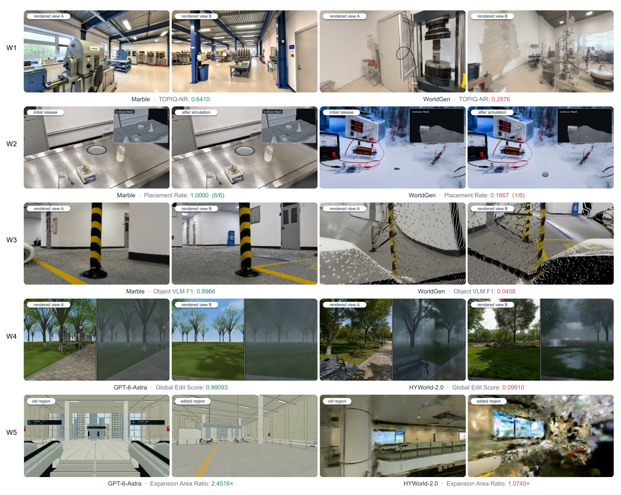
| Model | Arena Elo | W1 | W2 | W3 | W4 | W5 |
| GPT-6-Astra | 1252 | 63.72 | 65.43 | 68.80 | 82.09 | 63.10 |
| Marble | 1308 | 79.10 | 64.99 | 59.89 | 53.51 | 45.44 |
| HYWorld-2.0 | 1230 | 76.30 | 67.71 | 57.99 | 59.97 | 43.16 |
| HYWorld-1.0 | 1029 | 78.78 | 59.40 | 55.19 | 66.16 | - |
| Matrix-3D | 1019 | 46.35 | 56.35 | 52.73 | 49.76 | 35.15 |
| WorldGen | 962 | 69.17 | 60.11 | 54.16 | 57.56 | - |
| FlashWorld | 743 | 49.39 | 0.00 | 38.13 | - | - |
| Lyra 2.0 | 729 | 57.58 | 0.90 | 40.52 | - | - |
| Lyra 1.0 | 728 | 41.10 | 1.36 | 37.07 | - | - |
Overall performance across W1–W5.
Capability-adjusted spatial Elo ranks Marble first at 1308, GPT-6-Astra at 1252, and HYWorld-2.0 at 1230. Marble/HYWorld-1.0 lead appearance, HYWorld-2.0 leads physical usability, and GPT-6-Astra leads W3–W5 composites despite weaker W1 appearance. The Elo adjustment includes synthetic outcomes for unsupported capabilities, so it is not purely an observed human-vote ranking.
| Appearance quality | Coverage and alignment | |||||||||
| Model | TOPIQ | AES | PI | Q-Align | HPS | VLM | Hole-free ratio | CLIP-T | CLIP-I | Object coverage |
| GPT-6-Astra | 57.74 | 40.26 | 18.33 | 60.29 | 48.48 | 88.48 | 95.24 | 61.19 | 85.99 | 81.20 |
| Marble | 56.08 | 48.30 | 81.36 | 82.77 | 88.22 | 96.67 | 100.00 | 62.05 | 92.04 | 83.46 |
| HYWorld-2.0 | 42.82 | 46.76 | 73.70 | 78.73 | 80.81 | 95.47 | 99.95 | 62.23 | 93.85 | 88.72 |
| HYWorld-1.0 | 53.78 | 48.71 | 83.88 | 82.28 | 78.89 | 92.79 | 100.00 | 62.16 | 95.63 | 89.66 |
| Matrix-3D | 16.04 | 33.77 | 20.18 | 22.12 | 24.55 | 22.93 | 99.76 | 61.14 | 87.03 | 75.94 |
| WorldGen | 32.29 | 43.96 | 71.32 | 57.94 | 66.90 | 75.78 | 99.58 | 62.29 | 94.42 | 87.22 |
| FlashWorld | 44.84 | 40.84 | — | 38.50 | 12.15 | 37.97 | 25.61 | 59.68 | 94.66 | 90.23 |
| Lyra 2.0 | 36.11 | 40.45 | 69.13 | 45.22 | 50.31 | 30.80 | 71.74 | 61.39 | 89.06 | 81.58 |
| Lyra 1.0 | 39.92 | 41.12 | 0.00 | 34.35 | 6.23 | 34.58 | 18.32 | 59.21 | 91.71 | 85.53 |
W1: Observable quality.
Origin-centered panoramas favor representations that retain their initial appearance. Marble and HYWorld-1.0 lead overall W1; GPT-6-Astra's clean synthetic meshes score well on TOPIQ but lower on naturalness/preference. This favorable initial viewpoint does not test newly exposed geometry.
| Physical usability | ||
| Model | Navigable ratio | Placement rate |
| GPT-6-Astra | 69.05 | 61.81 |
| Marble | 65.17 | 64.81 |
| HYWorld-2.0 | 65.27 | 70.14 |
| HYWorld-1.0 | 51.90 | 66.90 |
| Matrix-3D | 64.09 | 48.61 |
| WorldGen | 68.83 | 51.39 |
| FlashWorld | 0.00 | 0.00 |
| Lyra 2.0 | 1.79 | 0.00 |
| Lyra 1.0 | 2.72 | 0.00 |
W2: Physical usability.
FlashWorld and the Lyra variants provide little navigable space and no successful placements under this protocol. Navigation and support rankings differ: HYWorld-2.0 has the best placement rate, 70.14%, while still failing some trials. These are outcomes under the paper's scale, geometry, and plate-support rules.
| Scene-level | Object-level | ||||||
| Model | In-bounds ratio | Brightness consistency | Hue consistency | Location HPS F1 | HPS F1 | Track F1 | VLM F1 |
| GPT-6-Astra | 98.05 | 90.01 | 90.70 | 62.04 | 28.16 | 47.34 | 65.27 |
| Marble | 96.62 | 86.58 | 88.70 | 54.25 | 24.83 | 39.27 | 28.96 |
| HYWorld-2.0 | 94.84 | 86.17 | 88.21 | 46.38 | 26.60 | 40.73 | 22.97 |
| HYWorld-1.0 | 96.01 | 80.04 | 82.35 | 39.79 | 23.45 | 42.40 | 22.28 |
| Matrix-3D | 94.55 | 87.02 | 87.94 | 56.61 | 18.17 | 18.38 | 6.44 |
| WorldGen | 87.70 | 80.80 | 83.82 | 46.76 | 21.59 | 33.17 | 25.30 |
| FlashWorld | 13.30 | 64.61 | 68.18 | 34.90 | 21.60 | 36.86 | 27.47 |
| Lyra 2.0 | 29.58 | 78.28 | 78.58 | 38.70 | 17.25 | 22.62 | 18.66 |
| Lyra 1.0 | 15.82 | 68.38 | 71.77 | 20.47 | 20.84 | 36.60 | 25.63 |
W3: Scene- and object-level persistence.
Stable brightness or hue can conceal broken object correspondence. Matrix-3D illustrates this separation, while GPT-6-Astra leads the scene and object composites. Cross-view identity and integrity therefore require checks beyond attractive or globally stable-looking renders.
| Execution | Object editing | Global editing | |||||
| Model | Succ. rate | BG RGB retention | BG LPIPS similarity | BG DINO similarity | Object score | Depth agreement | Global score |
| GPT-6-Astra | 60.00 | 100.00 | 99.12 | 99.82 | 66.55 | 99.57 | 49.57 |
| Marble | 56.67 | 90.08 | 7.86 | 89.29 | 40.50 | 55.08 | 35.08 |
| HYWorld-2.0 | 73.33 | 97.05 | 55.42 | 93.04 | 50.86 | 25.04 | 25.04 |
| HYWorld-1.0 | 66.67 | 99.61 | 94.86 | 99.27 | 54.98 | 24.34 | 23.36 |
| Matrix-3D | 40.00 | 97.89 | 43.73 | 93.41 | 19.90 | 32.46 | 20.93 |
| WorldGen | 56.67 | 98.96 | 89.30 | 98.46 | 32.65 | 15.83 | 11.03 |
W4: Controlled editing.
HYWorld-2.0 achieves the highest edit execution rate, 73.33%, but GPT-6-Astra leads preservation and both joint edit scores. A successful requested change can still damage the surrounding world.
| Growth and coverage | New region | Preservation | |||
| Model | Area score | Junction score | New-region quality | Old-region preservation | Path preservation |
| GPT-6-Astra | 39.71 | 67.48 | 72.56 | 52.54 | 83.20 |
| Marble | 17.48 | 55.33 | 74.00 | 28.28 | 52.12 |
| HYWorld-2.0 | 5.70 | 52.64 | 55.97 | 49.17 | 52.30 |
| Matrix-3D | 29.68 | 52.05 | 22.78 | 22.57 | 48.65 |
W5: Expansion with preservation.
Larger reconstructed footprints need not yield convincing new views or preserve old ones. GPT-6-Astra leads growth, junction improvement, and preservation; Marble leads new-view quality. Quality changes are evaluated at sampled views, not as a guarantee of unchanged geometry everywhere.
5 Embodied World Model Track
Each embodied test generates an egocentric robot video from an initial image and a natural-language action condition. W2 tests one action, W3 an ordered sequence, and W4 paired changes to actions or physical rules. Perception, consistency, causality, and controllability are scored separately. These are generated-video tests, not measured robot task success or numerical action-conditioned dynamics.
Equation 1
| (1) |
5.1 Data Construction
Only W2–W4 are operationalized in the embodied track; W1, W5, and W6 remain framework definitions.
Task Representation and Annotations
Task records contain identifiers, reference images, level, viewpoint, complete action prompts, and environment/subject annotations used to build evaluator assertions. W4 also records the shared intervention group and branch-specific condition.
Capability-Guided Case Design
W2 separates performing an atomic action from causing its intended effect. W3 checks ordered stages and accumulated state. W4 starts both branches from one image and changes an action property or a physical rule, then checks the required difference while preserving unrelated content.
Dataset Statistics
The formal set contains 62 W2 cases, 100 W3 cases, and 92 W4 matched intervention groups; each W4 group generates two branches. W2/W4 last 5 seconds and W3 lasts 12. Outputs are standardized to 24 FPS, then sampled at 4 FPS for scoring: 20 or 48 frames. The action vocabulary covers movement and diverse manipulation skills.
| Level | Cases | Rollout | Task composition |
| W2 | 62 | 5 s | Single-step robot actions with specified subjects, targets, directions, and post-action states. |
| W3 | 100 | 12 s | Ordered multi-step rollouts with explicit temporal stages and persistent robot, object, and scene states. |
| W4 | 92 | 5 s per branch | 40 action-condition pairs and 52 physical-rule pairs, each generated from one shared initial frame. |
| Total | 254 | — | 254 reference images and 2,768 rollout records. |
5.2 Evaluation Metrics
Seventeen metrics combine automatic visual measurements with fixed, task-specific VLM assertions. They include four perception, five consistency, three causality, and five controllability measures. Assertions carry predefined importance weights; inapplicable items are excluded rather than assigned zero.
Perception.
Scene and subject fidelity check recognizable input facts. MUSIQ-SPAQ measures perceptual quality; sharpness retention compares detail with the first generated frame.
Consistency.
Consistency evaluates masked robot appearance, static geometry, checkpointed scene/object state, motion-compensated visual continuity, and intermediate-frame predictability.
Causality.
Causality checks applicable physical constraints, the order of causes and effects, and whether visible changes have the prescribed triggers.
Controllability.
Controllability separates reaching an endpoint, performing the correct atomic action, producing its functional effect, ordering multiple actions, and distinguishing paired intervention branches. The overall weighting is 20% perception, 20% consistency, 30% causality, and 30% controllability. W4 branch fidelity contributes one score per matched group.
5.3 Experimental Results
Eight video generators are evaluated on the same embodied cases and judged with the same metrics and frozen assertions.
Experimental setup.
The candidates are MiniMax-H3, Cosmos 3, Seedance 2.5, Grok Imagine Video 1.5, HappyHorse 1.1, Kling 3, Sora 2, and Wan 3.0. Capability scores use a 0–100 scale. A blind, within-case human comparison provides a separate Arena Elo rating. [68] [69] [15]
Overall capability evaluation and human preference.
MiniMax-H3 leads all three overall capability scores and embodied Arena Elo. Cosmos 3 and Sora 2 stay below 75 at each level. Human preference broadly follows the automatic ordering, with local differences; neither measure alone establishes deployable robot competence.
| Model | Arena ELO | W2 | W3 | W4 |
| MiniMax-H3 | 1060 | 93.60 | 91.42 | 88.62 |
| Grok Imagine Video 1.5 | 1051 | 93.02 | 88.51 | 83.48 |
| Wan 3.0 | 1051 | 90.53 | 87.96 | 84.53 |
| Seedance 2.5 | 1031 | 90.91 | 86.73 | 84.11 |
| HappyHorse 1.1 | 1026 | 91.59 | 88.82 | 84.60 |
| Kling 3 | 978 | 85.94 | 84.26 | 78.70 |
| Cosmos 3 | 931 | 69.16 | 74.47 | 68.33 |
| Sora 2 | 872 | 60.91 | 65.35 | 64.12 |
W2: single-action execution.
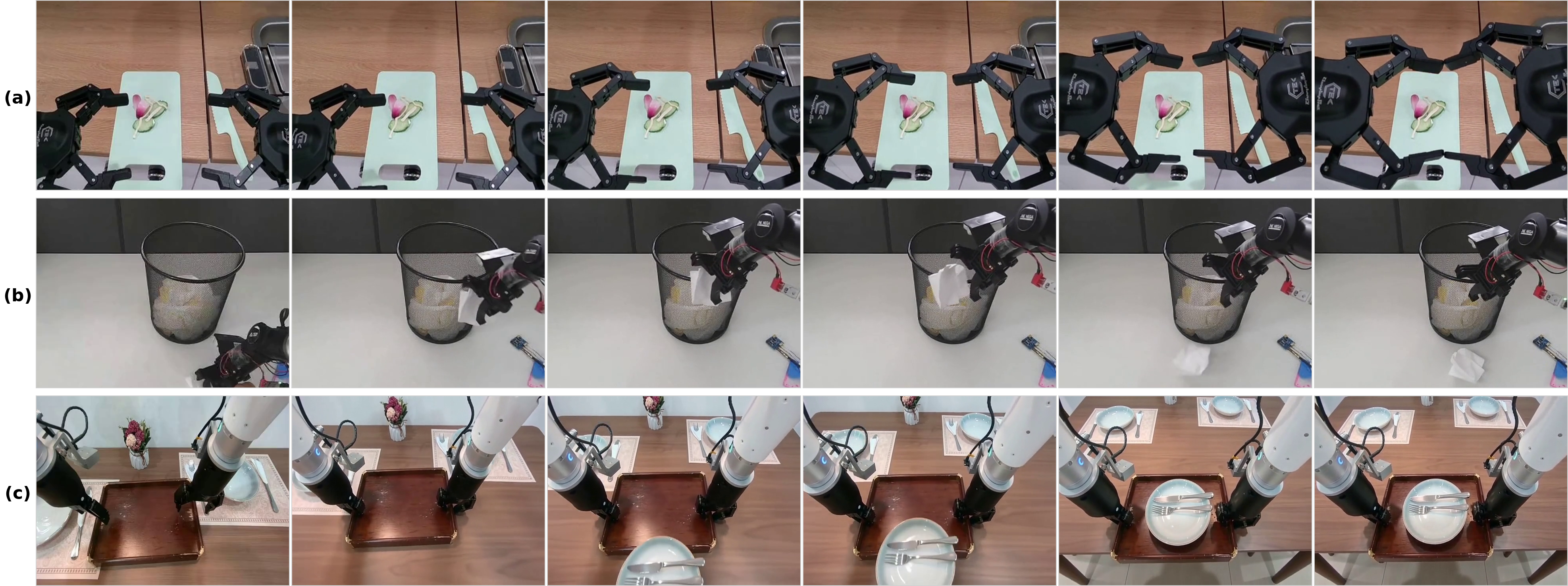
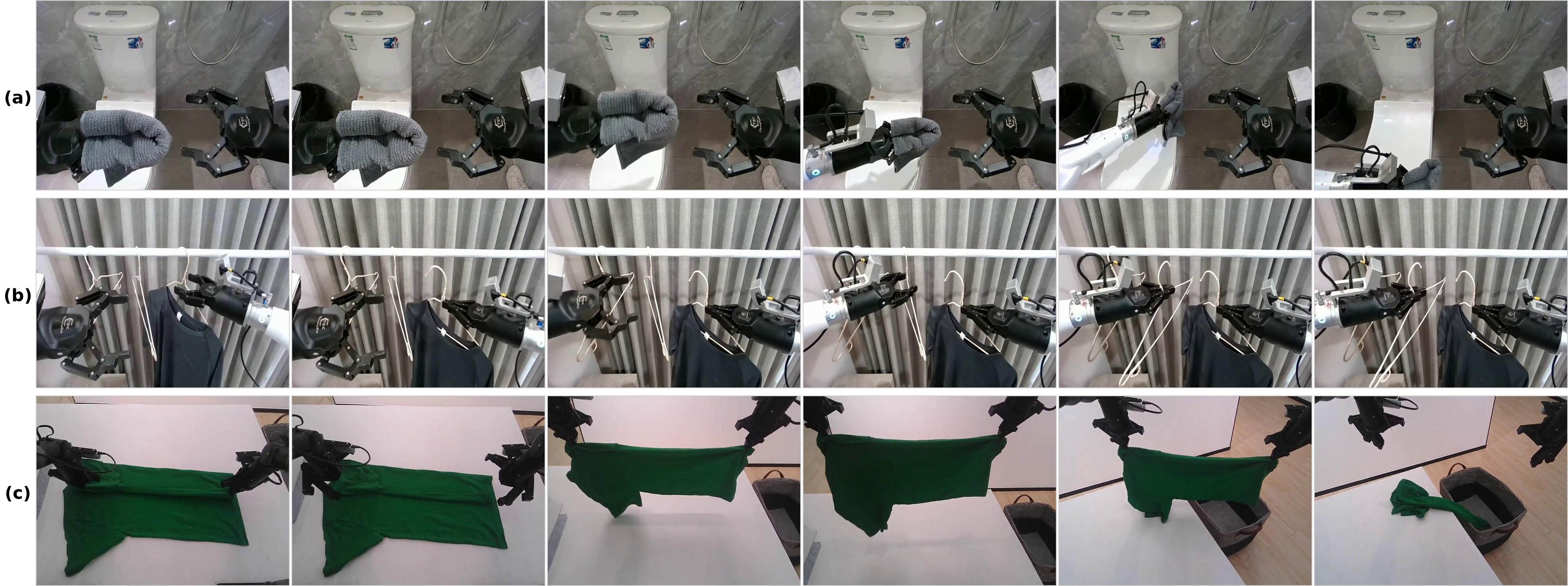
W2 failures include grasp-like gestures without contact, acting on the wrong object, and uncaused objects or camera changes. Other rollouts look plausible but miss the specified final placement. Correct execution requires the complete action–contact–effect–endpoint chain.
| Model | Perception | Consistency | Causality | Controllability | |||||||||||
| SF | SuF | PQ | SR | SAC | GC | SSC | TC | MS | PP | TCO | CTV | GSA | AAC | FIS | |
| MiniMax-H3 | 98.19 | 98.39 | 71.71 | 97.62 | 84.16 | 71.57 | 98.26 | 84.33 | 84.55 | 100.00 | 96.77 | 96.77 | 95.16 | 98.39 | 96.77 |
| Grok Imagine Video 1.5 | 97.96 | 98.79 | 73.32 | 98.37 | 89.53 | 70.52 | 98.42 | 79.54 | 80.77 | 94.62 | 96.77 | 96.77 | 95.16 | 98.39 | 96.77 |
| HappyHorse 1.1 | 98.19 | 98.59 | 70.45 | 94.72 | 88.38 | 69.57 | 98.28 | 77.43 | 79.02 | 98.92 | 95.16 | 95.16 | 91.94 | 93.55 | 95.16 |
| Seedance 2.5 | 98.19 | 98.79 | 70.22 | 95.96 | 90.03 | 74.93 | 98.40 | 88.72 | 89.09 | 97.85 | 90.32 | 90.32 | 88.71 | 91.94 | 91.94 |
| Wan 3.0 | 98.19 | 97.58 | 72.13 | 98.82 | 82.24 | 64.17 | 98.25 | 77.36 | 77.52 | 98.39 | 95.16 | 92.74 | 90.32 | 91.94 | 93.55 |
| Kling 3 | 97.96 | 98.79 | 71.40 | 99.10 | 90.02 | 71.34 | 97.46 | 79.39 | 76.43 | 97.85 | 85.48 | 84.68 | 75.81 | 79.03 | 87.10 |
| Cosmos 3 | 98.19 | 98.99 | 69.68 | 97.91 | 84.78 | 78.27 | 98.64 | 85.48 | 86.39 | 99.46 | 45.16 | 45.97 | 50.00 | 46.77 | 48.39 |
| Sora 2 | 89.56 | 89.52 | 64.97 | 95.06 | 88.40 | 66.82 | 88.23 | 83.81 | 84.89 | 90.86 | 40.32 | 37.10 | 37.10 | 30.65 | 38.71 |
W3: multi-action sequences with persistent state.
W3 exposes failed state transfer: an early stage may never create the required state, an intermediate result may be ignored, or later transport/placement may lose the intended outcome. A visually continuous sequence can therefore lack ordered, accumulated effects.
| Model | Perception | Consistency | Causality | Controllability | ||||||||||||
| SF | SuF | PQ | SR | SAC | GC | SSC | TC | MS | PP | TCO | CTV | GSA | AAC | FIS | MAO | |
| MiniMax-H3 | 99.17 | 98.42 | 70.17 | 91.90 | 88.14 | 51.30 | 98.72 | 72.85 | 72.30 | 99.67 | 97.00 | 94.38 | 97.00 | 96.33 | 96.33 | 97.00 |
| HappyHorse 1.1 | 98.91 | 98.92 | 68.80 | 85.32 | 84.25 | 46.65 | 97.26 | 66.62 | 68.04 | 98.08 | 95.33 | 93.12 | 92.00 | 94.08 | 92.67 | 95.33 |
| Grok Imagine Video 1.5 | 98.98 | 98.75 | 73.53 | 93.19 | 84.77 | 40.24 | 95.92 | 56.94 | 56.58 | 95.92 | 95.50 | 95.00 | 94.00 | 93.42 | 94.00 | 95.50 |
| Wan 3.0 | 99.32 | 98.40 | 71.28 | 93.95 | 86.84 | 43.54 | 96.66 | 69.49 | 70.31 | 96.33 | 93.00 | 89.38 | 89.00 | 90.25 | 91.83 | 92.50 |
| Seedance 2.5 | 99.62 | 98.50 | 68.07 | 84.48 | 86.09 | 52.74 | 98.73 | 76.73 | 77.07 | 97.00 | 88.00 | 88.12 | 84.50 | 87.83 | 88.33 | 89.00 |
| Kling 3 | 99.05 | 98.66 | 71.73 | 98.22 | 87.09 | 56.71 | 98.06 | 73.64 | 71.52 | 94.83 | 82.33 | 86.25 | 81.00 | 78.42 | 79.67 | 81.67 |
| Cosmos 3 | 99.34 | 98.67 | 70.36 | 97.39 | 86.74 | 63.10 | 98.24 | 81.69 | 82.35 | 96.58 | 56.67 | 68.12 | 55.50 | 62.42 | 60.00 | 56.17 |
| Sora 2 | 93.30 | 95.75 | 63.92 | 87.06 | 83.73 | 56.62 | 93.22 | 75.06 | 77.23 | 90.83 | 49.83 | 46.25 | 38.00 | 52.17 | 49.33 | 50.17 |
W4: rule editing under a shared initial state.
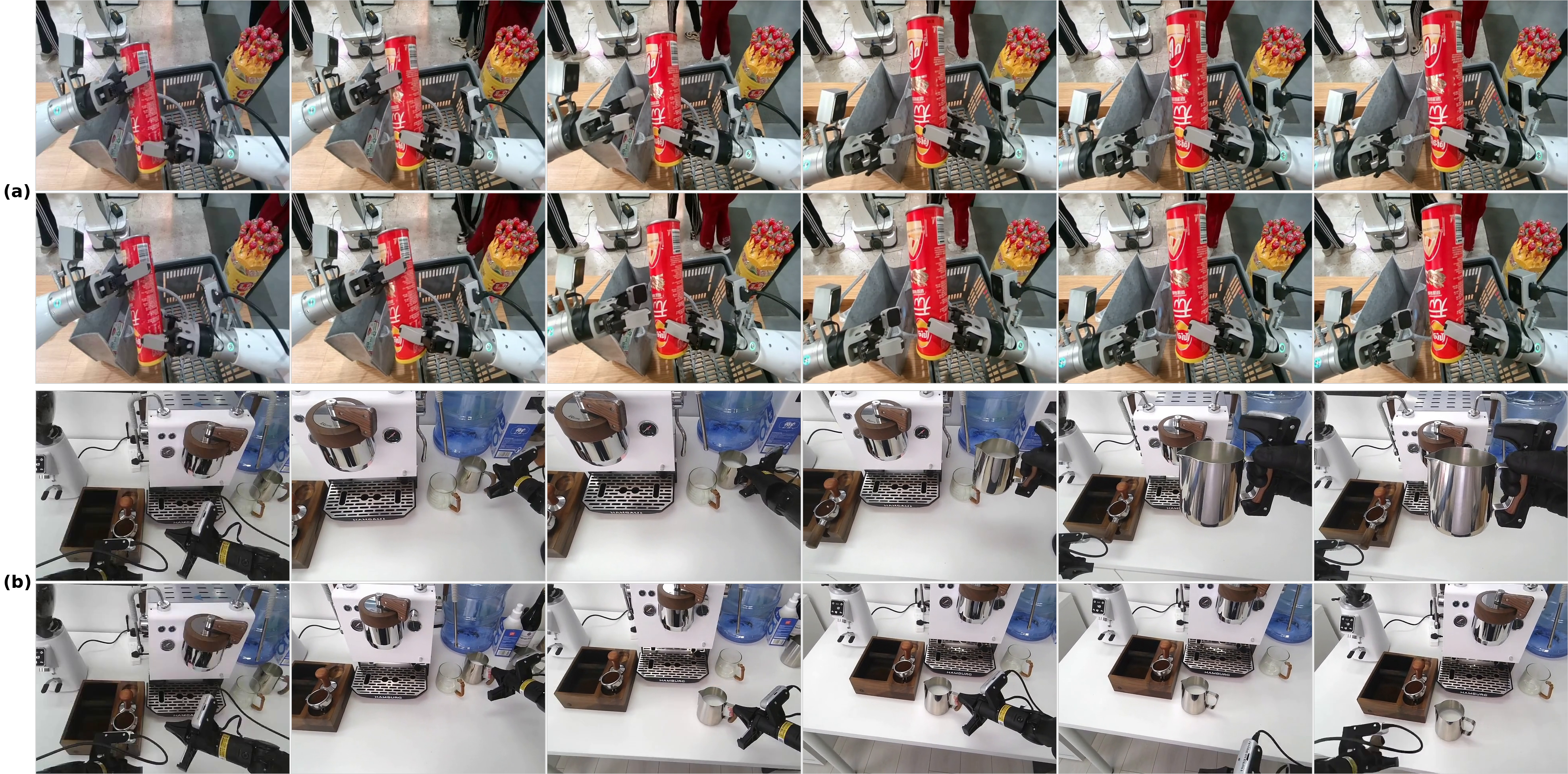
W4 often shows little visible response to altered gravity, friction, or material rules. Action edits can influence the rough outcome while changing the required interaction—for example, dragging instead of pushing. Successful paired videos must reflect the edited condition and preserve their shared unaffected state.
| Model | Perception | Consistency | Causality | Controllability | |||||||||||
| SF | SuF | PQ | SR | SAC | GC | SSC | TC | MS | PP | TCO | CTV | GSA | FIS | CBF | |
| MiniMax-H3 | 98.91 | 97.69 | 71.44 | 96.40 | 88.81 | 69.73 | 98.17 | 78.09 | 76.11 | 97.15 | 89.13 | 89.67 | 87.50 | 88.75 | 87.39 |
| HappyHorse 1.1 | 98.97 | 98.06 | 69.31 | 85.69 | 84.42 | 48.98 | 95.05 | 59.54 | 60.80 | 95.29 | 86.41 | 85.87 | 86.41 | 85.00 | 91.52 |
| Wan 3.0 | 98.56 | 98.25 | 71.87 | 95.38 | 86.74 | 55.37 | 96.09 | 65.61 | 64.98 | 92.03 | 83.70 | 85.33 | 83.15 | 90.00 | 81.52 |
| Seedance 2.5 | 98.83 | 98.19 | 69.62 | 90.91 | 87.65 | 64.37 | 97.91 | 77.00 | 75.92 | 94.11 | 82.61 | 80.43 | 79.35 | 82.50 | 82.17 |
| Grok Imagine Video 1.5 | 98.88 | 97.28 | 73.39 | 95.57 | 84.82 | 48.30 | 92.98 | 48.75 | 47.18 | 88.99 | 86.96 | 85.87 | 86.41 | 90.00 | 85.22 |
| Kling 3 | 98.77 | 96.58 | 71.21 | 97.63 | 88.65 | 66.01 | 96.47 | 70.97 | 67.07 | 87.27 | 70.11 | 74.46 | 65.22 | 75.00 | 77.17 |
| Cosmos 3 | 99.12 | 97.26 | 70.54 | 97.48 | 87.80 | 74.35 | 98.01 | 82.12 | 82.37 | 89.72 | 45.11 | 48.37 | 44.02 | 47.50 | 56.52 |
| Sora 2 | 93.95 | 94.03 | 64.34 | 91.59 | 87.47 | 65.54 | 93.12 | 75.30 | 76.76 | 84.01 | 42.93 | 42.39 | 40.22 | 41.25 | 59.13 |
Cross-level capability analysis.
Across the three levels, visual fidelity is stronger than action grounding, persistent state evolution, and precise conditional response. The tests diagnose these weaknesses within this benchmark; their distinct case pools and interfaces do not isolate a single causal source of failure.
6 Conclusion
The contribution is a common evaluation vocabulary plus complementary human and automatic measurements. The study supports checking behavior and preservation alongside visual quality. Its current tests cover selected capabilities with learned evaluators and adapted interfaces; they do not certify universal world modeling, downstream planning, or real robot reliability.
Paper identity
The author list is alphabetical. Affiliations include Alibaba Token Hub, BIGAI, Tsinghua University, Nanjing University, and Peking University. The original first-page marks and HappyWorld-Arena link are retained below.



Appendix A Video World Model Track
Appendix A records the evaluated video interfaces and exact metric formulas.
A.1 Inference Protocols and Model Configurations
Model inputs, temporal discretization, image preprocessing, and available controls differ. These adaptations are part of the measured systems and must accompany their scores.
Genie 3 via Project Genie.
Genie 3 is tested through hosted Project Genie, including its world-creation components, using browser-scheduled keys. Inputs are resized without cropping or generative enhancement; descriptions may be truncated. Checkpoint, seed, and sampling settings are unavailable. Export timing permits ±5 seconds and operational failures are retried without score-based selection. Only supported W1–W3 cases are evaluated, so this characterizes the deployed service rather than an isolated checkpoint. [74] [75]
HappyOyster.
HappyOyster uses one configuration across cases, with image aspect ratio preserved near an 832×480 pixel budget and dimensions rounded to multiples of 16. Timed translation/camera controls are aligned to frames, simultaneous commands combine, and causal state continues within each independently initialized rollout. [5]
Lingbot-World-v2
LingBot-World-v2 uses a distilled causal model with camera poses encoded through Plücker geometry, approximately 832×480 output at 16 FPS. Event-only descriptions become a single global prompt with a fixed camera, rather than timed prompt updates; this limits intervention timing even though the model enters the W4 comparison. [33]
MatrixGame-2.0
Matrix-Game 2.0 uses image conditioning and framewise keyboard/mouse controls at 640×352 and 12 FPS. It ignores textual scene/role/event descriptions; event-only cases become zero-control rollouts and therefore do not implement their requested interventions. [39]
MatrixGame-3.0
Matrix-Game 3.0 combines text/image conditioning, keyboard/mouse signals, and camera-pose embeddings at 1280×704 and 16 FPS. Natural-language events are omitted, so zero-control cases retain scene descriptions but do not execute timed W4 edits. [95]
Yume-1.5
Yume-1.5 uses the 5B model with an InternVL-refined prompt and a structured camera-control vocabulary. Intervals are rounded to 29-frame chunks, about 1.81 seconds at 16 FPS; output is 1280×704. Unexpressible event-only/no-discrete-control cases are not evaluated, and arbitrary W4 language edits are unsupported in this adaptation. [65] [21]
DreamX-World 1.0
DreamX-World 1.0 converts controls into relative camera poses and PRoPE conditioning, producing 1280×704 video at 16 FPS. Text stays fixed and there is no independent character control. Event-only cases are not generated, so the evaluation does not implement language-based interventions. [26]
ABot-World
ABot-World-0-5B streams half-second blocks with binary translation/rotation keys and a persistent KV cache. Outputs are resampled to the requested duration at 832×480 and 12 FPS. Fixed scene text excludes event instructions; zero-control rollouts do not implement timed W4 edits. [46]
Cosmos3
Cosmos3 Nano uses the autonomous-driving action domain because the authors found its explicit camera-pose interface unreliable on these scenes. Lateral commands become curved strafes, pitch is dropped, and turning in place adds forward motion. Sessions continue from prior final frames, producing 16 FPS video with a 480-pixel short side. Event-only cases are skipped. These control approximations materially qualify its comparison. [1]
JoyAI-Echo
JoyAI-Echo's Flash model encodes timed keys as a smoothed camera trajectory with UCPE conditioning, producing 1280×704 video at 24 FPS. Released controls may leave residual movement. Event-only text enters a global prompt; when movement controls exist it is omitted, so timed language interventions are not implemented. [117]
Alaya-EVOKE
Alaya-EVOKE converts local movement and camera rotation into a trajectory sampled at 30 FPS and consumed at 24 FPS. It uses the released distilled checkpoint, three pyramid steps, and no classifier-free guidance, at 640×384. Its chunk-based frame-count rule can differ from exact requested duration. [108]
Lyra 2.0
Lyra 2.0 uses camera trajectories and fixed scene text at 832×480 and 16 FPS. Third-person controls move a proxy subject position around which the camera looks; they do not independently control a character. DA3 geometry and MoGe depth-scale alignment initialize the scene. [87]
SANA-WM
SANA-WM takes text, a center-cropped 1280×704 reference, and framewise camera poses at 16 FPS. The flow-DPM sampler runs 60 steps with shift 9.8; the LTX-2 refiner and control overlays are disabled. The same scene prompt conditions the rollout. [124]
Open-Oasis
Open-Oasis uses image conditioning and a 25-component action vector at 640×360 and 20 FPS. Camera-axis magnitudes are 0.1; inference uses FP32 and ten DDIM steps per generated frame. [23]
A.2 Detailed Metrics
Video metrics span perception, consistency, causality, and control. Most normalized scores are reported on a 0–100 scale, while raw preference or motion measures require their own interpretation. Missing or inapplicable measurements are omitted, and identical abbreviations can denote different metrics in another track.
A.2.1 Perception and Representation
These metrics assess frame quality, image stability, visible motion, and initial instruction fidelity.
Imaging Quality (VQ).
VQ averages normalized MUSIQ frame-quality scores. Clean images can still be temporally, physically, or semantically wrong.
Equation 2
| (2) |
Human Preference Score v3 (HPS).
HPS averages HPSv3 rewards after clipping frame outliers at the first and 99th percentiles. It estimates preference rather than instruction compliance or causal correctness; its reward scale is not a probability.
Equation 3
| (3) |
Brightness Consistency (Bri).
Bri compares coarse grayscale histograms with the initial frame through a nonlinear similarity transform. It ignores spatial arrangement and can penalize intentionally changed lighting.
Equations 4–5
| (4) |
| (5) |
Color-Temperature Consistency (CT).
CT compares seven-bin hue histograms with both the first and preceding frames. It measures palette stability, not localized color errors or physical temperature.
Equation 6
| (6) |
Sharpness Retention (SR).
Video SR compares summed Sobel edge descriptors with the first frame. After three sufficiently noisy BRISQUE assessments, the current and all later similarity scores become zero. It measures retention relative to the starting image, not absolute detail quality.
Equation 7
| (7) |
Imaging Stability (IS).
IS equally averages brightness, color-temperature, and sharpness-retention scores after normalization.
Equation 8
| (8) |
Dynamic Degree (Dyn).
Dyn aggregates RAFT flow magnitudes to describe motion amount. Large motion need not be smooth, commanded, or physically correct.
Equation 9
| (9) |
Instruction Following (IF).
IF averages applicable atomic requirements, using binary or normalized ordinal rubrics. For W4 it checks only the initial world before intervention, so a requested later change is not penalized as initial-instruction failure.
Equations 10–11
| (10) |
| (11) |
A.2.2 Consistency and State Retention
Consistency metrics distinguish background appearance, geometry, texture, state, and subject identity.
Background Consistency (BC).
BC masks the moving subject and compares CLIP background features at 3 FPS, combining adjacent and initial-frame similarity. These masked scores are not directly comparable to standard full-frame background consistency.
Equation 12
| (12) |
Object Geometry Consistency (GC).
Video GC uses DA3 depth and estimated poses to test cross-frame geometric reprojection. It assesses estimated structural agreement, not simply image similarity.
Equation 13
| (13) |
Texture Consistency (TC).
Video TC measures aligned surface appearance through a PSNR-style photometric residual, using the same estimated correspondences as GC.
Equation 14
| (14) |
State Consistency (SC).
SC maps a five-level judgment of persistent states and justified changes to a normalized score. It differs from WorldMark's official LPIPS/DINOv2 procedure, so their numbers should not be mixed.
Equation 15
| (15) |
Subject Consistency (SuC).
SuC isolates the subject with SAM2.1, then combines adjacent DINOv2 similarity and long-range CLIP similarity on standardized crops.
Equation 16
| (16) |
A.2.3 Causality and Causal Rollout
These checks require visible evidence of physical or event relationships rather than plausible-looking final frames.
Physical Causality (PC).
PC scores applicable physical-process assertions from one to five, normally requiring at least two assessable items. Invisible prerequisites can be inapplicable; visible incorrect behavior remains a failure.
Equation 17
| (17) |
Content Causality (CC).
CC similarly scores explicit trigger–consequence chains for order, outcome, and persistence. Co-occurrence alone is insufficient, and the default minimum is two applicable assertions.
Equation 18
| (18) |
Interpenetration (IP).
IP averages binary judgments that relevant contact/support relations avoid penetration or unsupported floating. This is a visual interaction check, not complete 3D collision simulation.
Equation 19
| (19) |
A.2.4 Controllable Interaction and Counterfactuals
Control metrics separate camera direction, action completion, admissible intervention processes, and persistent intended outcomes.
Trajectory Accuracy (TA).
TA compares commanded translation direction with DA3-estimated segment displacement; zero motion fails. It does not measure exact travel distance, speed, position, or camera rotation.
Equations 20–22
| (20) | ||||
| (21) | ||||
| (22) |
Action Execution (AE).
AE checks visible completion of time-aligned W2–W3 action requirements. Missing actors, absent targets, incorrect actions, and unmet states count as failures rather than exclusions.
Equation 23
| (23) |
Interaction Validity (IV).
W4 IV scores whether intervention follows valid contact, support, continuity, and other causal constraints. It deliberately leaves target achievement and preservation to SF, avoiding duplicate penalties.
Equation 24
| (24) |
State Fidelity (SF).
Video SF balances achievement, persistence, and preservation subclasses. Averaging within each subclass before combining them prevents numerous achievement items from dominating the other requirements.
Equation 25
| (25) |
Appendix B Spatial World Model Track: Detailed Metrics
Appendix B defines 39 spatial quantities, of which 31 enter the reported W1–W5 tables after consistency/coverage components are replaced by composites. Operation-specific preservation stays under editing or expansion; W6 remains unscored.
| Group | IDs | Number |
| Observable Quality (W1) | M01–M07, M09–M11 | 10 |
| Physical Usability (W2) | M08, M25 | 2 |
| Scene/Place Consistency (W3) | M12–M15, M38–M39 | 6 |
| Object Consistency (W3) | M16–M24 | 9 |
| Controlled Editing (W4) | M31–M37 | 7 |
| Expansion and Preservation (W5) | M26–M30 | 5 |
| Unified World Model (W6): unscored | None | 0 |
B.1 Shared Notation, Actions, and Evaluation Inputs
Spatial formulas use rendered RGB, depth, opacity, camera poses, and a harmonic combination of paired components. Dispersion uses population standard deviation. Empty conditional sets are undefined; absent targets have zero recall/composites, while evaluator unavailability is a separate status.
Equations 26–27
| (26) |
| (27) |
Camera sampling for W3 consistency.
The exposed state includes the observer pose, so moving through a static reconstruction changes observations. Local translation uses a 1 m/s convention; panoramas and object orbits are separate inspection cameras. Following prescribed poses does not independently demonstrate learned dynamics, pose-estimation accuracy, or action latency.
Equations 28–29
| (28) |
| (29) | ||||
Coordinates, scale, and geometry.
The initial camera defines right/forward/up coordinates. Nine downward rays anchor scale where possible; otherwise a depth percentile is assigned a five-meter scale. These are conventions, not recovered real dimensions. Cleaned geometry and footprints share a 0.05 m grid, with the same original transform retained before/after edits or expansion.
Equation 30
| (30) |
Common execution procedure.
The complete source procedure below fixes import, normalization, cached viewpoints, rendering, and evaluation records.
-
Import the representation, retain the source asset, and log any geometry conversion.
-
Establish coordinates and scale, recording the selected normalization branch.
-
Cache origin views and six-face probes, action trajectories, orbit cameras, and task annotations.
-
Render RGB/depth/raw opacity; construct cleaned collision geometry and common-grid footprints.
-
Evaluate eligible tasks with frozen scorers and preserve components, counts, and failure statuses.
B.2 W1: Generative Construction
Ten W1 measures average prescribed origin views, subject to each metric's sampling rule. Checkpoints, prompts, resolution, field of view, and rendering settings form part of the metric definition.
M01. topiq_nr ( ↑ ).
M01 averages the frozen TOPIQ-KonIQ quality regressor. Its learned output need not be a bounded probability. [19]
Equation 31
| (31) |
M02. laion_aes ( ↑ ).
M02 applies a learned aesthetic head to normalized CLIP embeddings and averages frames. Aesthetic appeal does not verify scene correctness. [83]
Equation 32
| (32) |
M03. pi ( ↓ ).
M03 combines Ma quality prediction with NIQE naturalness to form PI. It requires the specified feature pipeline and checkpoints; it is not simply NIQE alone. [13]
Equations 33–34
| (33) |
| (34) |
M04. q_align ( ↑ ).
M04 converts Q-Align logits over five quality labels into their expected score, then averages frames. Under this formulation the raw range is one to five. [97]
Equation 35
| (35) |
M05. hpsv3 ( ↑ ).
M05 averages text-conditioned HPSv3 rewards using a frozen prompt/checkpoint. Rewards can be negative; HPSv2 is not an equivalent replacement. [64]
Equation 36
| (36) |
M06. vlm_score ( ↑ ).
M06 averages Qwen3-VL binary judgments of artifact freedom, sharpness, and plausible layout across 18 prescribed views, retaining the component rates. [8]
Equation 37
| (37) |
M07. hole_rate ( ↓ ).
M07 measures pixels below 0.5 raw opacity before background compositing. It detects missing rendered coverage, not watertight geometry: a wrong opaque wall can score well and intentional sky can count as a hole.
Equation 38
| (38) |
M09. clip_t ( ↑ ).
M09 averages CLIP text–image cosine similarity across origin views. It measures broad semantic alignment rather than exhaustive object/relation correctness. [79]
Equation 39
| (39) |
M10. clip_i ( ↑ ).
M10 averages the three origin views most similar to the input image in CLIP space. Best-view selection reduces orientation mismatch but does not measure fidelity of the entire world.
Equation 40
| (40) |
M11. object_coverage ( ↑ ).
M11 unions category detections across six origin probes and divides by requested categories. Missing annotated categories fail; an empty annotation is inapplicable. Counts of individual instances are not checked.
Equation 41
| (41) |
B.3 W2: Interactive Simulation
W2 tests geometry through Habitat-Sim navigation and externally simulated plate support, rather than a learned scene's own dynamics. [35]
M08. navigable_ratio ( ↑ ).
M08 divides the largest four-connected rasterized NavMesh component by scene footprint area; it need not contain the starting observer. The agent has 0.1 m radius, 1.5 m height, 0.2 m step height, and 45° slope limit. Failed fine-grid builds retry coarser grids with settings recorded; empty footprints are invalid.
Equation 42
| (42) |
M25. tabletop_ready_rate ( ↑ ).
M25 requests six plate placements per annotated support and averages retained trials. Missing usable geometry/support/locations score zero; unavailable runs remain missing. A 0.22 m plate is released for five seconds in PyBullet. Success depends on penetration, vertical drop, and remaining within the support boundary; displacement and tilt are recorded but do not determine success. Thus the metric has a specific support predicate, not an unrestricted stability guarantee.
Equation 43
| (43) |
B.4 W3: State Persistence
W3 includes six scene-level and nine object-level diagnostics of observations under changing viewpoints.
B.4.1 Scene-Level (Place) Metrics
Scene metrics describe valid camera locations, appearance continuity, and quality consistency across sampled places; they do not independently test movement-direction accuracy.
M12. oob_ratio ( ↓ ).
M12 combines six-face hole coverage, footprint membership, and depth-based clearance into an invalid-view proxy. Without a footprint it falls back to the hole criterion; metric scale is needed for the clearance check.
Equations 44–45
| (44) | ||||
| (45) |
M13. brightness_consistency ( ↑ ).
M13 compares three-bin brightness histograms with the initial view, including out-of-bounds frames, using a fixed nonlinear transform. Rearranged objects can retain a similar global histogram.
Equations 46–47
| (46) |
| (47) |
M14. color_temperature_constraint ( ↑ ).
M14 compares seven-bin hue histograms with initial and adjacent views. All pixels contribute without a saturation mask; this measures palette continuity rather than kelvin temperature.
Equation 48
| (48) |
M15. place_hpsv3_std ( ↓ ).
M15 measures population standard deviation of mean HPSv3 rewards at the origin and accepted locations. Four depth-scaled radii each permit two locations; unused quotas do not transfer. At least one additional scored location is required, and rejected positions do not enter dispersion.
Equation 49
| (49) |
M38. place_recall ( ↑ ).
M38 has eight non-origin location slots. The implemented reported recall counts accepted, successfully scored locations, so it can include evaluator failures as well as geometric accessibility. Absent/unavailable sections remain missing, but certain failed sections—including a failed origin—produce zero.
Equations 50–51
| (50) |
| (51) |
M39. place_hpsv3_f1 ( ↑ ).
M39 combines inverse HPS dispersion with the same scene's reported location recall before averaging scenes. Its 'precision' is an inverse-dispersion proxy, not true-positive precision: uniformly poor views can appear consistent. Zero recall yields zero; different valid populations can complicate model-level component comparisons.
Equation 52
| (52) |
Action-path algorithm.
The complete path procedure preserves camera requests, usability outcomes, sampled-location membership, and component validity alongside the six metrics.
-
Reset to the original observer pose and load the timed action/camera manifest.
-
Apply each movement step, render its observation, and retain requested and realized poses when available.
-
Construct the eight-location plan, retain every usability outcome, and calculate M38.
-
Return six metrics, sampled cameras, quality-set membership, valid counts, and execution status.
B.4.2 Object-Level Metrics
Each object uses 24 fixed-radius orbit views without camera rejection or radius search. Visibility failures may arise from geometry, occlusion, camera placement, or segmentation.
M16. obj_sam_recall ( ↑ ).
M16 counts SAM3-visible orbit views, returning zero when fewer than two detect the target and otherwise dividing by 24. This is detected-view coverage, not recall against exhaustive ground-truth masks. [16]
Equation 53
| (53) |
M17. obj_hpsv3_std ( ↓ ).
M17 measures HPSv3 dispersion on masked object crops with background replaced by mean target color. Crops use eight-pixel padding; masks below 64 pixels are excluded and at least two scored crops are required.
Equation 54
| (54) |
M18. obj_hpsv3_f1 ( ↑ ).
M18 harmonically combines inverse object-quality dispersion with SAM visibility coverage. Consistently low quality can still receive a high consistency component; the scale depends on the frozen reward model.
Equation 55
| (55) |
M19. obj_track_accuracy ( ↑ ).
M19 tracks 64 target points around a 24-view orbit and repeats the initial image as frame 25. Endpoint agreement is normalized by object size. The repeated start can hide intermediate drift, so this is not full-path stationarity. [113]
Equation 56
| (56) |
M20. obj_track_f1 ( ↑ ).
M20 combines per-object endpoint tracking accuracy and visible-view coverage before averaging. Positive coverage with unavailable tracking is excluded; zero coverage contributes zero even without tracking.
Equation 57
| (57) |
M21. obj_vlm_recall ( ↑ ).
M21 asks Qwen3-VL whether each orbit view is inside the scene with a present, unoccluded target, then divides valid views by 24. It has no two-view minimum and is judged visibility rather than ground-truth recall.
Equation 58
| (58) |
M22. obj_vlm_artifact_free ( ↑ ).
M22 averages artifact-free judgments only over valid views, checking defects such as floaters, blur, stretching, holes, duplication, and melting. No valid views leaves the conditional score undefined.
Equation 59
| (59) |
M23. obj_vlm_completeness ( ↑ ).
M23 judges visible completeness over the same valid views. It is not reconstructed-surface recall against a reference scan; empty valid sets remain undefined.
Equation 60
| (60) |
M24. obj_vlm_f1 ( ↑ ).
M24 combines mean conditional artifact freedom/completeness with valid-view coverage. Its retained components distinguish poor visibility from poor visible integrity.
Equation 61
| (61) |
Object algorithm.
The source algorithm retains all nine object outputs together with segmentation masks, tracks, annotations, valid counts, and error states.
-
Render the 24 fixed orbit views and apply SAM3 to every view.
-
Compute ; if positive, compute masked HPS dispersion and , otherwise set .
-
Build the repeated-start tracking sequence and compute where evaluable; form with the zero-recall rule.
-
Judge every view’s validity; compute and conditional integrity components.
-
Set when ; otherwise combine components.
-
Store all nine outputs, annotations, masks, tracks, valid counts, and error states.
B.5 W4: Programmable Dynamics
W4 compares worlds from identical pre-edit cameras. Allowed-change masks depend on addition, deletion, replacement, or modification; their complement defines preserved background. Missing target masks fall back to the whole image. These tests cover restricted visual editing, not independently verified programming of physical laws or causal mechanisms.
M31. Edit success rate ( edit_execution , ↑ ).
M31 gives an edit case one if any selected post-edit view satisfies the instruction. No located object views score zero. Before-edit judgments do not require improvement, so an already-satisfied no-op can pass.
Equation 62
| (62) |
M32. rgb_psnr_bg ( ↑ ).
M32 averages valid background PSNR values within each case, then transforms that mean for the joint object score. It is not equivalent to first averaging per-frame reconstruction errors; frames require at least 64 background pixels.
Equations 63–65
| (63) | ||||
| (64) |
| (65) |
M33. lpips_bg ( ↓ ).
M33 averages the spatial LPIPS-VGG distance map over the background, without mask dilation. Whole-image scalars or blacked-out targets are not equivalent. Feature receptive fields can cross the allowed-edit boundary. [115]
Equation 66
| (66) |
M34. dinov2_bg_distance ( ↓ ).
M34 compares normalized DINOv2 patch features after resizing to 518×518. Background coverage must exceed one half for a patch; at least four patches are required per frame. [73]
Equation 67
| (67) |
M35. depth_agree_ratio ( ↑ ).
M35 compares before/after depth only where both renders have valid opacity and depth, averaging qualifying frames equally. Removed geometry outside this common-visible mask is not penalized by the depth score.
Equations 68–69
| (68) |
| (69) |
M36. edit_score_object ( ↑ ).
M36 combines each object edit's binary success and preservation components before model averaging. Raw case scores can lie outside 0–1 and are clipped only during table normalization. Failed execution yields zero; successful execution with missing preservation yields a missing composite.
Equation 70
| (70) |
M37. edit_score_global ( ↑ ).
M37 combines edit success and depth preservation for each global-edit case. It inherits the no-op and common-visible-mask limitations and uses a different population/function from the object-edit score.
Equation 71
| (71) |
Editing algorithm.
The full editing procedure below preserves the success and preservation components separately. Changing material appearance does not establish changed simulator friction or mass.
-
Freeze pre-edit coordinates/cameras and select views for judging edit success by operation type.
-
Judge before/after instructions and apply the any-after-view rule.
-
For global edits, evaluate M35 on paired common-valid geometry.
B.6 W5: Scalable Shared World
W5 uses common-grid before/after footprints and samples at the centroid of newly occupied cells. Identical original, junction, and connecting-path cameras support paired comparisons. The test measures spatial growth and sampled-view quality, not arbitrary shared multi-agent interaction.
M26. expand_area_ratio ( ↑ ).
M26 divides total footprint area after expansion by area before expansion. A raw ratio of one means unchanged area; old cells can disappear despite net growth. Case ratios are averaged rather than pooling areas.
Equation 72
| (72) |
M27. junction_coverage_gain ( ↑ ).
M27 measures paired improvement in opacity coverage at shared junction cameras. More rendered content does not establish correct surfaces or traversable connectivity.
Equation 73
| (73) |
M28. new_region_hpsv3 ( ↑ ).
M28 scores new-region proxy views with frozen HPSv3. It is not a uniform quality sample over all newly created cells.
Equation 74
| (74) |
M29. old_region_hpsv3_delta ( ↑ ).
M29 measures the change in HPSv3 at the original viewpoints. Equal preference rewards do not prove unchanged geometry or object identity.
Equation 75
| (75) |
M30. connect_hpsv3_delta ( ↑ ).
M30 averages before/after HPSv3 differences along 16 connecting-path frames. It describes changes in view quality along that selected route.
Equation 76
| (76) |
Expansion algorithm.
The complete expansion procedure retains paired components, camera locations, sample counts, and failure statuses. Published table scores apply the normalization described below rather than displaying raw area ratios or signed reward changes.
-
Reuse the original coordinate/scale transform for both worlds and rasterize common-grid footprints.
-
Locate the center of newly occupied cells and set its camera height using the expanded ground and original camera height.
-
Freeze origin, junction, and connecting-path cameras.
-
Return paired components, selected locations, sample counts, and failure statuses.
B.7 Aggregation and Reproducibility
Aggregation preserves the hierarchy of frames, objects/cases, composites, and models, along with metric-specific validity.
Aggregation and missingness.
Calculate components and nonlinear composites within each object or case before model averaging. Keep nominal scenes, objects, support trials, and operation subsets distinct. Unsupported, untested, invalid, and measured-zero statuses have different meanings; absent annotated targets must not disappear as unevaluable successes.
Equation 77
| (77) |
Evaluation settings.
Reproducibility requires fixed scorers, transforms, navigation connectivity, placement criteria, object crops, edit masks, and expansion viewpoints. Reports retain component values, valid counts, and failure statuses.
Interpretation.
The spatial results are descriptive averages for the specified operations. They do not directly measure a downstream agent's task success.
B.8 Normalized World-Level Summary
Raw model-level means are transformed, clipped to 0–1, and displayed on a 0–100 scale; Elo keeps its own scale. Normalization follows within-case and across-case aggregation.
Arena Elo with unsupported capabilities.
Spatial Elo fits a Bradley–Terry model to W1/W3/W4/W5 comparisons and centers ratings at 1000. Unsupported-capability pairs receive deterministic outcomes in both presentation orders, each weighted like a human vote: supported beats unsupported, and neither-supported is 'both bad'. Ties award half-points. Thus the rating mixes observed preference and explicit coverage penalties.
Selection and aggregation.
After keeping consistency–coverage composites, W1–W5 retain 10, 2, 7, 7, and 5 equally weighted metrics. Missing metrics are excluded; explicit failures remain. FlashWorld's W1 uses nine because PI is absent. Empty groups show a dash and W6 is unscored. Valid sample counts do not change metric weights.
Equation 78
| (78) |
Fixed normalization rules.
Fixed metric-defined transforms and final clipping convert raw scores to the higher-is-better reporting scale. Table 19 preserves the exact mappings.
| Metric | Normalized score |
| AES | |
| Q-Align | |
| CLIP-T, CLIP-I, junction coverage gain | |
| Hole rate, OOB ratio | |
| Background DINO distance | |
| Background RGB PSNR | |
| Expansion area ratio | for ; 0 otherwise |
| Location/object HPS standard deviation | |
| Other bounded higher-is-better scores |
Frozen reference-based rules.
PI, HPSv3, new-region preference, and background LPIPS use bounds fitted once from reference fifth/95th percentiles. Signed preference changes use a reference absolute-change scale. Table 20 freezes constants from the 2,530-row reference summary; adding a model does not refit them.
Equations 79–80
| (79) |
| (80) |
| Metric | or | Reference count | |
| PI (lower is better) | 2.80222 | 8.728 | 1849 |
| HPSv3 | 9.492435 | 2394 | |
| New-region HPSv3 | 9.273475 | 136 | |
| Background LPIPS (lower is better) | 0.00038 | 0.32208 | 97 |
| Old-region HPSv3 change | – | 1.4573 | 136 |
| Connecting-path HPSv3 change | – | 5.64125 | 136 |
Reading the scores.
Reported PI, hole-free, in-bounds, and similarity scores reverse or transform raw error metrics. Expansion area zero includes unchanged or reduced area. Junction coverage gain and old/path preference changes are neutral at 50, with improvement above and decline below. W-level means summarize different measurements and cannot be read as directly comparable task difficulty.
Appendix C Embodied World Model Track: Detailed Metrics
Appendix C specifies all 17 embodied metrics and their evidence. Scores use a higher-is-better 0–100 scale, with applicability determined by level and task.
C.1 Metric Inventory and Applicability
The retained table identifies each metric's visual evidence and the levels to which it applies.
| Dimension | Metric | Evidence | W2 | W3 | W4 |
| Perception | SF | Persistent environment facts remain visible and recognizable. | ✓ | ✓ | ✓ |
| SuF | Robot category, arm and gripper configuration, appearance, and viewpoint. | ✓ | ✓ | ✓ | |
| PQ | Frame-quality scores from MUSIQ-SPAQ. | ✓ | ✓ | ✓ | |
| SR | Tenengrad gradient-energy retention relative to the first frame. | ✓ | ✓ | ✓ | |
| Consistency | SAC | DINOv3 and CLIP features extracted from SAM3-tracked robot-subject masks. | ✓ | ✓ | ✓ |
| GC | Normalized Chamfer residual over static anchors with DA3 depth and pose. | ✓ | ✓ | ✓ | |
| SSC | Frozen scene and state assertions at fixed temporal checkpoints. | ✓ | ✓ | ✓ | |
| TC | Motion-compensated RGB residual under Farneback optical flow. | ✓ | ✓ | ✓ | |
| MS | AMT-S intermediate-frame prediction error. | ✓ | ✓ | ✓ | |
| Causality | PP | Support, contact, collision, gravity, friction, and trajectory continuity. | ✓ | ✓ | ✓ |
| TCO | Temporal precedence of specified causal edges or event transitions. | ✓ | ✓ | ✓ | |
| CTV | Visible state change supported by its specified trigger. | ✓ | ✓ | ✓ | |
| Controllability | GSA | Robot camera viewpoint, base pose, or target-entity position, pose, or property at the requested endpoint. | ✓ | ✓ | ✓ |
| AAC | Occurrence of the specified atomic action by the correct subject on the correct target. | ✓ | ✓ | ||
| FIS | Task-specific functional effect: prescribed robot motion and stopping, or target displacement, transfer, or state response during manipulation. | ✓ | ✓ | ✓ | |
| MAO | Ordered stages appear in sequence with the required transitions. | ✓ | |||
| CBF | Branch conditions, branch outcomes, and the required inter-branch difference. | ✓ |
C.2 Perception
Perception checks scene/subject fidelity, frame quality, and retained sharpness.
Scene Fidelity (SF).
Embodied SF compares the reference image and generated frames in one VLM call against weighted binary assertions about scene entities and their attributes/arrangement. Here SF means scene fidelity; the video track uses the same abbreviation for state fidelity.
Subject Fidelity (SuF).
SuF checks weighted assertions about robot category, arms/grippers, appearance, viewpoint, and other prescribed subject attributes using the reference and generated frames together.
Perceptual Quality (PQ).
PQ averages MUSIQ-SPAQ quality over sampled frames and clips the calibrated score to 0–100. [49]
Equation 81
| (81) |
Sharpness Retention (SR).
Embodied SR uses Tenengrad energy from 3×3 Sobel derivatives, comparing each sampled frame with the first generated frame. This is a different implementation from the video's edge-descriptor/noise-gated SR. [102] [51]
Equations 82–84
| (82) |
| (83) |
| (84) |
C.3 Consistency
Consistency separates subject identity, static geometry, persistent state, and local temporal continuity.
Subject Appearance Consistency (SAC).
SAC tracks subject masks with SAM3, computes DINOv3/CLIP similarity, and uses two-sided 10% trimming before aggregation. Multiplying by mask coverage penalizes frames where the subject cannot be located. This differs from checking its prescribed attributes with SuF. [16] [88] [79]
Equations 85–86
| (85) |
| (86) |
Geometric Consistency (GC).
Embodied GC excludes action-affected entities, reconstructs static-anchor point clouds with DA3, and compares them with the first valid cloud using scale-normalized symmetric Chamfer distance. It trims the worst 10% of residuals and penalizes missing valid-anchor coverage. [61] [11]
Equation 87
| (87) |
Scene–State Consistency (SSC).
SSC checks weighted scene and state assertions at fixed checkpoints, allowing changes requested by the task. Scene and state components contribute equally.
Equation 88
| (88) |
Temporal Coherence (TC).
Embodied TC converts motion-compensated RGB error into a score using a fixed exponential scale. Unlike video TC, which means texture consistency, this measures adjacent-frame temporal coherence with Farnebäck flow. [31]
Equation 89
| (89) |
Motion Smoothness (MS).
MS uses AMT-S to predict intermediate sampled frames from their neighbors. An exponential transform of prediction error measures local smoothness, not action correctness. [59]
Equation 90
| (90) |
C.4 Causality
Causality scores visible physical constraints, cause/effect ordering, and prescribed triggers.
Physical Plausibility (PP).
PP aggregates weighted VLM judgments of the task's applicable physical constraints, such as contact, gravity, friction, collision, inertia, or material response.
Temporal and Causal Order (TCO).
TCO checks that each task-defined cause precedes its effect—for example, grasp before transport or contact before displacement—using weighted binary judgments.
Causal Trigger Validity (CTV).
CTV checks whether a visible state change has the required visible trigger and attributable response. Plausible motion without the prescribed contact or release can fail.
C.5 Controllability
Controllability tests the named actor, target, action, direction, timing, and observable outcome.
Goal-State Achievement (GSA).
GSA scores weighted endpoint assertions at the end of the action window, covering robot pose/viewpoint or target position, pose, or property.
Atomic Action Compliance (AAC).
AAC checks that the specified actor visibly performs the correct atomic action on the correct target, with required direction and timing.
Functional Interaction Success (FIS).
FIS tests the requested functional consequence: path, clearance, and stopping for movement, or displacement, transfer, state change, and device response for manipulation.
Multi-Action Ordering (MAO).
MAO checks that required atomic actions and state transitions occur in their prescribed sequence and temporal positions.
Condition-Branch Fidelity (CBF).
CBF evaluates both branches' conditions and outcomes, then their required contrast, producing one score per W4 intervention group. Action or physical-rule changes should alter the specified outcome while the shared initial state is held fixed.
C.6 Metric Scoring and Overall Aggregation
Applicable metrics are averaged within their dimension; assertion metrics use predefined importance weights and omit inapplicable assertions. The final score combines perception/consistency/causality/controllability with weights 0.20/0.20/0.30/0.30.
Equation 91
| (91) |