At a glance
A small world model trained with absolute robot commands can fail when the same trajectories are written as relative commands. Across three datasets, future-frame retrieval ranks worsen by 2.6–13.4 times. On ALOHA cabinet, offline action selection falls from 53.1% to 15.4%. Training on both encodings largely repairs the average; an added consistency penalty chiefly improves the worst agreement observed in the test set. These are frozen-encoder, offline experiments, and PushT retains a trade-off between agreement and prediction accuracy.
1 Introduction
Absolute joint targets and offsets from the current state can encode the same commanded motion. A model trained on only one convention receives no direct incentive to recognize the other. The paper audits that action-input sensitivity while keeping visual observations fixed.
Why this is not the usual brittleness story.
The proposed distinction is between losing information and changing its representation. On these data, joint state-and-action probes reconstruct one encoding from the other with R² = 0.996. This supports testing whether convention changes unnecessarily degrade prediction, while finite regression probes do not establish a universal invariance guarantee.
The channel nobody audits.
Most familiar invariance tests change images or spatial coordinates. Here a frozen I-JEPA encoder isolates learning in the action-conditioned latent predictor: there is no image decoder and no encoder update during the experiment. The contribution is an action-channel audit, rather than a new general-purpose world-model architecture. [3] [4] [6] [7]
Contributions.
The paper combines an action-encoding stress test, checks intended to distinguish equivalent inputs from lossy views, and a comparison of pooled training, output averaging, and consistency regularization. Its strongest empirical distinction is between average recovery and agreement on the observed difficult cases.
2 Why a predictor has no reason to respect a notation
A minimum-description-length account compares the complexity saved by restricting a predictor with the predictive information that restriction discards. More data need not teach an equivalence absent from the training examples. The proposed “make/break” audit requires reduced prediction dispersion and no task-metric loss beyond a chosen tolerance, assessed with held-out bootstrap intervals.
Equation 1
| (1) |
3 Is it a re-parameterization, or is it a different input?
The theory groups equivalent presentations into a quotient variable Q. A predictor forced to agree across that quotient cannot achieve lower optimal log loss than the best predictor using each individual view. In particular, unequal predictive information across views creates a lower bound on the cost of invariance. The lower bound alone does not establish that equal view-wise performance makes invariance free.
Equation
Predictive parity (necessary).
If two views predict the target differently well, forcing agreement can discard the better view’s information. Predictive parity is therefore a necessary check, not by itself a sufficient guarantee. Different cameras, for example, can expose different evidence.
Reconstructibility (sufficient, not necessary).
The authors propose mutual reconstruction as a sufficient certificate. For unlabeled views sharing one input space, that implication additionally requires the quotient to preserve target-relevant information: invertibility of the individual encodings alone does not ensure it. The experiments provide evidence about these particular conversions, rather than a general proof that any bijective encoding change is free to ignore.
Evaluate on the joint input.
Absolute and relative commands are interchangeable only given the current state. Reconstruction rises from R² = 0.757 using actions alone to 0.996 using the joint input; task-prediction R² differs by 0.003. The authors reject camera choice, photometric jitter, and lossy action-window summaries as candidate equivalences. Shuffling actions across unrelated examples is also a different intervention.
4 Repair: averaging over the two encodings
Train one predictor against the true target under every candidate encoding, averaging the task losses. Optionally add a penalty for disagreement between its predictions. A zero penalty gives ordinary pooled two-view training, the crucial baseline for separating exposure to both conventions from explicit consistency.
Equation 2
| (2) |
Where the average belongs.
Averaging probability predictions cannot worsen their average log loss, but the same argument does not apply to normalized latent directions scored by cosine similarity. Their mean can point away from every member’s useful direction or be undefined when vectors cancel. The repair averages losses rather than constructing a normalized mean target. Output averaging’s probability guarantee is relative to the average member, not necessarily the best member.
Equation
5 Experiments
The main experiment predicts a future visual embedding from the current embedding and an action window. It compares two ALOHA tasks and the planar PushT dataset, with episode-disjoint train/test splits and a fixed camera. [5] [9] [10]
5.1 Absolute versus relative action encoding
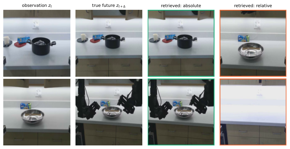
The prediction horizon is four seconds. Commands are absolute targets or the same targets offset by the current state; both presentations use the same frozen visual representation. A teacher trained only on the absolute convention is evaluated under both. The example retrievals show mismatches from other episodes rather than merely adjacent, visually similar frames.
Equation
A certified special case of covariate shift.
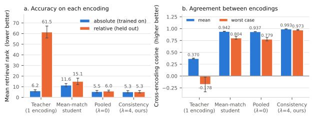
Changing the command encoding is a distribution shift, even when the underlying motion is unchanged. Mean retrieval rank rises from 6.19 to 61.5 on ALOHA cabinet, 3.97 to 53.3 on ALOHA coffee, and 66.2 to 169.8 on PushT, out of 384 candidates. PushT’s mean cross-encoding cosine is 0.067, with an observed minimum of −0.377.
| Retrieval rank | ||||||
|---|---|---|---|---|---|---|
| Dataset | Morphology | Canon. | Held out | Collapse | mean | worst |
| aloha_mobile_cabinet | 14-D bimanual, 50 fps | 6.19 | 61.5 | 0.370 | ||
| aloha_static_coffee | 14-D bimanual, new task | 3.97 | 53.3 | 0.371 | ||
| pusht | 2-D planar pusher, 10 fps | 66.2 | 169.8 | 0.067 | ||
The failure is a control failure.
For each query, the model ranks 32 recorded candidate action windows by how well their predicted future matches the goal. ALOHA cabinet’s top-choice accuracy drops from 53.1% to 15.4% after changing notation. This is an offline action-selection proxy, not measured success from executing commands on a robot.
| Retrieval rank | Agreement | Action selection | ||||
| Canon. | Held out | mean | worst | Canon. | Held out | |
| Teacher | 6.19 | 61.5 | 0.370 | — | ||
| Orbit-mean student | 11.55 | 15.1 | 0.942 | 0.804 | — | — |
| 5.46 | 5.98 | 0.937 | 0.779 | |||
| 5.51 | 5.58 | 0.981 | 0.939 | |||
| 5.25 | 5.31 | 0.993 | 0.973 | |||
| 5.17 | 5.19 | 0.999 | 0.995 | |||
Repair, and what each part of it buys.
Pooled training alone improves held-out-encoding rank from 61.5 to 5.98 and action selection from 15.4% to 40.1%. With penalty weight 16, these become 5.19 and 41.1%; the one-point action-selection gain is smaller than the reported four-point seed variation. The main benefit is observed minimum agreement, 0.779 to 0.995, at a cost in canonical action selection from 44.3% to 41.1%. This minimum summarizes the evaluation set rather than guaranteeing behavior on future inputs.
The mean is stable over a horizon; the worst case is not.
Latent rollouts feed predictions back while supplying true state and action windows at every hop. Prediction quality against the true future decays, so agreeing rollouts can still be wrong. On ALOHA cabinet, the final observed minimum cosine is 0.242 for the teacher, 0.896 for pooled training, and 0.997 with the penalty. PushT remains harder: Table 3 reports final mean/minimum agreement of 0.677/−0.348 for pooling and 0.872/0.139 with the penalty. These are not closed-loop control results.
| Teacher | ||||||
| Dataset | mean | worst | mean | worst | mean | worst |
| ALOHA cabinet | 0.805 | 0.242 | 0.988 | 0.896 | 1.000 | 0.997 |
| ALOHA coffee | 0.898 | 0.614 | 0.991 | 0.955 | 1.000 | 0.998 |
| PushT | 0.178 | 0.677 | 0.872 | 0.139 | ||
On the value of finding the axis.
Exposure to both encodings works only after identifying which transformations are worth treating as equivalent. Pooling inputs that remove predictive information could purchase consistency by sacrificing accuracy.
Where repair is not free.
PushT’s repair improves the unseen-encoding retrieval rank from 169.8 to 85.7 but worsens the canonical rank from 66.2 to 79.2. The accuracy cost makes the intervention dataset dependent.
5.2 The defect is flat in n over the range we can sweep
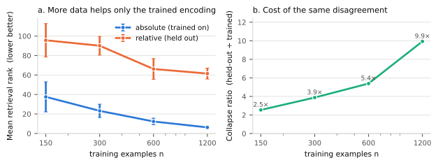
Increasing cached training examples from 150 to 1,200 improves canonical retrieval while cross-encoding cosine stays near 0.34–0.37. The collapse ratio therefore grows from 2.5 to 9.9 without showing growing disagreement itself. Larger and longer-trained models also overfit the fixed data, so those sweeps do not independently establish a clean capacity-scaling result.
Locating I ( Y ; G ∣ Z ) .
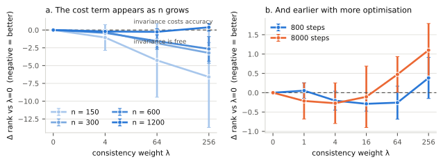
Strong penalties help more with scarce data and can become costly as canonical prediction improves. At weight 256, the rank difference relative to pooling changes from −6.59 with 150 examples to +0.38 with 1,200. The reported practical weights are 4–16.
5.3 Why this axis is the hard case
Some representations remove a transformation before it reaches the predictor: angle features using sine/cosine erase full-turn changes, and excluding absolute time erases time-origin shifts. A molecular example likewise shows that representation choice changes the outcome of attempted invariance repair. A known action convention could also be explicitly normalized in a robot pipeline; this paper studies predictors exposed to both conventions without such a canonicalization step.
6 Discussion
The discussion relates the encoding audit to invariant learning, architectural symmetry, and the limits of the small offline study.
Discovering rather than assuming invariance.
Invariant-risk and causal-invariance methods infer stable prediction across environments. This work instead begins with a proposed transformation and asks whether agreement under it is justified. Automatically proposing useful transformations remains future work. [1] [2]
Relation to prior work.
Architectural equivariance and data augmentation already offer ways to enforce known symmetries. The paper’s focus is diagnosing an overlooked input convention and separating the effects of pooled training from a consistency penalty. [11] [12] [13] [14]
Where repair is unavailable.
The implemented loss enumerates a small set of presentations. Exact enumeration becomes impractical for large permutation groups or continuous transformations. This limits this implementation, rather than proving that sampling or structural alternatives can never help.
Limitations.
Evidence comes from a small MLP, frozen embeddings, three seeds, and offline proxies. Ridge-regression probes may miss nonlinear relationships, and cannot establish all relevant equivalences. Agreement is distinct from predictive correctness; no deployed robot safety or closed-loop task success is established.
Conclusion.
Audit action conventions before trusting latent predictions across interfaces. On the studied datasets, exposure to both representations recovers much of the average performance, while consistency regularization chiefly improves agreement in the observed tail.
Reproducibility statement
The authors describe a Mezzanine repository with cached latents, configurations, seeds, and stored results. Three-seed variation is reported; CPU/GPU retrieval ranks can differ by 2–4% because of floating-point ordering even when dispersion is stable.
Ethics statement
The study reuses public robot-learning data without new collection or human-subject experiments. Its diagnostic is intended for evaluation before control deployment; the measured accuracy–agreement trade-off requires application-specific assessment.
Appendix A Experimental detail
These details specify the datasets, frozen features, predictor, repair loss, and evaluation protocol.
Datasets.
ALOHA cabinet uses 85 episodes, ALOHA coffee 50, and PushT 206, with episode-disjoint splits. The horizon is 200 frames at 50 frames per second for ALOHA and 40 frames at 10 frames per second for PushT. The complete dataset table is preserved.
| Dataset | Camera | Episodes | Frames | fps | (steps) | train/test eps. |
|---|---|---|---|---|---|---|
| aloha_mobile_cabinet | cam_high | 85 | 127,500 | 50 | 200 | 68 / 17 |
| aloha_static_coffee | cam_high | 50 | 55,000 | 50 | 200 | 40 / 10 |
| pusht | image | 206 | 25,650 | 10 | 40 | 165 / 41 |
Encoder.
A frozen I-JEPA ViT-H/14 encodes 224-pixel frames. Features concatenate patch-token means and standard deviations from the fourth-from-last block. No gradient updates the encoder; cached features are tied to the model and preprocessing configuration. [3]
Predictor.
A two-layer MLP of hidden width 1,024 predicts a normalized future embedding from the current latent and 16 sampled action points. Training uses 800 InfoNCE steps, 1,200 examples, and training-only centering statistics; evaluation uses 384 examples.
Repair.
Repair keeps the same training duration while varying the cosine-disagreement weight over 0, 1, 4, and 16. Weight zero retains both action encodings and removes only the consistency term.
Metrics.
Retrieval rank is lower when prediction better identifies the true future among 384 latents. Agreement compares two encodings’ predictions; it does not compare either prediction with truth. Action selection chooses among 32 windows, with chance probability 1/32.
Seeds and hardware.
Seeds 0, 1, and 2 control sampling, initialization, and batching. Runs use one RTX 5090; reported short sweep times exclude the initial video-decoding and feature-caching work.
What is not controlled.
Three seeds give limited uncertainty estimates. Capacity and optimization sweeps use the same 1,200 examples, so worse canonical performance confounds conclusions about scaling.
Appendix B Action ablations are not orbit-constancy tests
Shuffling actions between examples tests whether a model uses its action input. It changes the commanded trajectory and therefore cannot establish invariance to an equivalent notation. The supplementary action-ablation results should be read separately from the main encoding experiment.
Repair beyond robotics.
In a node-permutation example, target-based pooled training reduces dispersion more than fitting averaged teacher outputs, with slightly lower test error. Periodic integration changes little because its features already remove the relevant nuisance.
Appendix C Rollout divergence, per hop
The per-hop table retains complete rollout trajectories. Chains start earlier in episodes to leave sufficient runway, so their absolute agreement should not be compared directly with the single-step sample. ALOHA uses three hops and PushT two.
| Mean | Worst-case | ||||||
|---|---|---|---|---|---|---|---|
| Dataset | Model | hop 1 | hop 2 | hop 3 | hop 1 | hop 2 | hop 3 |
| ALOHA | Teacher | 0.836 | 0.803 | 0.805 | 0.515 | 0.350 | 0.242 |
| cabinet | 0.992 | 0.990 | 0.988 | 0.972 | 0.951 | 0.896 | |
| 1.000 | 1.000 | 1.000 | 1.000 | 0.999 | 0.997 | ||
| ALOHA | Teacher | 0.916 | 0.889 | 0.898 | 0.707 | 0.676 | 0.614 |
| coffee | 0.995 | 0.993 | 0.991 | 0.987 | 0.973 | 0.955 | |
| 1.000 | 1.000 | 1.000 | 1.000 | 0.999 | 0.998 | ||
| Teacher | 0.246 | 0.178 | — | — | |||
| PushT | 0.633 | 0.677 | — | — | |||
| 0.946 | 0.872 | — | 0.666 | 0.139 | — | ||
Appendix D Additional results
Additional tables and figures compare scaling, penalty strength, and transformations whose information is already removed by the representation.
D.1 Symmetry breaking along data, optimization and capacity
The table contrasts larger datasets, longer optimization, and wider predictors. The latter two also worsen canonical performance on this small dataset, limiting their interpretation as evidence about model scale.
| Axis | Varied | From | To |
|---|---|---|---|
| Data | collapse | ||
| Optimization | steps | ||
| Capacity | hidden | ||
D.2 When the orbit is too large to enumerate
Two action conventions can be enumerated cheaply. The following examples explain why that convenience does not extend automatically to large or continuous transformation families.
Discrete orbits grow factorially.
There are N! permutations of N interchangeable items. Independent Monte Carlo averaging reduces standard deviation only as the inverse square root of sample count, so demanding near-exact agreement can be expensive.
Continuous orbits are not finite sums at all.
A continuous transformation family requires integration rather than a finite exact sum. Finite sampling can approximate it, but does not enumerate the full orbit.
Where that leaves robot dynamics.
Small convention sets suit the implemented pooled loss. Larger symmetries motivate encoders or architectures that remove or respect the transformation directly.
D.3 True symmetry breaking at finite n
For a synthetic permutation-invariant classification target, invariant models retain high accuracy while unrestricted models show finite-data dispersion. More data reduces that dispersion; increasing dimension makes the unrestricted task harder. This controlled example differs from the one-convention robot training setup.
| Acc (unconstr.) | Acc (invariant) | Orbit disp. | |||
|---|---|---|---|---|---|
| 8 | 1,000 | 0.858 | 0.979 | 0.141 | |
| 8 | 10,000 | 0.942 | 0.993 | 0.059 | |
| 8 | 100,000 | 0.968 | 0.995 | 0.024 | |
| 16 | 1,000 | 0.756 | 0.974 | 0.229 | |
| 16 | 10,000 | 0.828 | 0.991 | 0.163 | |
| 16 | 100,000 | 0.918 | 0.994 | 0.062 | |
| 32 | 1,000 | 0.708 | 0.978 | 0.277 | |
| 32 | 10,000 | 0.757 | 0.991 | 0.224 | |
| 32 | 100,000 | 0.810 | 0.993 | 0.151 |
D.4 Collapse ratio against training-set size
The data-size figure separates canonical and alternative-encoding retrieval. Their ratio worsens because the trained convention improves, while the measured directional disagreement stays approximately flat.
D.5 Cost of orbit-constancy versus λ
The penalty sweep plots rank changes relative to pooled training. Negative values indicate improvement; large penalties become less favorable with more data or optimization.
D.6 Admissibility certificates on four numerical axes
Angle wrapping and time-origin shifts show almost no dispersion because their representations already omit the nuisance. Circular shifts and node permutations show measurable differences that the tested repair reduces.
| Axis | Family | Teacher dispersion | Reduction | Certificate |
|---|---|---|---|---|
| Angle wrap (Kepler) | gauge | — | bijective | |
| Time origin (Lorenz) | gauge | — | bijective | |
| Circular shift | gauge | quotient | ||
| Node permutation (Ax=b) | exchangeability | quotient |
Appendix E Description-length account of the incentive
The appendix decomposes a description-length objective into model-description cost and best-achievable empirical prediction loss. It distinguishes empirical predictive benefit from approximation error and population information; these algebraic identities do not themselves demonstrate how a neural optimizer will behave. [15] [16]
Three regimes, not one conclusion.
Three cases matter: the changed coordinate carries target information; the target is truly invariant but finite data or model misspecification create gaps; or training never varies the coordinate at all. The robot convention experiment primarily concerns the third case. The original definitions and formal statements remain available in the source paper.
Equations
E.1 Orbit-constancy
Under a genuinely invariant target distribution and a strictly proper scoring rule, the Bayes-optimal prediction shares that invariance. Independent orbit samples reduce the variance of their mean by the sample count. Both statements depend on their stated distributional and sampling assumptions.
Appendix F Proof of Theorem 2
The proof defines a quotient over presentations identified as equivalent and derives a lower bound from the information that quotient discards.
Step 1: orbit-constant predictors are exactly the Q -measurable ones.
An orbit-constant prediction depends only on the quotient class Q. Its optimal log loss is consequently the conditional entropy of the target given Q.
Equation
Step 2: Q is a coarsening of every view.
Each individual view determines Q, so passing to Q cannot improve the optimal prediction risk over that view.
Equation
Step 3.
Taking the worst individual-view risk and subtracting the best produces the stated lower bound on the cost of forcing agreement.
Equality, and the two certificates.
The authors propose mutual reconstructibility and predictive parity as certificates for zero invariance cost. As qualified in Section 3, these checks alone do not prove target sufficiency for a shared, unlabeled view space; the quotient must also retain the information needed to predict the target.
Beyond log loss.
The coarsening argument extends to strictly proper scoring rules through their generalized Bayes risk. Its lower bound similarly compares the best achievable risks before and after imposing agreement.
Appendix G Direction-valued prediction has no Jensen guarantee
For probability predictions, concavity of the logarithm bounds mixture log loss by the average component loss. For unit-vector predictions, three vectors scoring 1, −0.9, and −0.9 against the target can have a normalized mean scoring −1. Opposite vectors can cancel entirely. These counterexamples explain why the robot experiment averages losses instead of normalizing averaged outputs.
Equations
Audit and repair.
The retained algorithm first evaluates the proposed equivalence, then measures dispersion and task performance, fits the pooled objective, and checks bootstrap intervals against a tolerance. A favorable finite-data audit supports the tested operating point, without proving universal invariance or future task safety.
Appendix H Supplementary experiments
Supplementary experiments examine periodic integration, node permutation, and molecular representations as contrasting invariance cases.
H.1 Action-conditioned dynamics: robotics and iPhyRE
Supplementary ablations show benefits from action conditioning on ALOHA, LIBERO-10, and iPhyRE, with degradation after cross-example action shuffling. PushT instead has worse mean retrieval rank when actions are added. These experiments test action usefulness, not agreement under equivalent representations.
| Task | rank (no-act) | rank (act) | rank (shuf) | R@10 (no-act) | R@10 (act) | Verdict |
|---|---|---|---|---|---|---|
| ALOHA | 186.2 | 97.7 | 635.8 | 0.068 | 0.124 | make |
| LIBERO-10 | 80.9 | 49.6 | 55.5 | 0.136 | 0.242 | make |
| PushT | 179.9 | 349.9 | 547.7 | 0.079 | 0.093 | break |
| Metric | persist | no action | action | shuf |
|---|---|---|---|---|
| mean rank | 167.5 | 172.6 | 31.3 | 173.9 |
| Recall@10 | 0.203 | 0.185 | 0.471 | 0.124 |
H.2 Molecular dynamics: representation ablation
For Lennard-Jones dynamics, an invariant radial-distribution representation preserves classification accuracy under the tested distillation, roughly 0.894 to 0.893. Flattened coordinates instead fall from 0.856 to 0.456. The result shows the importance of representation and finite approximation in this setup, rather than an impossibility theorem for all symmetry-aware models.