At a glance
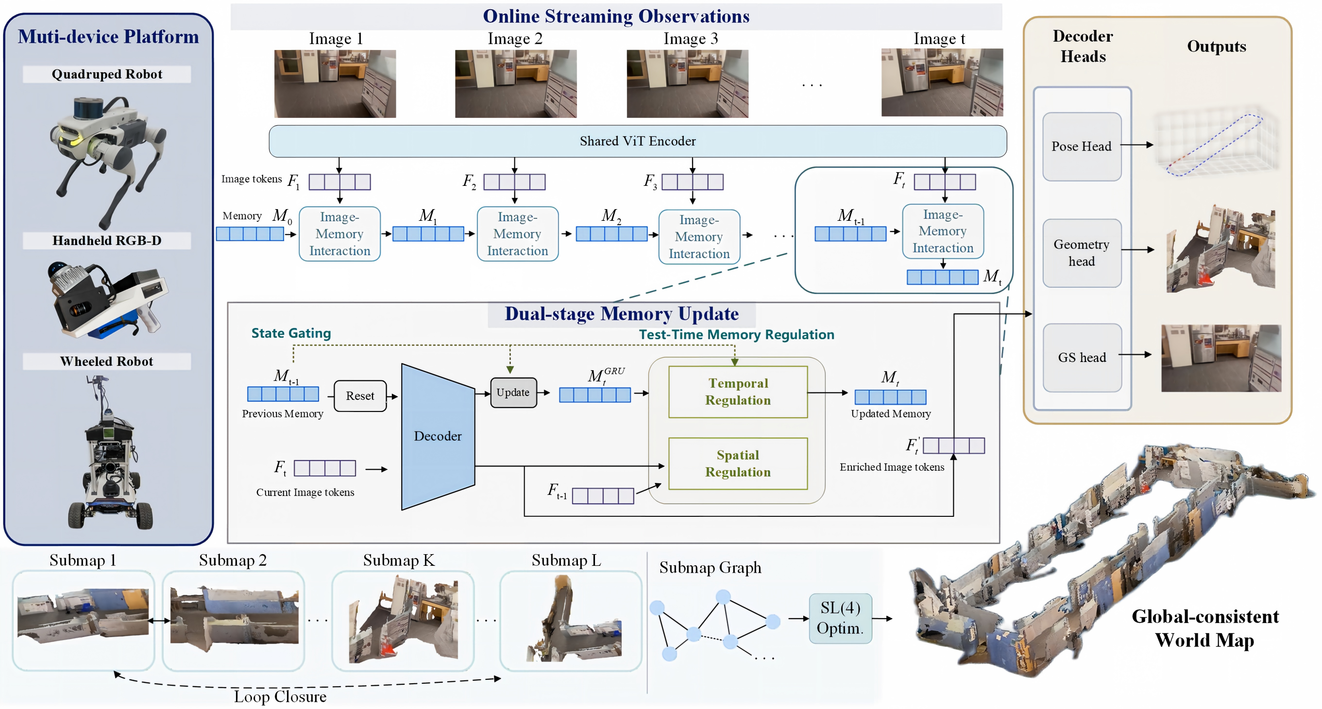
Adaptive World Memory combines recurrent geometric features, observation-dependent update masks, local submaps and global alignment. The same features predict camera poses, pointmaps and renderable Gaussian primitives from streaming monocular RGB images.
Public benchmarks and selected robot sequences show useful depth, trajectory, reconstruction and rendering results. The tables support task-specific improvements rather than uniform dominance. Constant active-state size should also be distinguished from the storage required by a growing collection of persistent submaps.
This edition follows the complete 19-page first arXiv version, including all references. The paper links a proposed code and dataset repository; its text describes those resources as a forthcoming release.
I Introduction
Pairwise and full-attention geometric models have limited context or increasing long-sequence cost. Recurrent models retain history, but unreliable observations can corrupt their state. A useful robotic map also needs global correction and a representation that can be rendered.
The paper combines learned reset/update gates with a test-time temporal–spatial mask. Local submaps limit recurrent propagation; loop constraints and projective submap optimization correct global drift. A Gaussian head adds visual rendering to the shared pose/pointmap representation.
The evaluations test mapping and localization across several platforms. Navigation, manipulation and downstream decision-making remain proposed uses rather than demonstrated policy improvements.
II Related Works
The related work connects scene representations, feed-forward geometric foundation models, streaming memory and classical global-consistency methods.
II-A Scene Representations for Mapping and Localization
Sparse landmarks support localization but limited surface detail. Dense point clouds and surfels capture more geometry, while radiance fields and Gaussian splats support rendering. Learned geometric priors can reduce scene-specific initialization work.
The proposed system combines these goals: explicit geometry and renderable primitives are predicted from a shared learned memory, with additional tracking and global optimization.
II-B 3D Foundation models
DUSt3R and MASt3R predict pointmaps and correspondences; VGGT and related models extend geometric reasoning across multiple views. Full-sequence attention and short-window processing face different memory/context limits.
The paper targets persistent streaming use, rather than showing that every feed-forward alternative is inferior on short sequences.
II-C Online and Memory-based 3D Foundation Models
Streaming transformers, recurrent state tokens, explicit spatial memory and test-time adaptation offer different ways to reuse history. This work combines recurrent gating with a forward-computed online regulation mask and submap management.
The method equations describe feature/state regulation at inference. They do not specify gradient-based online weight training for these masks, despite broader discussion of test-time-training methods.
II-D Scalable SLAM Optimization and Global Consistency
Keyframes, local tracking, loop closure and graph optimization remain useful alongside learned geometry. Independent submaps localize state updates and provide units for global correction.
The proposed projective backend is more flexible than rigid or similarity alignment, which also means that global consistency is not synonymous with a strictly rigid metric reconstruction.
III Method
The method links a dual-stage local memory to pose/pointmap heads, a Gaussian head, local tracking and a loop-aware submap graph. All 38 numbered equations are retained.
III-A Framework Overview
Incoming monocular RGB frames are encoded into geometric tokens. Memory-enhanced tokens predict self-coordinate pointmaps, active-submap-coordinate pointmaps, confidence and camera pose. No depth measurement or prebuilt map is required at inference.
Renderable Gaussians are inserted into local maps. Tracking refines the predicted pose, while occasional submap creation and loop closure trigger global alignment. “World-coordinate” pointmaps in the front end refer to the active submap, rather than the final globally aligned frame.
III-B Dual-Stage Adaptive World Memory
The active submap maintains N latent memory tokens. A learned gated update produces a candidate; temporal state change and observation/attention cues then regulate how much of that candidate enters memory.
III-B 1 Gated Recurrent Spatial State
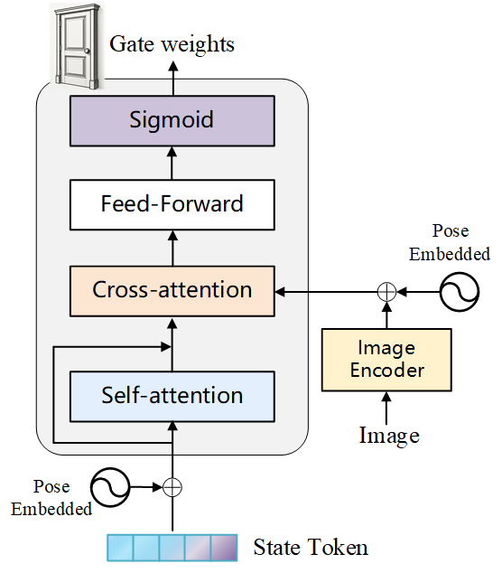
Transformer reset and update gates combine the previous state with current visual features. Reset memory enters a decoder with image and pose tokens; cross-attention exchanges current observations and historical context. The update gate blends the candidate with the preceding state.
The second stage adds observation-dependent regulation to these learned gates. Figure 2 retains the complete gate architecture.
Equations 1–4
| (1) |
| (2) |
| (3) |
| (4) |
III-B 2 Test-Time Temporal–Spatial Memory Regulation
Temporal regulation measures each candidate token’s change, normalizes by the mean change and applies a sigmoid threshold. Spatial regulation combines inter-frame cosine dissimilarity with averaged cross-attention, then applies a sigmoid to the largest weighted change. Their product controls the final update.
These are feature-based heuristics for useful change, rather than calibrated reliability estimates. Equation 10’s nonnegative input means its spatial sigmoid is at least one half, including unchanged features; it is not a hard zero-update mask. The first frame and sequence resets bypass regulation.
Equations 5–11
| (5) |
| (6) |
| (7) |
| (8) |
| (9) |
| (10) | ||||
| (11) |
III-B 3 Dual-Stage Memory Update
The final state blends the gated candidate with the old memory using the temporal–spatial mask. The updated image/pose features feed the geometric heads.
This construction can attenuate updates; the equations do not guarantee that every unreliable observation is rejected or that memory contamination is impossible.
Equations 12–15
| (12) |
| (13) |
| (14) |
| (15) |
III-C Feed-forward Gaussian World Representation
Gaussian centers are anchored to active-submap pointmaps. A dense geometry decoder and shallow image encoder predict opacity, rotation, scale and appearance. Detached pointmap confidence controls insertion, without receiving rendering-loss gradients through that confidence score.
Predicted intrinsics are adjusted once for inference-to-renderer resizing and cropping. Differentiable splatting then renders the local map using the predicted pose. The complete covariance, confidence, insertion and intrinsic-transform equations are preserved.
This is feed-forward primitive prediction within a system that also performs tracking/refinement; it should not be read as removal of every online optimization step.
Equations 16–23
| (16) |
| (17) |
| (18) |
| (19) |
| (20) |
| (21) |
| (22) | ||||||
| (23) |
III-D Progressive Mapping and Tracking
Foundation-model pose estimates initialize confidence-weighted alignment against the active local map. The refined pose supports insertion of reliable pointmap and Gaussian predictions.
III-D 1 Submap-Aware Local Mapping and Tracking
Each submap stores memory, keyframes, poses, pointmaps, confidence and Gaussians. Overlap with the latest keyframe controls insertion; overlap with the anchor controls new-submap creation. New memory is initialized from the image and a learned empty prior.
Inactive submaps remain persistent. Fixed-size active memory bounds one recurrent state, while total map storage can grow with submaps, retained observations and inserted primitives. No general constant-storage guarantee follows from this organization.
Equations 24–26
| (24) |
| (25) |
| (26) |
III-D 2 Loop Closure and SL(4)-Based Global Optimization
Sequential and loop edges connect overlapping submaps. Their 4×4 unit-determinant homographies permit scale, shear, stretch and projective correction beyond rigid or similarity transforms.
This extra flexibility can absorb residual reconstruction distortion. It also requires care when interpreting a globally transformed map as metric geometry.
Equation 27
| (27) |
Relative Submap Alignment.
Dense cross-submap point correspondences estimate a relative homography with a RANSAC solver. Shared observations supply adjacent constraints; retrieved frames are reconstructed in both local systems for loop constraints.
Equation 28 normalizes by the determinant’s fourth root. Degenerate and negative-determinant cases are not discussed, so the displayed formula alone is not a complete robust-solver specification.
Equation 28
| (28) |
Loop Closure Detection.
UniPR-3D descriptors retrieve non-adjacent historical keyframes. Descriptor similarity, inlier count and geometric residual thresholds jointly verify candidate loops before accepting their constraints.
The paper describes these tests but does not provide all threshold values or a separate loop precision/recall evaluation.
Equation 29
| (29) |
Global Optimization on the SL(4) Manifold.
A factor graph minimizes Lie-algebra residuals on SL(4), anchoring the first submap to fix gauge. Tangent-space updates refine each transformation.
Centers are transformed projectively; Gaussian covariances use the projection’s local Jacobian. This is a local affine approximation: a general projective warp does not exactly preserve a Gaussian distribution. The document gives limited detail on converting transformed camera poses back to rigid pose parameters.
Equations 30–31
| (30) |
| (31) |
III-E Training Objectives
Training combines geometric, pose, rendering and Gaussian regularization losses. Rendering supervision uses images rather than ground-truth Gaussian primitives. Online tracking/refinement is an additional part of inference.
Pointmap regression loss.
Confidence-weighted point regression balances geometric error against a log-confidence penalty. Both self-coordinate and active-submap pointmaps are supervised. Scale normalization is shared with pose translation; metric training data use matching normalization factors.
Equations 32–33
| (32) |
| (33) |
Pose loss.
Pose supervision penalizes quaternion and normalized translation discrepancies. The displayed objective is preserved exactly; the paper does not detail quaternion sign handling in this section.
Equation 34
| (34) |
Gaussian rendering loss.
Image L 1, structural similarity and perceptual losses supervise rendered Gaussians using predicted poses and resize/crop-adjusted predicted intrinsics. No direct Gaussian-parameter labels are needed.
Equation 35
| (35) |
Gaussian regularization.
Regularization penalizes opacity magnitude and scale norms outside a selected interval. Detached geometric confidence remains an insertion criterion rather than a separate trainable rendering-confidence variable.
Equations 36–37
| (36) |
| (37) |
Overall training objective.
The total objective weights geometry, pose, image rendering and Gaussian regularization. The original equation retains every term; the text does not supply a complete numerical loss-weight specification.
Equation 38
| (38) |
Curriculum training.
The curriculum starts with short sequences and mostly frozen backbone layers, then unfreezes the decoder, and finally extends sequence length while fine-tuning the model.
Training datasets, stage durations, exact sequence lengths, input resolution and several thresholds are not fully specified in the implementation description.
IV Experiments
Evaluation covers depth, camera trajectory, dense reconstruction and rendering on public datasets plus selected multi-platform recordings. Comparisons have different calibration, alignment and sequence-access assumptions.
IV-A Experiments Setup
The following sections define datasets, reference measurements, metrics and compute. All original result tables remain complete, including failures and excluded categories.
IV-A 1 Test Datasets.
Public benchmarks include Sintel, Bonn, KITTI, Replica, 7-Scenes, TUM RGB-D, ScanNet, NRGBD and BundleFusion. Apartment and robot recordings test longer sequences and global consistency.
Per-sequence scale-aligned depth, metric depth, aligned reconstruction and calibrated/uncalibrated pose results answer different questions and should be compared within their stated protocols.
IV-A 2 Self-Collected Multi-Platform Dataset.
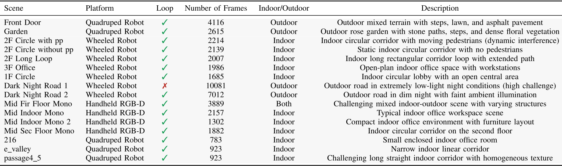
The dataset table lists 16 sequences from handheld, wheeled and quadruped platforms in Singapore and Shanghai, including corridors, offices, vegetation and dark roads. Five representative sequences receive quantitative trajectory comparisons later.
FAST-LIO supplies LiDAR-based reference trajectories, synchronized and calibrated into the camera frame. LiDAR is used for evaluation references; the proposed inference input remains RGB. These references are estimates rather than an independent motion-capture system.
Accessible table and source citation links
| Scene | Platform | Loop | Number of Frames | Indoor/Outdoor | Description |
|---|---|---|---|---|---|
| Front Door | Quadruped Robot | ✓ | 4116 | Outdoor | Outdoor mixed terrain with steps, lawn, and asphalt pavement |
| Garden | Quadruped Robot | ✓ | 2615 | Outdoor | Outdoor rose garden with stone paths, steps, and dense floral vegetation |
| 2F Circle with pp | Wheeled Robot | ✓ | 2214 | Indoor | Indoor circular corridor with moving pedestrians (dynamic interference) |
| 2F Circle without pp | Wheeled Robot | ✓ | 2139 | Indoor | Static indoor circular corridor with no pedestrians |
| 2F Long Loop | Wheeled Robot | ✓ | 2007 | Indoor | Indoor long rectangular corridor loop with extended path |
| 3F Office | Wheeled Robot | ✓ | 1986 | Indoor | Open-plan indoor office space with workstations |
| 1F Circle | Wheeled Robot | ✓ | 1685 | Indoor | Indoor circular lobby with an open central area |
| Dark Night Road 1 | Wheeled Robot | ✗ | 10081 | Outdoor | Outdoor road in extremely low-light night conditions (high challenge) |
| Dark Night Road 2 | Wheeled Robot | ✓ | 7012 | Outdoor | Outdoor road in dim night with faint ambient illumination |
| Mid Fir Floor Mono | Handheld RGB-D | ✓ | 3889 | Both | Challenging mixed indoor-outdoor scene with varying structures |
| Mid Indoor Mono | Handheld RGB-D | ✓ | 2157 | Indoor | Typical indoor office workspace scene |
| Mid Indoor Mono 2 | Handheld RGB-D | ✓ | 1302 | Indoor | Compact indoor office environment with furniture layout |
| Mid Sec Floor Mono | Handheld RGB-D | ✓ | 1882 | Indoor | Indoor circular corridor on the second floor |
| 216 | Quadruped Robot | ✓ | 783 | Indoor | Small enclosed indoor office room |
| e_valley | Quadruped Robot | ✓ | 923 | Indoor | Narrow indoor linear corridor |
| passage4_5 | Quadruped Robot | ✓ | 923 | Indoor | Challenging long straight indoor corridor with homogeneous texture |
IV-A 3 Evaluation Metrics.
Depth uses absolute relative error and a 1.25-ratio threshold. Trajectories use absolute error and adjacent-frame translation/rotation errors. Reconstruction uses untruncated nearest-neighbor distances in both directions after global similarity alignment and ICP.
That reconstruction alignment can correct global scale and pose discrepancies, so those distances alone do not establish raw metric accuracy. Rendering reports PSNR, SSIM and LPIPS on held-out views; efficiency concerns throughput and GPU memory.
IV-A 4 Implementation Details.
Training uses eight 80 GB A100 GPUs; inference uses one RTX 4090. Online input is sequential without future frames, and new submaps or detected loops trigger global optimization.
The text says input resolution is fixed but does not give its numerical value here. A complete reproduction would also need missing training and threshold details.
IV-B Video Depth Estimation
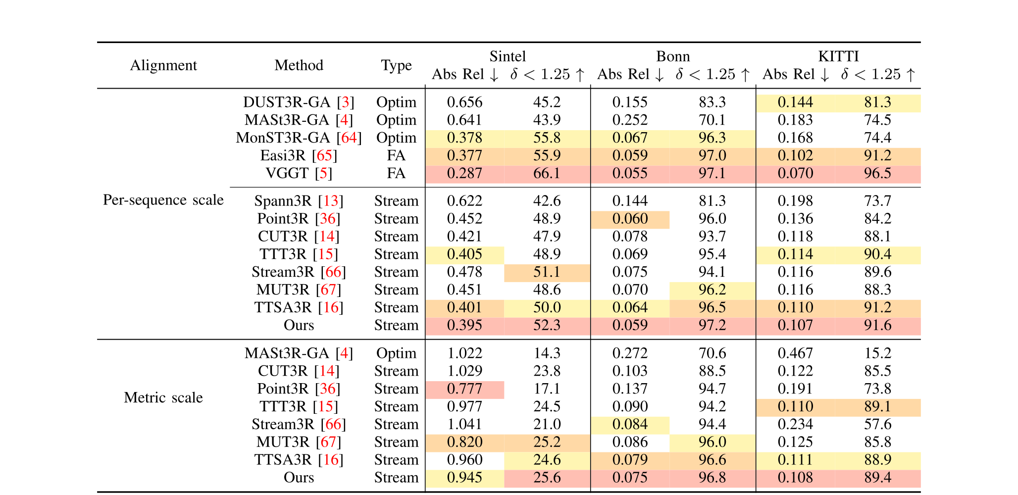
Table II shows strong streaming depth results, but not universal best values. Under metric scale on Sintel, Point3R has lower absolute relative error than this method:0.777 versus 0.945. Full-attention VGGT is stronger on several scale-aligned short-sequence metrics.
On Replica, the reported metric-scale average error is 0.0610, close to TTT3R’s 0.0612. Stream3R is substantially stronger under per-sequence alignment, with 0.0311 versus 0.0494. Its metric absolute-error row contains values even though the caption says metric evaluation is unsupported; its metric threshold entries are missing. All original entries are retained.
Accessible table and source citation links
| Alignment | Method | Type | Sintel | Bonn | KITTI | |||
|---|---|---|---|---|---|---|---|---|
| Abs Rel | Abs Rel | Abs Rel | ||||||
| Per-sequence scale | DUST3R-GA [3] | Optim | 0.656 | 45.2 | 0.155 | 83.3 | 0.144 | 81.3 |
| MASt3R-GA [4] | Optim | 0.641 | 43.9 | 0.252 | 70.1 | 0.183 | 74.5 | |
| MonST3R-GA [64] | Optim | 0.378 | 55.8 | 0.067 | 96.3 | 0.168 | 74.4 | |
| Easi3R [65] | FA | 0.377 | 55.9 | 0.059 | 97.0 | 0.102 | 91.2 | |
| VGGT [5] | FA | 0.287 | 66.1 | 0.055 | 97.1 | 0.070 | 96.5 | |
| Spann3R [13] | Stream | 0.622 | 42.6 | 0.144 | 81.3 | 0.198 | 73.7 | |
| Point3R [36] | Stream | 0.452 | 48.9 | 0.060 | 96.0 | 0.136 | 84.2 | |
| CUT3R [14] | Stream | 0.421 | 47.9 | 0.078 | 93.7 | 0.118 | 88.1 | |
| TTT3R [15] | Stream | 0.405 | 48.9 | 0.069 | 95.4 | 0.114 | 90.4 | |
| Stream3R [66] | Stream | 0.478 | 51.1 | 0.075 | 94.1 | 0.116 | 89.6 | |
| MUT3R [67] | Stream | 0.451 | 48.6 | 0.070 | 96.2 | 0.116 | 88.3 | |
| TTSA3R [16] | Stream | 0.401 | 50.0 | 0.064 | 96.5 | 0.110 | 91.2 | |
| Ours | Stream | 0.395 | 52.3 | 0.059 | 97.2 | 0.107 | 91.6 | |
| Metric scale | MASt3R-GA [4] | Optim | 1.022 | 14.3 | 0.272 | 70.6 | 0.467 | 15.2 |
| CUT3R [14] | Stream | 1.029 | 23.8 | 0.103 | 88.5 | 0.122 | 85.5 | |
| Point3R [36] | Stream | 0.777 | 17.1 | 0.137 | 94.7 | 0.191 | 73.8 | |
| TTT3R [15] | Stream | 0.977 | 24.5 | 0.090 | 94.2 | 0.110 | 89.1 | |
| Stream3R [66] | Stream | 1.041 | 21.0 | 0.084 | 94.4 | 0.234 | 57.6 | |
| MUT3R [67] | Stream | 0.820 | 25.2 | 0.086 | 96.0 | 0.125 | 85.8 | |
| TTSA3R [16] | Stream | 0.960 | 24.6 | 0.079 | 96.6 | 0.111 | 88.9 | |
| Ours | Stream | 0.945 | 25.6 | 0.075 | 96.8 | 0.108 | 89.4 | |
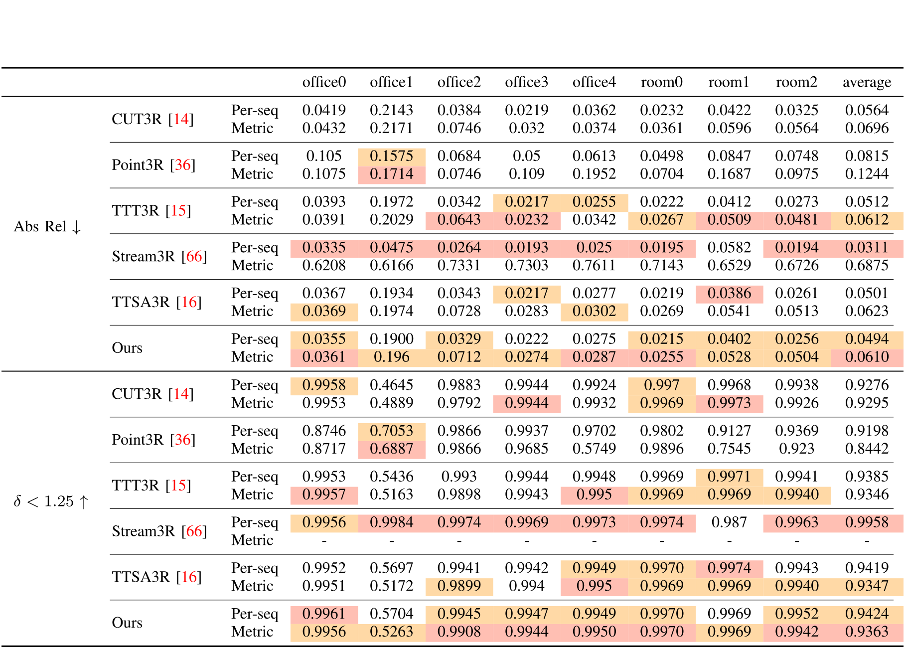
Accessible table and source citation links
| office0 | office1 | office2 | office3 | office4 | room0 | room1 | room2 | average | |||
|---|---|---|---|---|---|---|---|---|---|---|---|
| Abs Rel | CUT3R[14] | Per-seq | 0.0419 | 0.2143 | 0.0384 | 0.0219 | 0.0362 | 0.0232 | 0.0422 | 0.0325 | 0.0564 |
| Metric | 0.0432 | 0.2171 | 0.0746 | 0.032 | 0.0374 | 0.0361 | 0.0596 | 0.0564 | 0.0696 | ||
| Point3R[36] | Per-seq | 0.105 | 0.1575 | 0.0684 | 0.05 | 0.0613 | 0.0498 | 0.0847 | 0.0748 | 0.0815 | |
| Metric | 0.1075 | 0.1714 | 0.0746 | 0.109 | 0.1952 | 0.0704 | 0.1687 | 0.0975 | 0.1244 | ||
| TTT3R[15] | Per-seq | 0.0393 | 0.1972 | 0.0342 | 0.0217 | 0.0255 | 0.0222 | 0.0412 | 0.0273 | 0.0512 | |
| Metric | 0.0391 | 0.2029 | 0.0643 | 0.0232 | 0.0342 | 0.0267 | 0.0509 | 0.0481 | 0.0612 | ||
| Stream3R[66] | Per-seq | 0.0335 | 0.0475 | 0.0264 | 0.0193 | 0.025 | 0.0195 | 0.0582 | 0.0194 | 0.0311 | |
| Metric | 0.6208 | 0.6166 | 0.7331 | 0.7303 | 0.7611 | 0.7143 | 0.6529 | 0.6726 | 0.6875 | ||
| TTSA3R[16] | Per-seq | 0.0367 | 0.1934 | 0.0343 | 0.0217 | 0.0277 | 0.0219 | 0.0386 | 0.0261 | 0.0501 | |
| Metric | 0.0369 | 0.1974 | 0.0728 | 0.0283 | 0.0302 | 0.0269 | 0.0541 | 0.0513 | 0.0623 | ||
| Ours | Per-seq | 0.0355 | 0.1900 | 0.0329 | 0.0222 | 0.0275 | 0.0215 | 0.0402 | 0.0256 | 0.0494 | |
| Metric | 0.0361 | 0.196 | 0.0712 | 0.0274 | 0.0287 | 0.0255 | 0.0528 | 0.0504 | 0.0610 | ||
| CUT3R[14] | Per-seq | 0.9958 | 0.4645 | 0.9883 | 0.9944 | 0.9924 | 0.997 | 0.9968 | 0.9938 | 0.9276 | |
| Metric | 0.9953 | 0.4889 | 0.9792 | 0.9944 | 0.9932 | 0.9969 | 0.9973 | 0.9926 | 0.9295 | ||
| Point3R[36] | Per-seq | 0.8746 | 0.7053 | 0.9866 | 0.9937 | 0.9702 | 0.9802 | 0.9127 | 0.9369 | 0.9198 | |
| Metric | 0.8717 | 0.6887 | 0.9866 | 0.9685 | 0.5749 | 0.9896 | 0.7545 | 0.923 | 0.8442 | ||
| TTT3R[15] | Per-seq | 0.9953 | 0.5436 | 0.993 | 0.9944 | 0.9948 | 0.9969 | 0.9971 | 0.9941 | 0.9385 | |
| Metric | 0.9957 | 0.5163 | 0.9898 | 0.9943 | 0.995 | 0.9969 | 0.9969 | 0.9940 | 0.9346 | ||
| Stream3R[66] | Per-seq | 0.9956 | 0.9984 | 0.9974 | 0.9969 | 0.9973 | 0.9974 | 0.987 | 0.9963 | 0.9958 | |
| Metric | - | - | - | - | - | - | - | - | - | ||
| TTSA3R[16] | Per-seq | 0.9952 | 0.5697 | 0.9941 | 0.9942 | 0.9949 | 0.9970 | 0.9974 | 0.9943 | 0.9419 | |
| Metric | 0.9951 | 0.5172 | 0.9899 | 0.994 | 0.995 | 0.9969 | 0.9969 | 0.9940 | 0.9347 | ||
| Ours | Per-seq | 0.9961 | 0.5704 | 0.9945 | 0.9947 | 0.9949 | 0.9970 | 0.9969 | 0.9952 | 0.9424 | |
| Metric | 0.9956 | 0.5263 | 0.9908 | 0.9944 | 0.9950 | 0.9970 | 0.9969 | 0.9942 | 0.9363 |
IV-C Camera Pose Estimation
The paper reports uncalibrated average trajectory errors of 0.064 m on 7-Scenes and 0.042 m on TUM RGB-D. Some 7-Scenes row averages do not match their seven printed entries: this method’s entries average approximately 0.0783 m, rather than 0.064 m. Reported and recomputed values should not be silently substituted.
Dynamic-scene results are mixed: TTSA3R outperforms this method on all three TUM-dynamics metrics, while the new method improves ScanNet’s listed streaming trajectory errors. On Replica, its 3.05 cm average leads the selected foundation-model comparison; conventional calibrated/uncalibrated SLAM rows have lower errors and are excluded from that ranking.
On KITTI, the best listed learning-based average is obtained only after excluding high-speed sequence 01:44.762 m. Across all sequences, its 53.509 m is slightly worse than DPV-SLAM’s 53.034 m. Classical methods are displayed but excluded from the authors’ ranking.
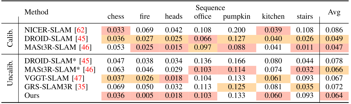
Accessible table and source citation links
| Method | Sequence | Avg | |||||||
|---|---|---|---|---|---|---|---|---|---|
| chess | fire | heads | office | pumpkin | kitchen | stairs | |||
| Calib. | NICER-SLAM [62] | 0.033 | 0.069 | 0.042 | 0.108 | 0.200 | 0.039 | 0.108 | 0.086 |
| DROID-SLAM [45] | 0.036 | 0.027 | 0.025 | 0.066 | 0.127 | 0.040 | 0.026 | 0.049 | |
| MASt3R-SLAM [46] | 0.053 | 0.025 | 0.015 | 0.097 | 0.088 | 0.041 | 0.011 | 0.047 | |
| Uncalib. | DROID-SLAM* [45] | 0.047 | 0.038 | 0.034 | 0.136 | 0.166 | 0.080 | 0.044 | 0.078 |
| MASt3R-SLAM* [46] | 0.063 | 0.046 | 0.029 | 0.103 | 0.114 | 0.074 | 0.032 | 0.066 | |
| VGGT-SLAM [47] | 0.037 | 0.026 | 0.018 | 0.104 | 0.133 | 0.061 | 0.093 | 0.067 | |
| GRS-SLAM3R [35] | 0.069 | 0.050 | 0.032 | 0.113 | 0.125 | 0.081 | 0.035 | 0.072 | |
| Ours | 0.036 | 0.005 | 0.018 | 0.103 | 0.133 | 0.060 | 0.093 | 0.064 | |
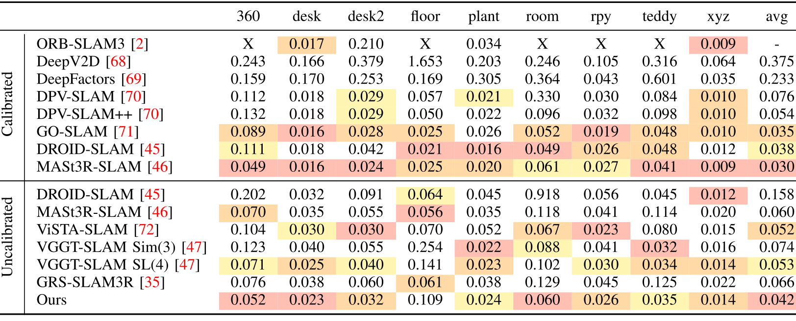
Accessible table and source citation links
| 360 | desk | desk2 | floor | plant | room | rpy | teddy | xyz | avg | ||
| Calibrated | ORB-SLAM3 [2] | X | 0.017 | 0.210 | X | 0.034 | X | X | X | 0.009 | - |
| DeepV2D [68] | 0.243 | 0.166 | 0.379 | 1.653 | 0.203 | 0.246 | 0.105 | 0.316 | 0.064 | 0.375 | |
| DeepFactors [69] | 0.159 | 0.170 | 0.253 | 0.169 | 0.305 | 0.364 | 0.043 | 0.601 | 0.035 | 0.233 | |
| DPV-SLAM [70] | 0.112 | 0.018 | 0.029 | 0.057 | 0.021 | 0.330 | 0.030 | 0.084 | 0.010 | 0.076 | |
| DPV-SLAM++ [70] | 0.132 | 0.018 | 0.029 | 0.050 | 0.022 | 0.096 | 0.032 | 0.098 | 0.010 | 0.054 | |
| GO-SLAM [71] | 0.089 | 0.016 | 0.028 | 0.025 | 0.026 | 0.052 | 0.019 | 0.048 | 0.010 | 0.035 | |
| DROID-SLAM [45] | 0.111 | 0.018 | 0.042 | 0.021 | 0.016 | 0.049 | 0.026 | 0.048 | 0.012 | 0.038 | |
| MASt3R-SLAM [46] | 0.049 | 0.016 | 0.024 | 0.025 | 0.020 | 0.061 | 0.027 | 0.041 | 0.009 | 0.030 | |
| Uncalibrated | DROID-SLAM [45] | 0.202 | 0.032 | 0.091 | 0.064 | 0.045 | 0.918 | 0.056 | 0.045 | 0.012 | 0.158 |
| MASt3R-SLAM [46] | 0.070 | 0.035 | 0.055 | 0.056 | 0.035 | 0.118 | 0.041 | 0.114 | 0.020 | 0.060 | |
| ViSTA-SLAM [72] | 0.104 | 0.030 | 0.030 | 0.070 | 0.052 | 0.067 | 0.023 | 0.080 | 0.015 | 0.052 | |
| VGGT-SLAM Sim(3) [47] | 0.123 | 0.040 | 0.055 | 0.254 | 0.022 | 0.088 | 0.041 | 0.032 | 0.016 | 0.074 | |
| VGGT-SLAM SL(4) [47] | 0.071 | 0.025 | 0.040 | 0.141 | 0.023 | 0.102 | 0.030 | 0.034 | 0.014 | 0.053 | |
| GRS-SLAM3R [35] | 0.076 | 0.038 | 0.060 | 0.061 | 0.038 | 0.129 | 0.045 | 0.125 | 0.022 | 0.066 | |
| Ours | 0.052 | 0.023 | 0.032 | 0.109 | 0.024 | 0.060 | 0.026 | 0.035 | 0.014 | 0.042 |
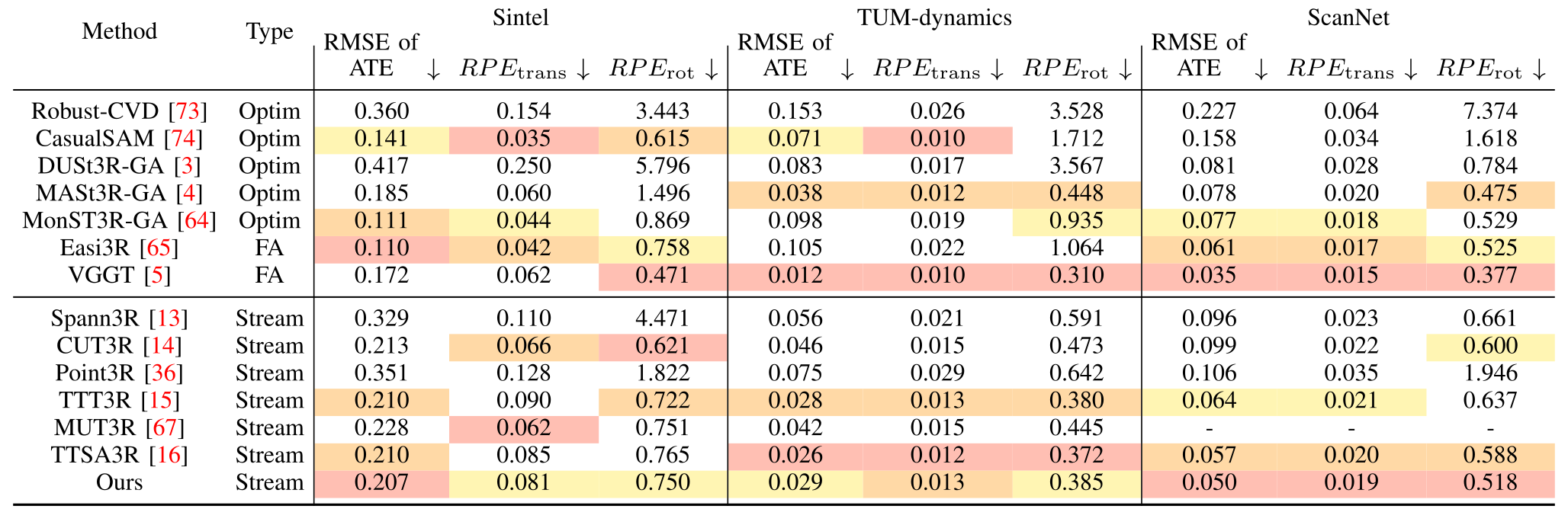
Accessible table and source citation links
| Method | Type | Sintel | TUM-dynamics | ScanNet | ||||||
|---|---|---|---|---|---|---|---|---|---|---|
| RMSE of ATE | RMSE of ATE | RMSE of ATE | ||||||||
| Robust-CVD [73] | Optim | 0.360 | 0.154 | 3.443 | 0.153 | 0.026 | 3.528 | 0.227 | 0.064 | 7.374 |
| CasualSAM [74] | Optim | 0.141 | 0.035 | 0.615 | 0.071 | 0.010 | 1.712 | 0.158 | 0.034 | 1.618 |
| DUSt3R-GA [3] | Optim | 0.417 | 0.250 | 5.796 | 0.083 | 0.017 | 3.567 | 0.081 | 0.028 | 0.784 |
| MASt3R-GA [4] | Optim | 0.185 | 0.060 | 1.496 | 0.038 | 0.012 | 0.448 | 0.078 | 0.020 | 0.475 |
| MonST3R-GA [64] | Optim | 0.111 | 0.044 | 0.869 | 0.098 | 0.019 | 0.935 | 0.077 | 0.018 | 0.529 |
| Easi3R [65] | FA | 0.110 | 0.042 | 0.758 | 0.105 | 0.022 | 1.064 | 0.061 | 0.017 | 0.525 |
| VGGT [5] | FA | 0.172 | 0.062 | 0.471 | 0.012 | 0.010 | 0.310 | 0.035 | 0.015 | 0.377 |
| Spann3R [13] | Stream | 0.329 | 0.110 | 4.471 | 0.056 | 0.021 | 0.591 | 0.096 | 0.023 | 0.661 |
| CUT3R [14] | Stream | 0.213 | 0.066 | 0.621 | 0.046 | 0.015 | 0.473 | 0.099 | 0.022 | 0.600 |
| Point3R [36] | Stream | 0.351 | 0.128 | 1.822 | 0.075 | 0.029 | 0.642 | 0.106 | 0.035 | 1.946 |
| TTT3R [15] | Stream | 0.210 | 0.090 | 0.722 | 0.028 | 0.013 | 0.380 | 0.064 | 0.021 | 0.637 |
| MUT3R [67] | Stream | 0.228 | 0.062 | 0.751 | 0.042 | 0.015 | 0.445 | - | - | - |
| TTSA3R [16] | Stream | 0.210 | 0.085 | 0.765 | 0.026 | 0.012 | 0.372 | 0.057 | 0.020 | 0.588 |
| Ours | Stream | 0.207 | 0.081 | 0.750 | 0.029 | 0.013 | 0.385 | 0.050 | 0.019 | 0.518 |
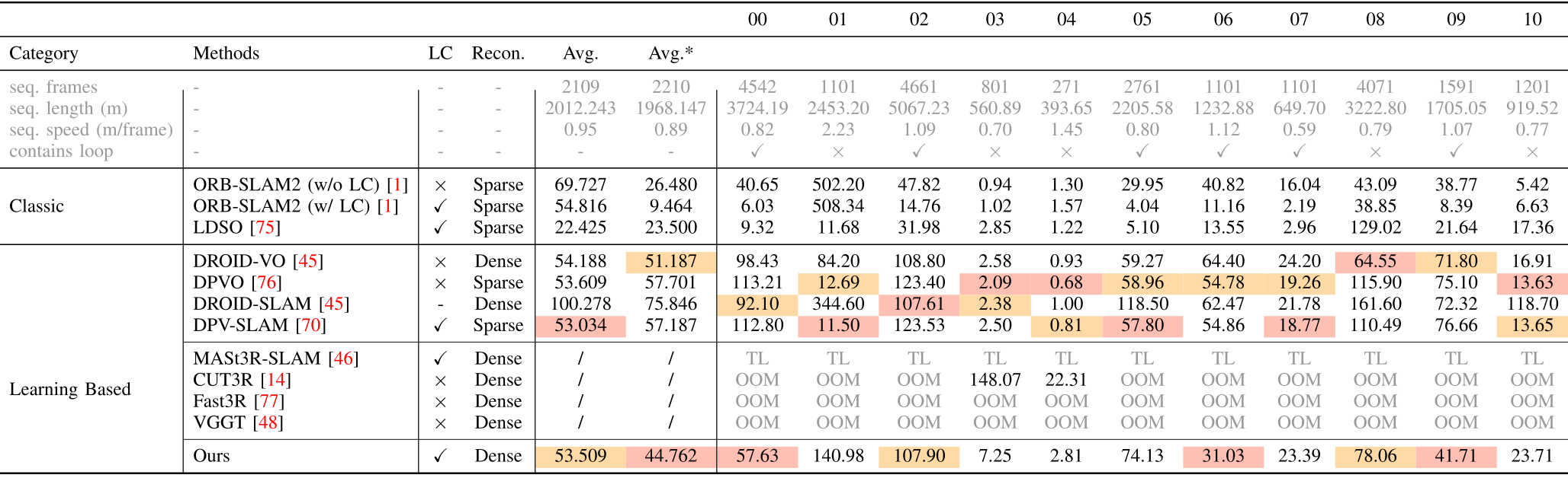
Accessible table and source citation links
00
01
02
03
04
05
06
07
08
09
10
Category
Methods
LC
Recon.
Avg.
Avg.*
seq. frames
-
-
-
2109
2210
4542
1101
4661
801
271
2761
1101
1101
4071
1591
1201
seq. length (m)
-
-
-
2012.243
1968.147
3724.19
2453.20
5067.23
560.89
393.65
2205.58
1232.88
649.70
3222.80
1705.05
919.52
seq. speed (m/frame)
-
-
-
0.95
0.89
0.82
2.23
1.09
0.70
1.45
0.80
1.12
0.59
0.79
1.07
0.77
contains loop
-
-
-
-
-
Classic
ORB-SLAM2 (w/o LC) [1]
Sparse
69.727
26.480
40.65
502.20
47.82
0.94
1.30
29.95
40.82
16.04
43.09
38.77
5.42
ORB-SLAM2 (w/ LC) [1]
Sparse
54.816
9.464
6.03
508.34
14.76
1.02
1.57
4.04
11.16
2.19
38.85
8.39
6.63
LDSO [75]
Sparse
22.425
23.500
9.32
11.68
31.98
2.85
1.22
5.10
13.55
2.96
129.02
21.64
17.36
Learning Based
DROID-VO [45]
Dense
54.188
51.187
98.43
84.20
108.80
2.58
0.93
59.27
64.40
24.20
64.55
71.80
16.91
DPVO [76]
Sparse
53.609
57.701
113.21
12.69
123.40
2.09
0.68
58.96
54.78
19.26
115.90
75.10
13.63
DROID-SLAM [45]
-
Dense
100.278
75.846
92.10
344.60
107.61
2.38
1.00
118.50
62.47
21.78
161.60
72.32
118.70
DPV-SLAM [70]
Sparse
53.034
57.187
112.80
11.50
123.53
2.50
0.81
57.80
54.86
18.77
110.49
76.66
13.65
MASt3R-SLAM [46]
Dense
/
/
TL
TL
TL
TL
TL
TL
TL
TL
TL
TL
TL
CUT3R [14]
Dense
/
/
OOM
OOM
OOM
148.07
22.31
OOM
OOM
OOM
OOM
OOM
OOM
Fast3R [77]
Dense
/
/
OOM
OOM
OOM
OOM
OOM
OOM
OOM
OOM
OOM
OOM
OOM
VGGT [48]
Dense
/
/
OOM
OOM
OOM
OOM
OOM
OOM
OOM
OOM
OOM
OOM
OOM
Ours
Dense
53.509
44.762
57.63
140.98
107.90
7.25
2.81
74.13
31.03
23.39
78.06
41.71
23.71
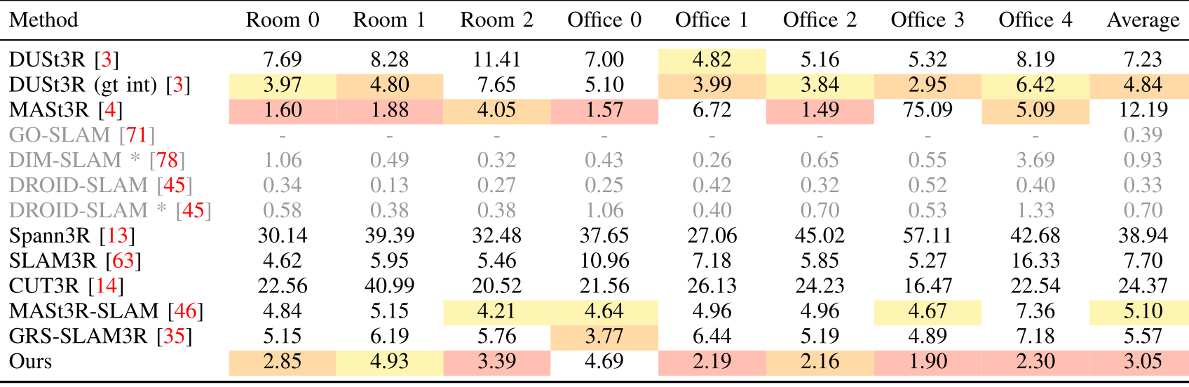
Accessible table and source citation links
| Method | Room 0 | Room 1 | Room 2 | Office 0 | Office 1 | Office 2 | Office 3 | Office 4 | Average |
|---|---|---|---|---|---|---|---|---|---|
| DUSt3R [3] | 7.69 | 8.28 | 11.41 | 7.00 | 4.82 | 5.16 | 5.32 | 8.19 | 7.23 |
| DUSt3R (gt int)[3] | 3.97 | 4.80 | 7.65 | 5.10 | 3.99 | 3.84 | 2.95 | 6.42 | 4.84 |
| MASt3R [4] | 1.60 | 1.88 | 4.05 | 1.57 | 6.72 | 1.49 | 75.09 | 5.09 | 12.19 |
| GO-SLAM [71] | - | - | - | - | - | - | - | - | 0.39 |
| DIM-SLAM *[78] | 1.06 | 0.49 | 0.32 | 0.43 | 0.26 | 0.65 | 0.55 | 3.69 | 0.93 |
| DROID-SLAM [45] | 0.34 | 0.13 | 0.27 | 0.25 | 0.42 | 0.32 | 0.52 | 0.40 | 0.33 |
| DROID-SLAM * [45] | 0.58 | 0.38 | 0.38 | 1.06 | 0.40 | 0.70 | 0.53 | 1.33 | 0.70 |
| Spann3R [13] | 30.14 | 39.39 | 32.48 | 37.65 | 27.06 | 45.02 | 57.11 | 42.68 | 38.94 |
| SLAM3R[63] | 4.62 | 5.95 | 5.46 | 10.96 | 7.18 | 5.85 | 5.27 | 16.33 | 7.70 |
| CUT3R [14] | 22.56 | 40.99 | 20.52 | 21.56 | 26.13 | 24.23 | 16.47 | 22.54 | 24.37 |
| MASt3R-SLAM [46] | 4.84 | 5.15 | 4.21 | 4.64 | 4.96 | 4.96 | 4.67 | 7.36 | 5.10 |
| GRS-SLAM3R [35] | 5.15 | 6.19 | 5.76 | 3.77 | 6.44 | 5.19 | 4.89 | 7.18 | 5.57 |
| Ours | 2.85 | 4.93 | 3.39 | 4.69 | 2.19 | 2.16 | 1.90 | 2.30 | 3.05 |
IV-D Dense Reconstruction Evaluation
On 7-Scenes, reported mean accuracy/completeness distances are 1.97/1.75 cm after alignment. NRGBD gives 0.055/0.063 in the table’s printed centimeter units; completeness ties MASt3R-GA, while the median errors are not best.
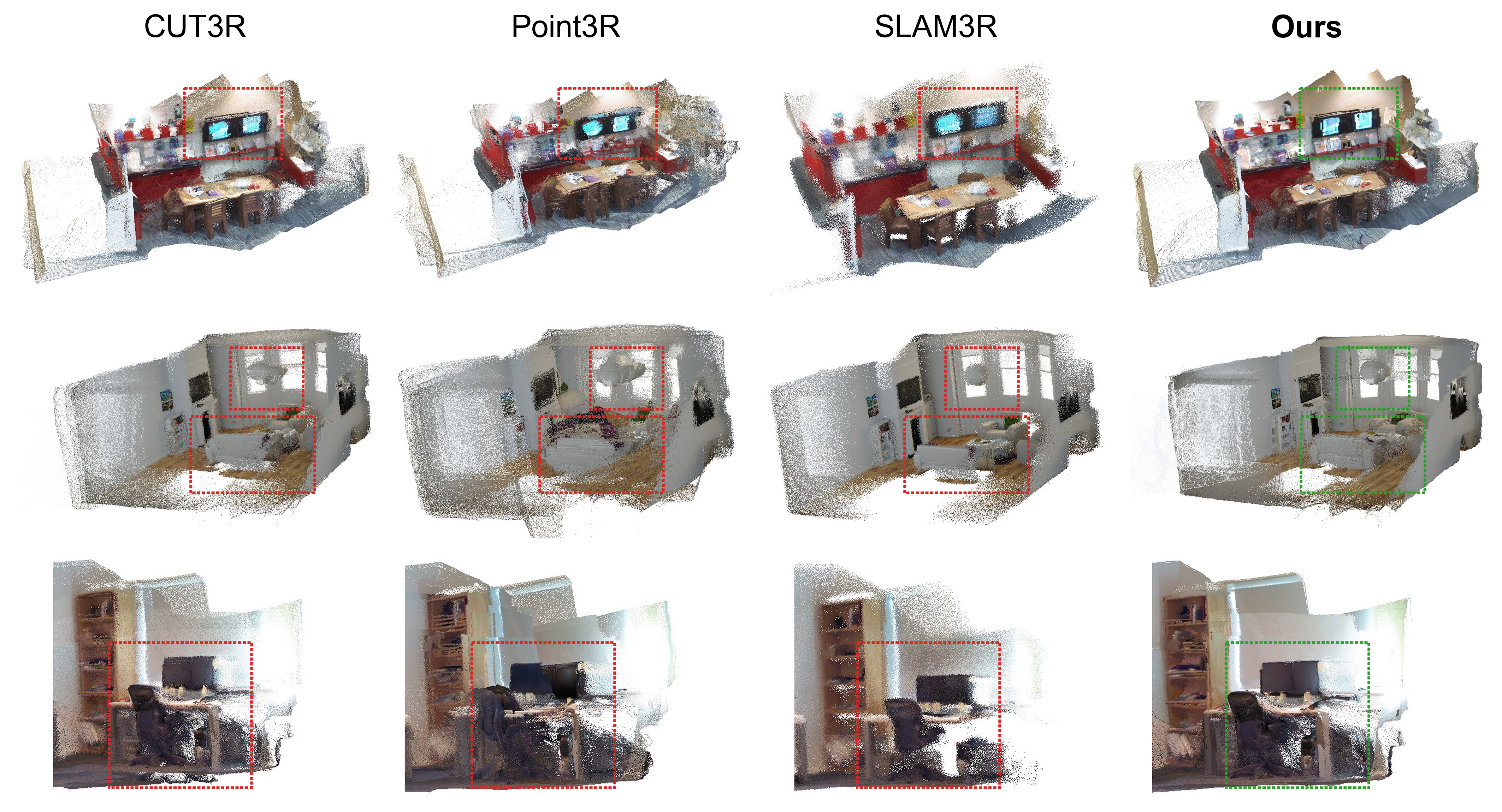
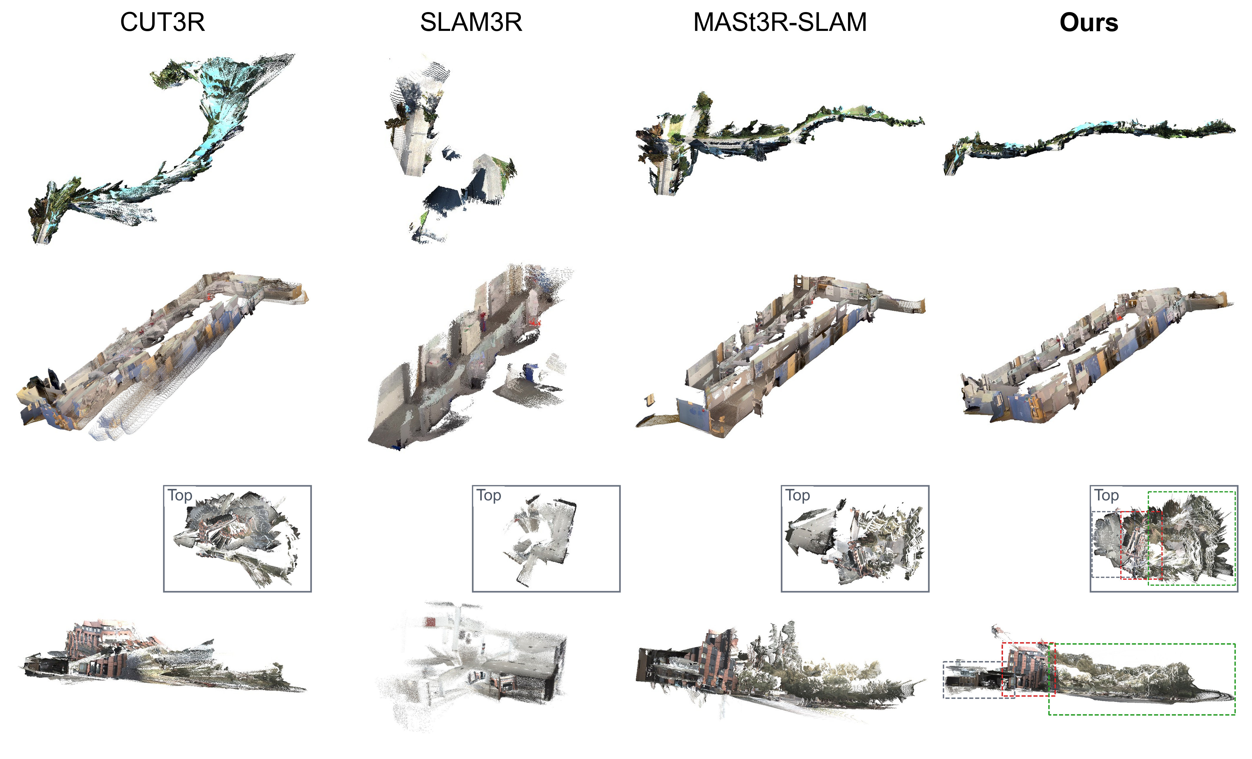
The NRGBD unit label is retained as printed rather than inferred from its unusually small magnitudes. Figures 3 and 4 show selected qualitative reconstructions, which do not measure failure rates or uncertainty across all scenes.

Accessible table and source citation links
Method
Chess
Fire
Heads
Office
Pumpkin
RedKitchen
Stairs
Average
Acc.
Comp.
Acc.
Comp.
Acc.
Comp.
Acc.
Comp.
Acc.
Comp.
Acc.
Comp.
Acc.
Comp.
Acc.
Comp.
DUSt3R[3]
2.26
2.13
1.04
1.50
1.66
0.98
4.62
4.74
1.73
2.43
1.95
2.36
3.37
10.75
2.19
3.24
MASt3R [4]
2.08
2.12
1.54
1.43
1.06
1.04
3.23
3.19
5.68
3.07
3.50
3.37
2.36
13.16
3.04
3.90
Spann3R [13]
2.23
1.68
0.88
0.92
2.67
0.98
5.86
3.54
2.25
1.85
2.68
1.80
5.65
5.15
3.42
2.41
CUT3R[14]
2.46
1.99
1.52
1.43
2.10
1.13
3.81
3.05
2.98
2.48
2.49
2.24
3.35
10.53
2.67
3.27
SLAM3R [63]
1.63
1.31
0.84
0.83
2.95
1.22
2.32
2.26
1.81
2.05
1.84
1.94
4.19
6.91
2.13
2.34
MASt3R-SLAM[46]
2.41
1.70
1.57
1.33
1.71
1.16
3.47
2.98
2.86
2.37
2.83
2.16
3.32
9.53
2.60
3.03
GRS-SLAM3R [35]
1.49
1.32
1.26
1.32
1.22
0.83
4.17
3.41
2.27
2.25
2.19
2.19
2.22
4.55
2.12
2.27
Ours
1.42
1.16
1.15
1.07
0.62
0.49
3.56
2.85
1.93
1.99
2.21
1.72
2.89
2.95
1.97
1.75
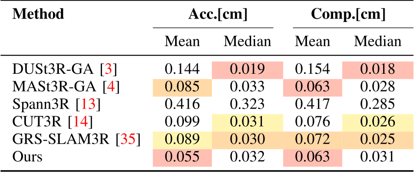
Accessible table and source citation links
| Method | Acc.[cm] | Comp.[cm] | ||
|---|---|---|---|---|
| Mean | Median | Mean | Median | |
| DUSt3R-GA [3] | 0.144 | 0.019 | 0.154 | 0.018 |
| MASt3R-GA [4] | 0.085 | 0.033 | 0.063 | 0.028 |
| Spann3R [13] | 0.416 | 0.323 | 0.417 | 0.285 |
| CUT3R [14] | 0.099 | 0.031 | 0.076 | 0.026 |
| GRS-SLAM3R [35] | 0.089 | 0.030 | 0.072 | 0.025 |
| Ours | 0.055 | 0.032 | 0.063 | 0.031 |
IV-E Gaussian Rendering Evaluation
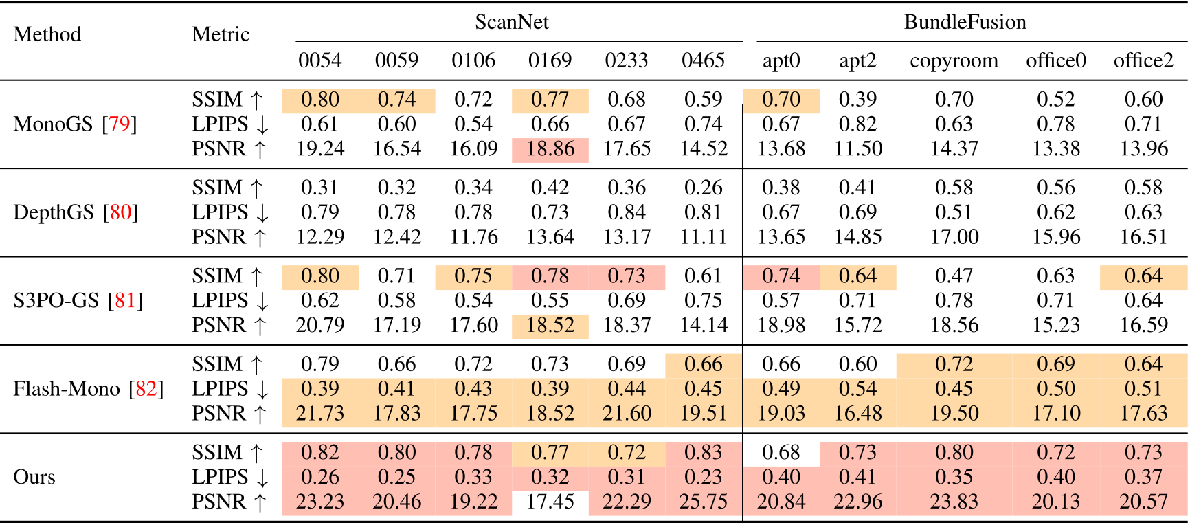
The method has the lowest listed LPIPS on all 11 rendering scenes and the highest PSNR on ten. ScanNet 0169 is an exception:17.45 dB is below several baselines. SSIM is also below alternatives on some scenes, including BundleFusion apt 0.
These comparisons support useful rendering quality alongside mapping. The paper does not fully specify held-out-view selection, repeat uncertainty or a matched-compute rendering comparison.
Accessible table and source citation links
| Method | Metric | ScanNet | BundleFusion | |||||||||
|---|---|---|---|---|---|---|---|---|---|---|---|---|
| 0054 | 0059 | 0106 | 0169 | 0233 | 0465 | apt0 | apt2 | copyroom | office0 | office2 | ||
| MonoGS[79] | SSIM | 0.80 | 0.74 | 0.72 | 0.77 | 0.68 | 0.59 | 0.70 | 0.39 | 0.70 | 0.52 | 0.60 |
| LPIPS | 0.61 | 0.60 | 0.54 | 0.66 | 0.67 | 0.74 | 0.67 | 0.82 | 0.63 | 0.78 | 0.71 | |
| PSNR | 19.24 | 16.54 | 16.09 | 18.86 | 17.65 | 14.52 | 13.68 | 11.50 | 14.37 | 13.38 | 13.96 | |
| DepthGS[80] | SSIM | 0.31 | 0.32 | 0.34 | 0.42 | 0.36 | 0.26 | 0.38 | 0.41 | 0.58 | 0.56 | 0.58 |
| LPIPS | 0.79 | 0.78 | 0.78 | 0.73 | 0.84 | 0.81 | 0.67 | 0.69 | 0.51 | 0.62 | 0.63 | |
| PSNR | 12.29 | 12.42 | 11.76 | 13.64 | 13.17 | 11.11 | 13.65 | 14.85 | 17.00 | 15.96 | 16.51 | |
| S3PO-GS[81] | SSIM | 0.80 | 0.71 | 0.75 | 0.78 | 0.73 | 0.61 | 0.74 | 0.64 | 0.47 | 0.63 | 0.64 |
| LPIPS | 0.62 | 0.58 | 0.54 | 0.55 | 0.69 | 0.75 | 0.57 | 0.71 | 0.78 | 0.71 | 0.64 | |
| PSNR | 20.79 | 17.19 | 17.60 | 18.52 | 18.37 | 14.14 | 18.98 | 15.72 | 18.56 | 15.23 | 16.59 | |
| Flash-Mono[82] | SSIM | 0.79 | 0.66 | 0.72 | 0.73 | 0.69 | 0.66 | 0.66 | 0.60 | 0.72 | 0.69 | 0.64 |
| LPIPS | 0.39 | 0.41 | 0.43 | 0.39 | 0.44 | 0.45 | 0.49 | 0.54 | 0.45 | 0.50 | 0.51 | |
| PSNR | 21.73 | 17.83 | 17.75 | 18.52 | 21.60 | 19.51 | 19.03 | 16.48 | 19.50 | 17.10 | 17.63 | |
| Ours | SSIM | 0.82 | 0.80 | 0.78 | 0.77 | 0.72 | 0.83 | 0.68 | 0.73 | 0.80 | 0.72 | 0.73 |
| LPIPS | 0.26 | 0.25 | 0.33 | 0.32 | 0.31 | 0.23 | 0.40 | 0.41 | 0.35 | 0.40 | 0.37 | |
| PSNR | 23.23 | 20.46 | 19.22 | 17.45 | 22.29 | 25.75 | 20.84 | 22.96 | 23.83 | 20.13 | 20.57 | |
IV-F Real-World Multi-Platform Evaluation
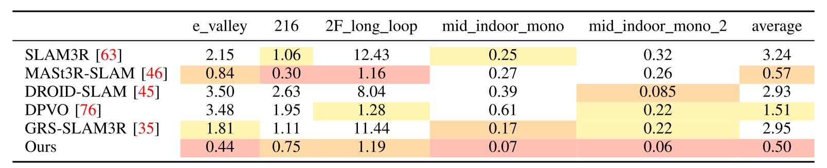
Five robot sequences give an average absolute trajectory error of 0.50 m, versus 0.57 m for MASt3R-SLAM. The method is best on three sequences and second on two. Selected visual comparisons extend to indoor–outdoor scenes.
This evaluates a subset of the 16 listed recordings. Difficult night sequences and every platform/scene combination do not each receive a numerical trajectory result, so robustness across the full collected set is not established by this table alone.
Accessible table and source citation links
| e_valley | 216 | 2F_long_loop | mid_indoor_mono | mid_indoor_mono_2 | average | |
|---|---|---|---|---|---|---|
| SLAM3R[63] | 2.15 | 1.06 | 12.43 | 0.25 | 0.32 | 3.24 |
| MASt3R-SLAM[46] | 0.84 | 0.30 | 1.16 | 0.27 | 0.26 | 0.57 |
| DROID-SLAM [45] | 3.50 | 2.63 | 8.04 | 0.39 | 0.085 | 2.93 |
| DPVO [76] | 3.48 | 1.95 | 1.28 | 0.61 | 0.22 | 1.51 |
| GRS-SLAM3R [35] | 1.81 | 1.11 | 11.44 | 0.17 | 0.22 | 2.95 |
| Ours | 0.44 | 0.75 | 1.19 | 0.07 | 0.06 | 0.50 |
IV-G Runtime and Memory Analysis
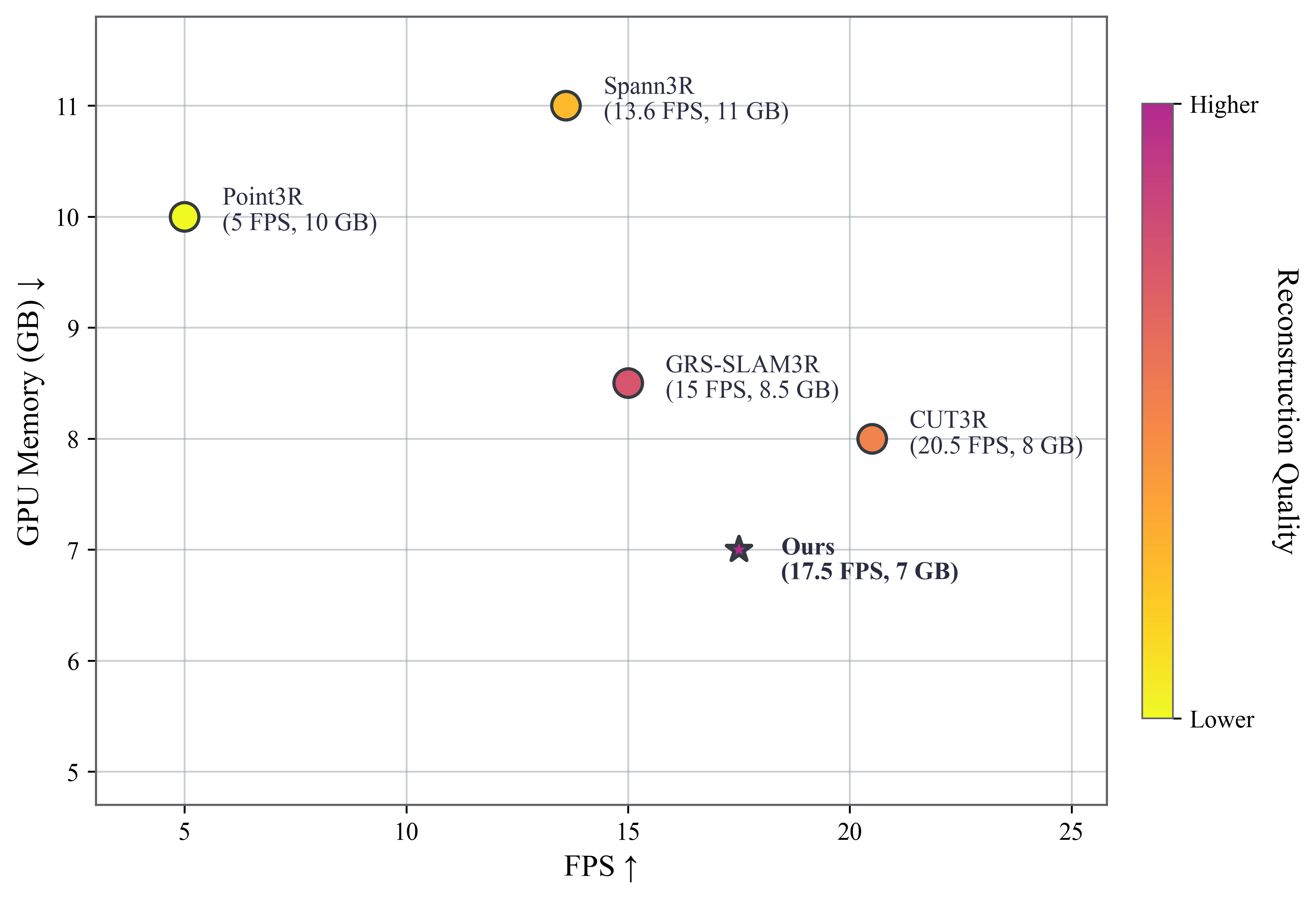
Figure 5 reports 17.5 frames per second and 7 GB GPU memory on an RTX 4090, with a qualitative reconstruction-quality color scale. This is a selected operating point, rather than a complete latency distribution or a sequence-length memory-growth curve.
The prose mentions component timing, but no numerical per-module timing table appears in this version. Persistent submaps and Gaussians still grow the stored map; fixed active memory does not prove bounded total storage over arbitrarily long operation.
IV-H Ablation Studies
On Apartment, temporal-only regulation gives 13.26/10.84 cm reconstruction errors and 0.49 m trajectory error; spatial-only gives 14.78/12.31 cm and 0.53 m. Combining both gives 9.14/7.30 cm and 0.38 m before loop closure.
With all components and submap size 16, results reach 5.88/4.52 cm and 0.12 m. Sizes 8 and 32 are slightly worse, supporting a moderate submap size for this dataset. Removing submaps causes the largest single-component degradation in the displayed comparison.
The table does not isolate every claimed component: there is no separate Gaussian-head ablation or rigid-versus-projective backend comparison. These results do not independently identify all sources of improvement.
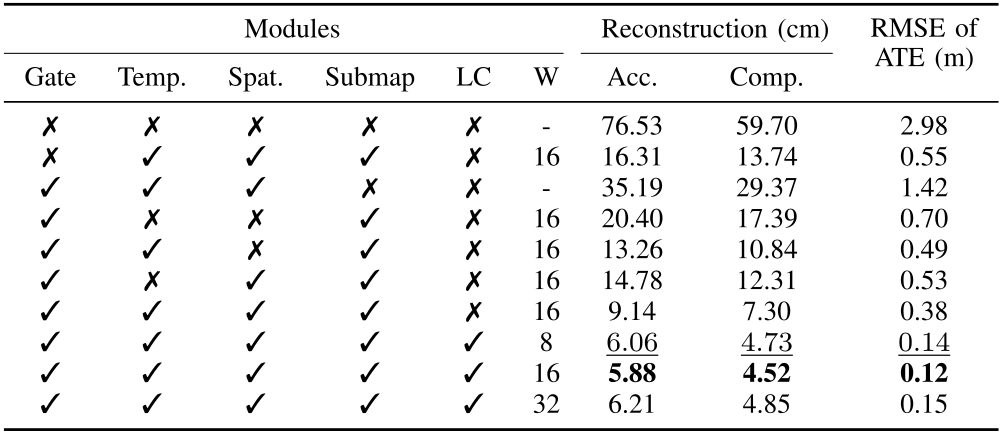
Accessible table and source citation links
| Modules | Reconstruction (cm) | RMSE of ATE (m) | ||||||
| Gate | Temp. | Spat. | Submap | LC | W | Acc. | Comp. | |
| ✗ | ✗ | ✗ | ✗ | ✗ | - | 76.53 | 59.70 | 2.98 |
| ✗ | ✓ | ✓ | ✓ | ✗ | 16 | 16.31 | 13.74 | 0.55 |
| ✓ | ✓ | ✓ | ✗ | ✗ | - | 35.19 | 29.37 | 1.42 |
| ✓ | ✗ | ✗ | ✓ | ✗ | 16 | 20.40 | 17.39 | 0.70 |
| ✓ | ✓ | ✗ | ✓ | ✗ | 16 | 13.26 | 10.84 | 0.49 |
| ✓ | ✗ | ✓ | ✓ | ✗ | 16 | 14.78 | 12.31 | 0.53 |
| ✓ | ✓ | ✓ | ✓ | ✗ | 16 | 9.14 | 7.30 | 0.38 |
| ✓ | ✓ | ✓ | ✓ | ✓ | 8 | |||
| ✓ | ✓ | ✓ | ✓ | ✓ | 16 | 5.88 | 4.52 | 0.12 |
| ✓ | ✓ | ✓ | ✓ | ✓ | 32 | 6.21 | 4.85 | 0.15 |
V Conclusion
The paper connects adaptive recurrent state, submap-level correction and feed-forward Gaussian prediction in one streaming mapping system. Its strongest evidence is the collection of within-protocol benchmark comparisons and Apartment ablations.
Several numerical and reporting limitations constrain broader claims. Semantic/dynamic reasoning and downstream robot tasks remain future work; long-term reliability, total storage scaling and exact reproduction need further evidence.