Overview
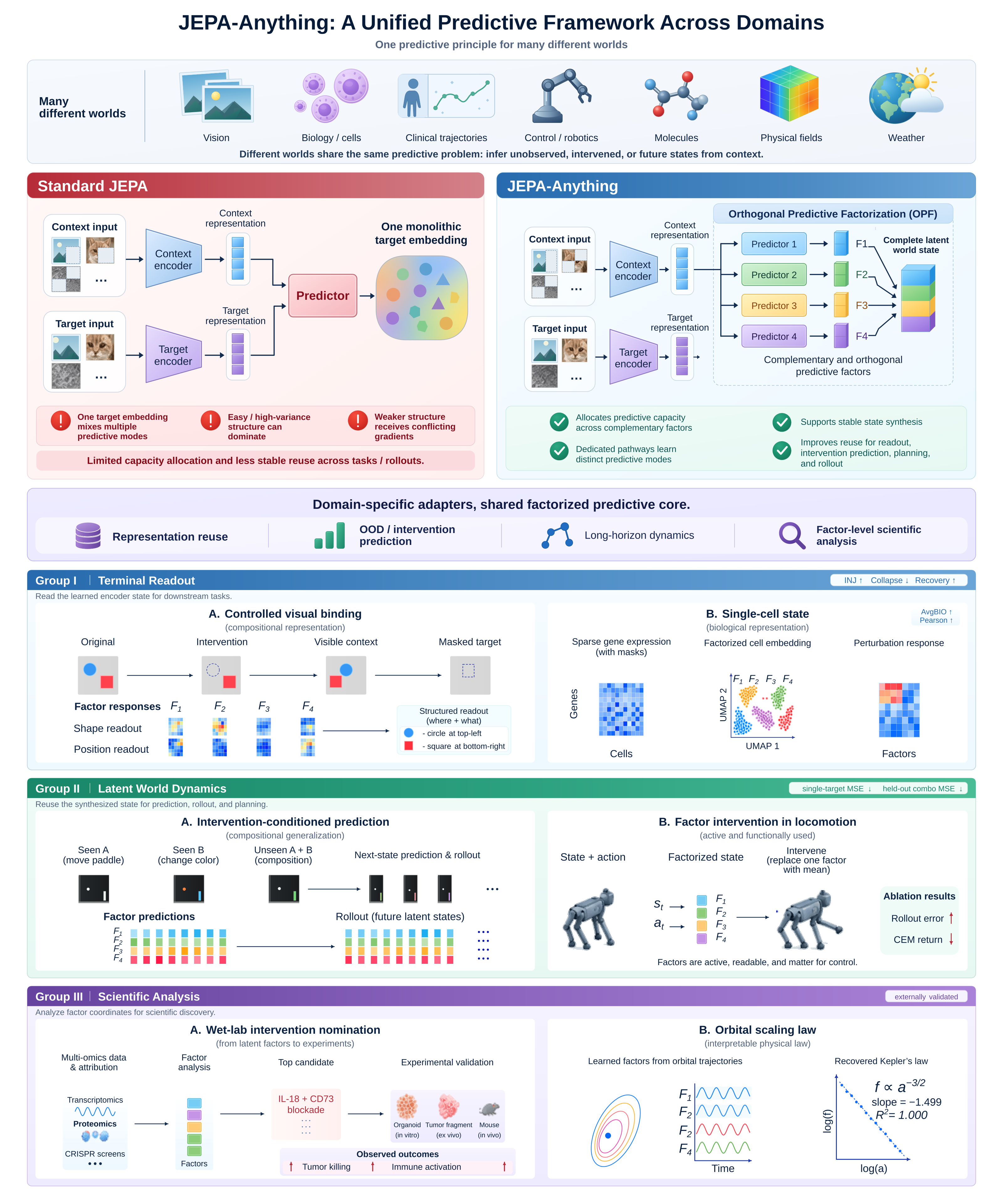
The figure summarizes the shared predictive interface and its evaluation modes.
At a glance
JEPA-Anything is a common learning framework instantiated separately across seven domains, not one jointly trained universal model. It splits latent prediction into orthogonal factors and recombines them into a complete state. Matched experiments report improved prediction across ten dynamics tasks and four molecular systems. Planning improves in two of three locomotion environments. Scientific demonstrations examine preclinical biological interventions and orbital scaling.
1 Introduction
A single latent target can let easy or high-variance features dominate learning. OPF allocates prediction capacity to complementary subspaces while domain-specific adapters determine observations and context–target relationships. The learned state can support a terminal readout, repeated transitions, or factor-level analysis. Shared architecture does not imply shared cross-domain coordinates or causal meaning.
Related references: [12], [14], [3], [6], [5], [20], [8], [13].
2 JEPA-Anything
2.1 One Interface, One Predictive Core
Adapters turn each domain’s data into tokens and structural descriptors, then select a predictive context and target. An online encoder represents context; an EMA encoder supplies stopped-gradient targets. A valid task requires a meaningful statistical relationship between states of the same system.
Equations 1–2
| (1) |
| (2) |
| Component | Domain-specific boundary | Shared JEPA-Anything core |
| Raw representation | Image, sequence, graph, set, record | — |
| Tokenization and descriptors | Common token interface | |
| Context–target semantics | Context predicts targets | |
| Encoder architecture | ViT, Transformer, GNN, MLP, | Online/EMA-target scheme |
| Predictive learning | — | Factorized predictors and state synthesis |
| Regularization | — | Orthogonality, factor activity, encoder variance |
| Training objective | Original loss | Additive OPF loss in Equation (10) |
| Downstream use | Pooling, readout, probe, decoder, planner | Online-encoder features or synthesized predicted states |
2.2 Orthogonal Predictive Factorization
Learned projectors partition the target into K factors, each predicted by a dedicated branch. A pseudoinverse reconstructs the complete latent state for decoding or rollout. Within-factor and cross-factor orthogonality penalties discourage degenerate or redundant bases. Exact orthogonality preserves information and avoids amplification of coordinate error; arbitrary multi-head predictors lack that guarantee.
Related references: [36], [7].
Equations 3–8
| (3) |
| (4) |
| (5) |
| (6) |
| (7) |
| (8) |
2.3 Maintaining Factor and Encoder Activity
A factor-variance floor keeps projected coordinates active, while a separate variance term directly prevents the online encoder from collapsing. Factor prediction and regularization are added to each domain implementation’s original objective.
Equations 9–10
| (9) | ||||
| (10) | ||||
2.4 Shared Predictive Pretraining and Task-Specific Readout
All domains follow the same sequence: adapt observations, sample views, encode context and targets, predict factors, update online parameters, and update the target encoder by EMA.
Representation mode.
For ordinary representation tasks, retain the online encoder and attach a task-specific readout. Target encoders and factor predictors are no longer needed at inference.
Equation 11
| (11) |
Operational world-model mode.
For forecasting and planning, retain the factor predictors and synthesis map so predicted states can be reused recursively. The projectors also expose coordinates for intervention and spectral analyses.
Equation
3 Experiments
Evaluation distinguishes terminal representations, recursive dynamics and planning, and scientific analysis of learned factors.
3.1 Common Evaluation Logic
Direct JEPA comparisons hold adapters, encoders, data splits, optimization budgets, and readouts fixed. Domain-specific metrics are reported separately rather than averaged across incompatible units. Control uses five training seeds and matched resets.
| Group/domain and data | Context target or analysis | Backbone or interface | OPF setup / interface | Seeds / splits / metrics |
| I / vision; controlled MuJoCo scenes | Visible patches masked patch states | DINOv3 ViT-S SigLIP2 Base | 10 seeds; image-disjoint and leave-one-cell-out; INJ, Coll., Rec. | |
| I / single cell; kidney, PBMC-10K, Adamson, Norman | Representation: masked expression complete cell state; Norman: target | scGPT | Norman: | 5 seeds; kidney pretraining; PBMC fine-tuned/zero-shot and cross-dataset perturbation transfer; AvgBIO, Pearson |
| I / clinical; longitudinal multimodal cohort | Patient history future patient state | GPT-2 small; risk decoder | 5 seeds; fixed patient-level cohort split; more than 1,000 event risks; PRAUC | |
| II / intervention; CITRIS Interventional Pong | Observation + intervention next state | Matched encoder and predictor | 5 paired seeds; single- and combined-intervention one-step prediction; six-step free rollout; four-channel MSE | |
| II / dynamics; CausalWorld, DMC, PDEBench, WeatherBench2 | State, frames, action, or forcing next state or field | Matched task-specific encoder and transition | 5 seeds; held-out/OOD and 6-step rollout; MSE and return | |
| II / PDE audit; APEBench Burgers and KS | Current field next field | MLP; first-layer weight | 5 paired seeds; held-out late-state prediction; Burgers 6-step rollout; MSE | |
| II / long rollout; 1-D viscous Burgers, 64 points | Current field autoregressive future field | MLP; input ; hidden width 256 | 3 seeds; 2,000 training steps; ID/high-frequency OOD at H20/H50; MSE | |
| II / locomotion; Hopper, Walker2d, HalfCheetah | State + action future control state | Latent dynamics; CEM planner | 5 seeds; matched resets and 20-step factor interventions; return, , MSE | |
| II / molecules; water, quartz, paracetamol, benzene | Atomic state future molecular state | TrajCast-style equivariant; sector | (channels) | 5 seeds; 100-step free rollout; MAE, RMSD |
| III / biology; Huh7–PBMC, organoids, tumor fragments, mice | Factor coordinates candidate intervention nomination | OPF factor-analysis interface | Retained | 3 organoids and 3 fragments plus external mouse validation; killing and activation |
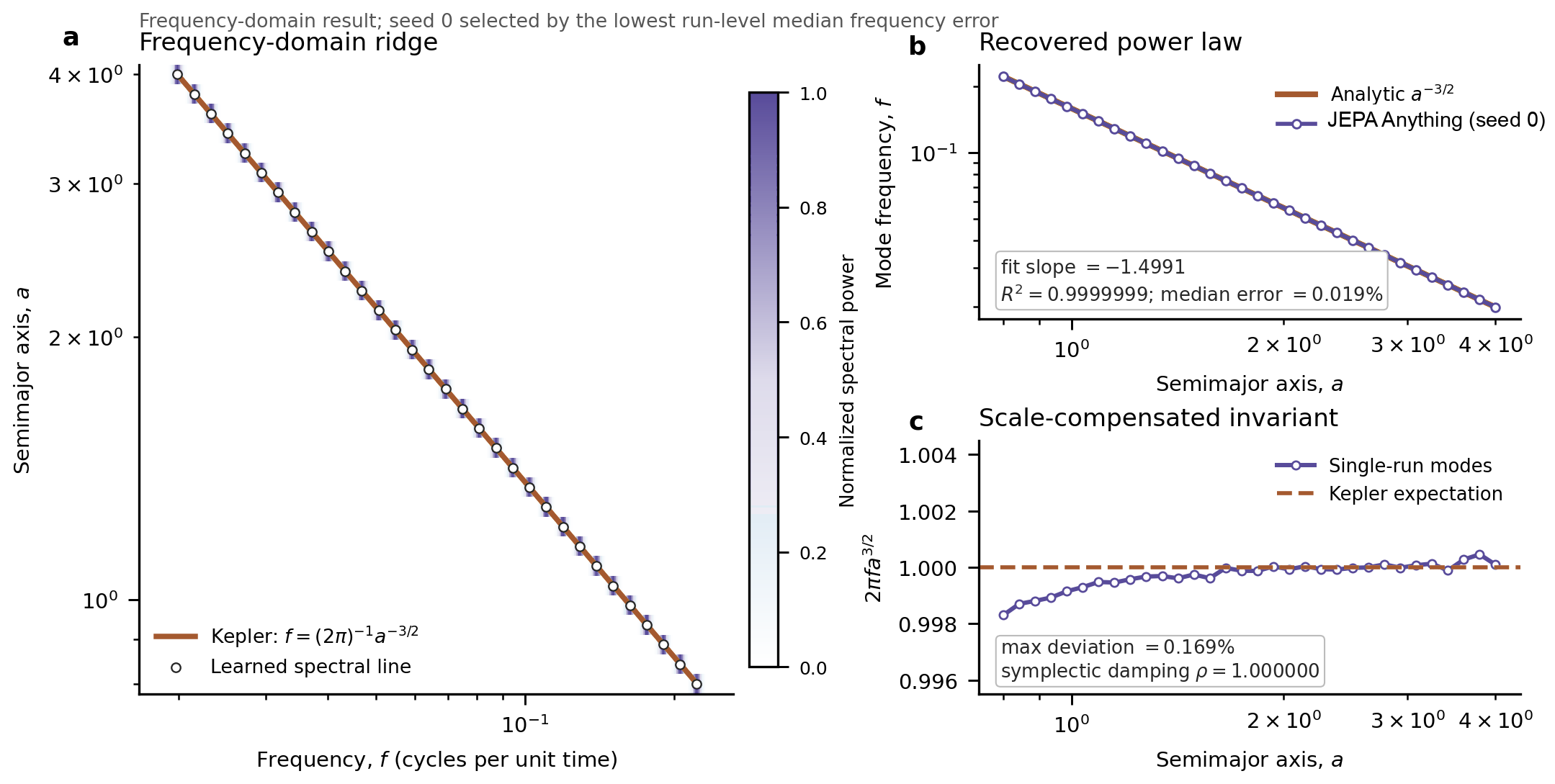
| III / orbital; simulated position–velocity trajectories | Factor coordinates latent spectral modes | Trajectory encoding; spectral analysis | Retained | One analyzed run with analytic-law validation; slope and |
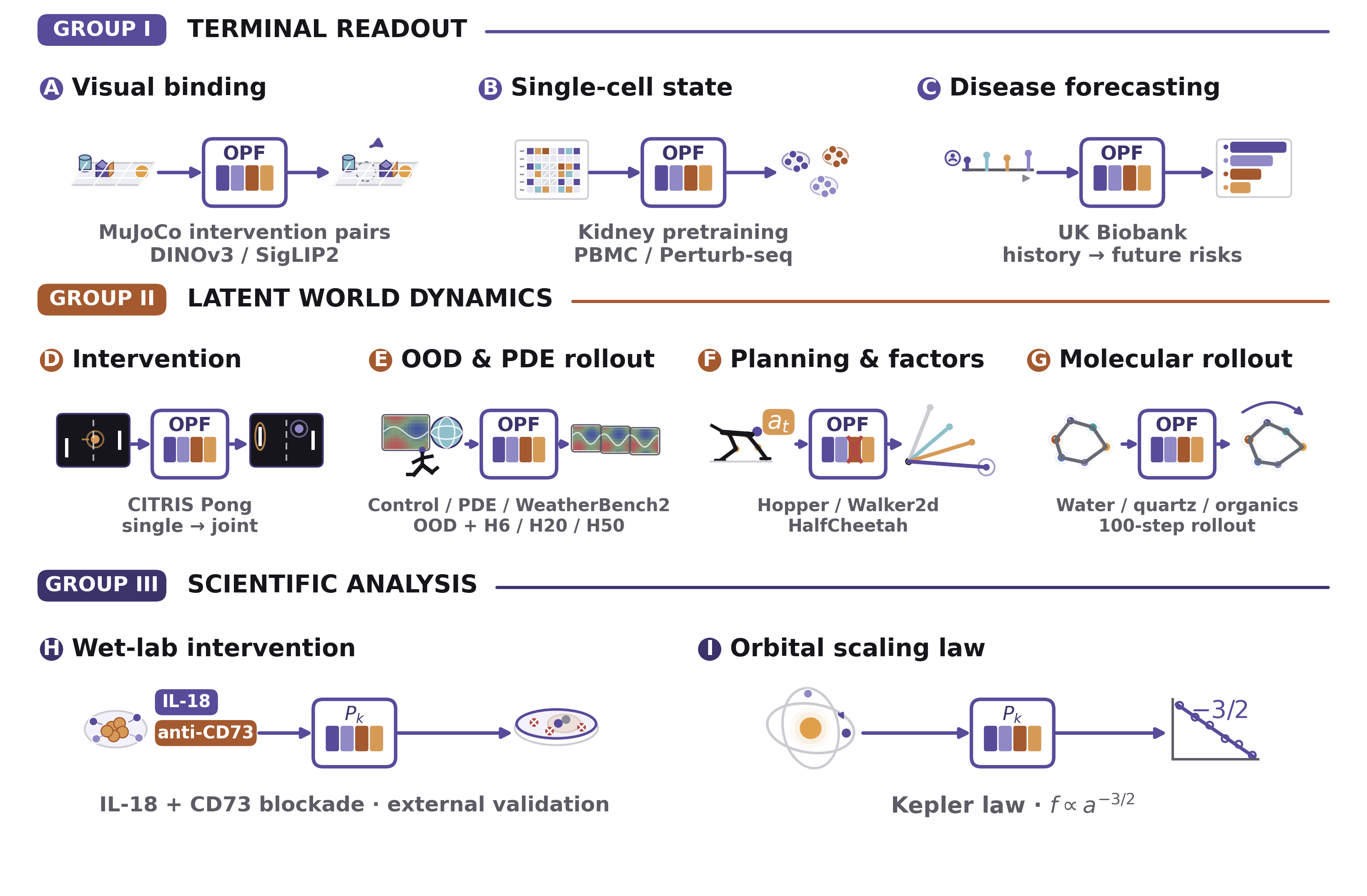
3.2 Group I: Terminal Readout of Predictive World States
Vision and cell tasks read the trained encoder; disease forecasting reads a synthesized future state. These tests terminate at a readout rather than repeatedly feeding predictions back.
3.2.1 Controlled Visual Binding
Question.
The visual task asks whether frozen features retain both the location and type of an image change, including combinations excluded from readout training.
Predictive pretraining.
DINOv3 and SigLIP2 checkpoints are pretrained with matched masked-patch tasks. Four-factor OPF replaces the monolithic JEPA target; the resulting encoders are then frozen.
Readout and evaluation.
Image-disjoint, held-out-cell evaluation measures binding accuracy, collapse, and recovered grid structure over ten seeds. OPF improves both backbones under the same learned-grid readout.
Related references: [32], [19].
| Backbone | Encoder pretraining | Grid supervision | INJ | Coll. | Rec. |
|---|---|---|---|---|---|
| DINOv3 | Frozen checkpoint | Known grid | .452 | .667 | — |
| DINOv3 | Frozen checkpoint | Learned grid | .569 | .433 | .643 |
| DINOv3 | Standard JEPA | Learned grid | .572 | .426 | .645 |
| DINOv3 | JEPA-Anything | Learned grid | .581 | .417 | .659 |
| SigLIP2 | Frozen checkpoint | Known grid | .476 | .656 | — |
| SigLIP2 | Frozen checkpoint | Learned grid | .484 | .511 | .676 |
| SigLIP2 | Standard JEPA | Learned grid | .483 | .514 | .679 |
| SigLIP2 | JEPA-Anything | Learned grid | .490 | .503 | .688 |
3.2.2 Single-Cell State Representation and Perturbation Prediction
Question.
Latent prediction aims to retain cellular state while reducing sensitivity to sparse expression counts and technical dropout.
Protocol.
The cell experiments use a Cell-JEPA-style masked scGPT encoder. Perturbation prediction factorizes the response relative to a control cell into four 128-dimensional factors before decoding expression changes.
Evaluation.
Pretraining uses about 800,000 kidney cells. Evaluation covers PBMC clustering and Adamson/Norman perturbation prediction over five seeds; the factorized model leads the compared metrics in the reported table.
Related references: [1], [24].
| Model | JEPA | Orthogonal factors | PBMC finetuned AvgBIO | PBMC zero-shot AvgBIO | Norman Pearson | Adamson Pearson |
|---|---|---|---|---|---|---|
| scGPT | No | No | 0.7531 | 0.5288 | 0.631 | 0.905 |
| Cell-JEPA | Yes | No | 0.7830 | 0.7194 | 0.787 | 0.937 |
| JEPA-Anything | Yes | Yes | 0.8301 | 0.7752 | 0.814 | 0.942 |
3.2.3 Longitudinal Disease-State Forecasting
Question.
Clinical forecasting tests whether a latent future state predicts events from sparse, irregular patient histories.
Protocol.
A GPT-2-small encoder represents past history and an EMA encoder represents future states. Four factors reconstruct a future representation used by a shared decoder for more than 1,000 event risks.
Related references: [25].
Evaluation.
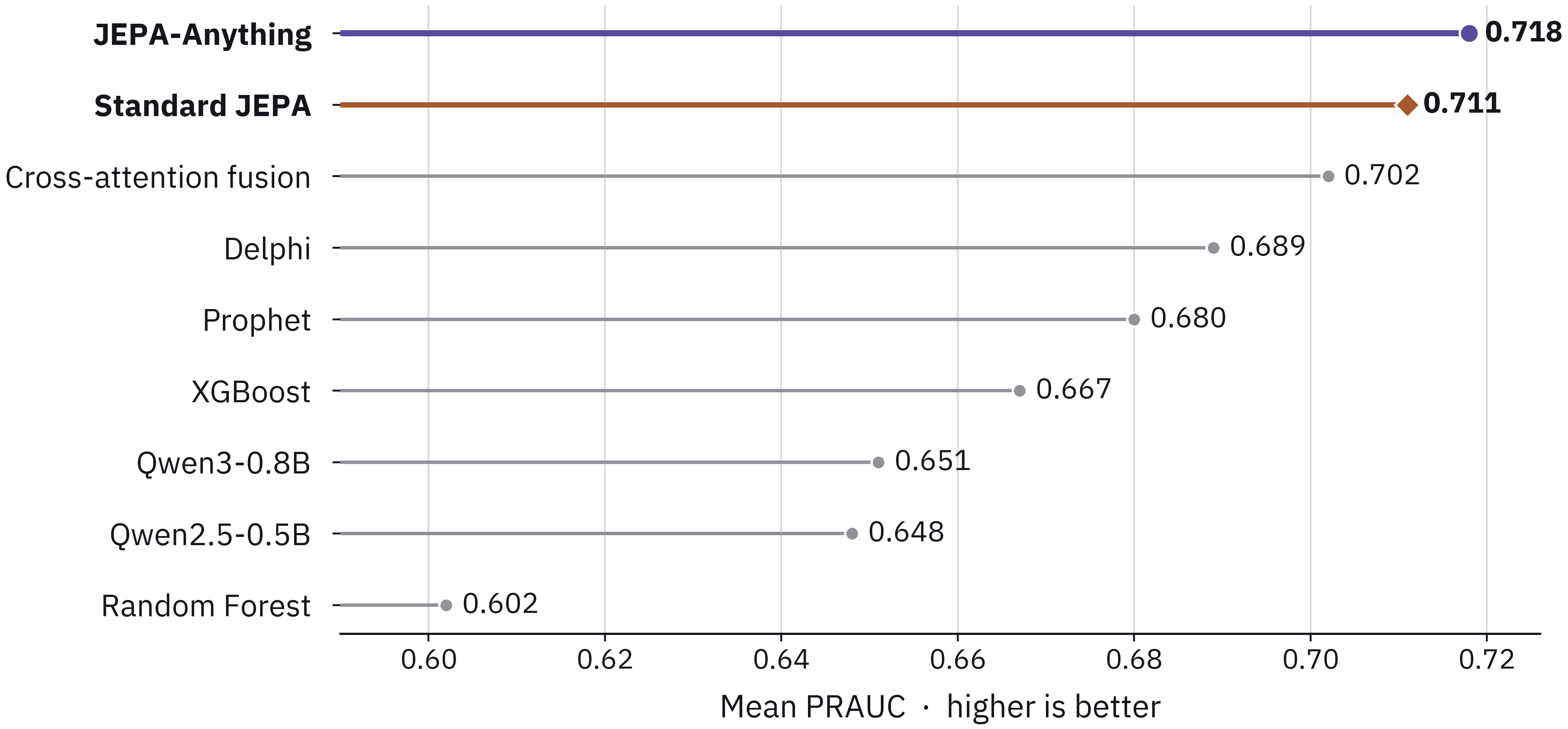
Mean PRAUC across the event vocabulary improves over a matched monolithic JEPA on a fixed patient-level split and five training seeds. This is retrospective predictive evaluation.
3.3 Group II: Latent World Dynamics and Rollout Stability
Recursive prediction tests whether errors remain controlled when synthesized latent states drive later forecasts or planning decisions.
3.3.1 Intervention-Conditioned Compositional Prediction
Question.
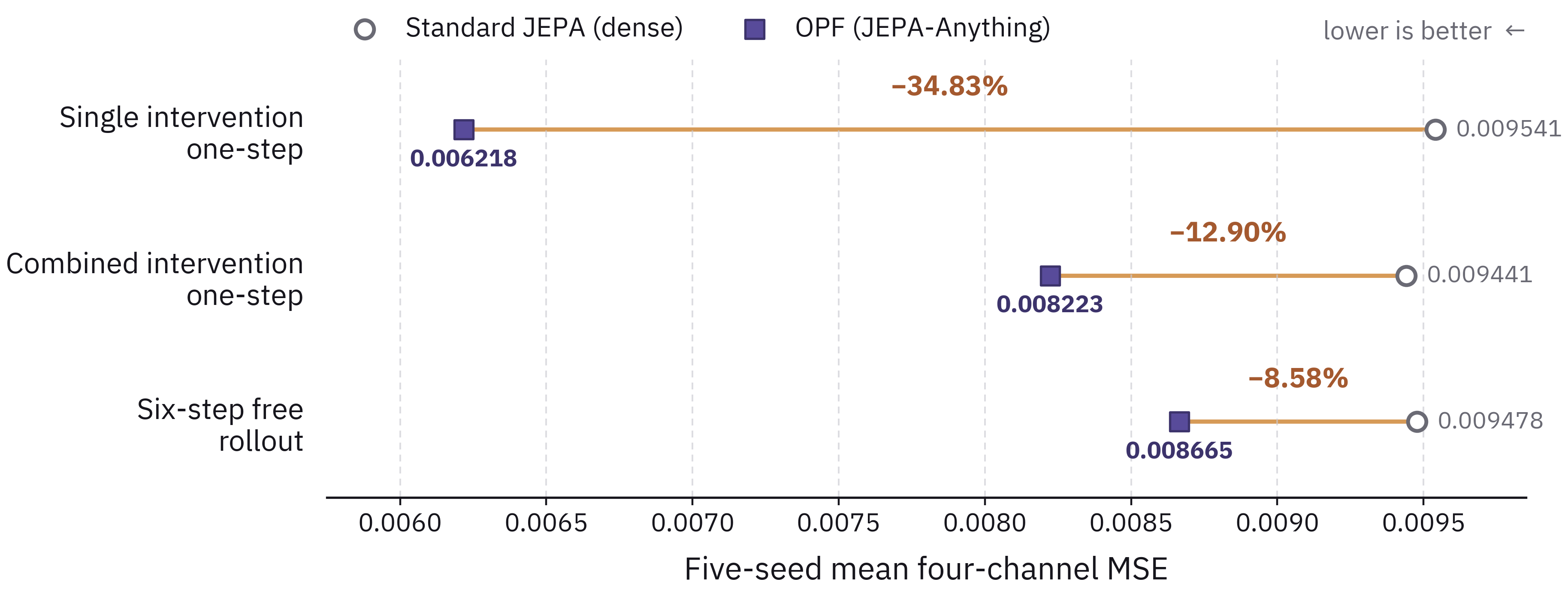
Interventional Pong supplies a pre-intervention state and labels of the changed factors. Evaluation covers seen single interventions, unseen combinations, and six-step free rollout.
Related references: [21].
Protocol and evaluation.
Against the matched dense JEPA, mean MSE falls from 0.009541 to 0.006218 for single interventions, 0.009441 to 0.008223 for unseen combinations, and 0.009478 to 0.008665 for six-step rollout: reductions of 34.83%, 12.90%, and 8.58%.
Orthogonality mechanism audit.
A capacity-matched multi-head audit measures subspace overlap, singular values, conditioning, synthesis error, and factor activity. Its exact-coordinate reconstruction test isolates geometry from prediction error; it is distinct from the forecasting benchmark.
| Metric | Unconstrained multi-head | Orthogonal factorization |
|---|---|---|
| Cross-factor subspace overlap | ||
| Minimum singular value | ||
| Condition number | ||
| Transpose synthesis NMSE (exact factors) |
3.3.2 Out-of-Distribution and Long-Horizon Dynamics
Question.
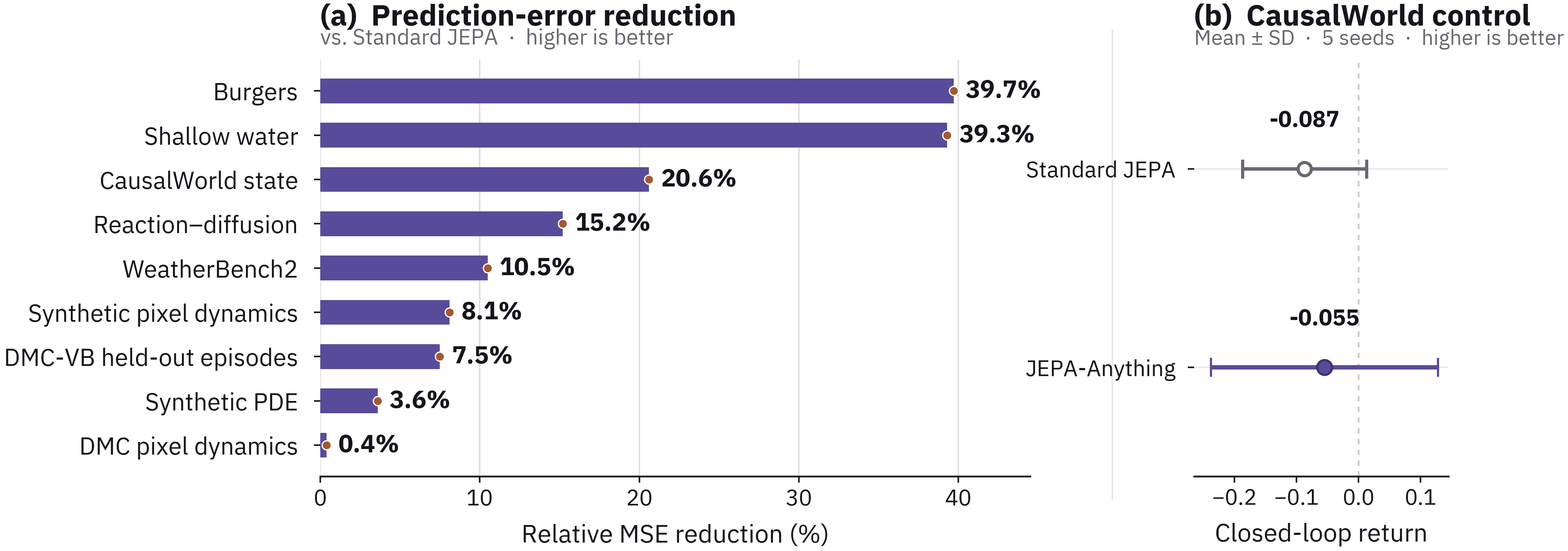
The ten-task dynamics suite tests unseen initial states, episodes, or periods and then six-step recursive prediction across visual, control, physical-field, and weather systems.
Protocol.
Both variants share data, backbones, budgets, splits, and five seeds within each task. Rollouts use the true action or target sequence. Weather normalization uses training-period statistics only.
Rollout and factor diagnostics.
The original table reports first- and sixth-step errors for representative systems, exposing error accumulation.
| Standard JEPA | JEPA-Anything | |||
|---|---|---|---|---|
| Task | Step 1 | Step 6 | Step 1 | Step 6 |
| CausalWorld state prediction | 0.01306 | 0.01307 | 0.01037 | 0.01079 |
| DMC pixel dynamics | 0.008539 | 0.008594 | 0.008498 | 0.008526 |
| PDEBench Burgers | 0.001830 | 0.006369 | 0.001101 | 0.004014 |
| PDEBench shallow water | 0.007090 | 0.010510 | 0.003999 | 0.006522 |
Additional APEBench evaluation.
Under the separate APEBench protocol, Burgers errors decrease about 49.5% on held-out late states and 44.7% over six steps; KS late-state error decreases about 13.2%. Improvements occur in every tested seed.
Related references: [18].
Capacity-matched Burgers long-rollout evaluation.
A capacity-matched Burgers experiment extends evaluation to 50 steps and high-frequency OOD trajectories. Gains persist but narrow with horizon. Routing diagnostics across nine tasks show about 3.782 effective factors out of four.
3.3.3 Continuous-Control Planning
Question.
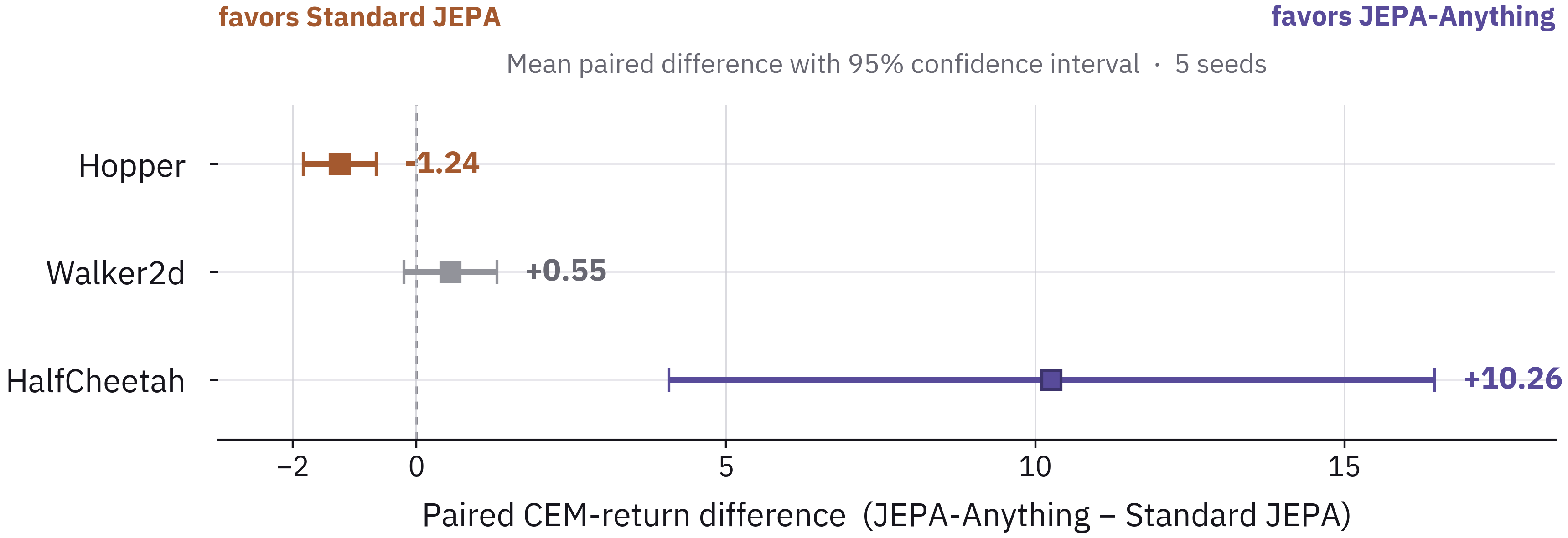
A CEM planner scores candidate action sequences through the learned model, then executes the first action of the best sequence. Real-environment return measures whether improved predictions lead to better decisions.
Protocol.
Matched Hopper, Walker2d, and HalfCheetah experiments use five training seeds and matched environment resets and planner randomness. OPF improves mean return on Walker2d and HalfCheetah, while standard JEPA performs better on Hopper. Benefits are environment-dependent.
Related references: [32].
3.3.4 Factor Activity and Functional Interventions in Locomotion
Question and protocol.
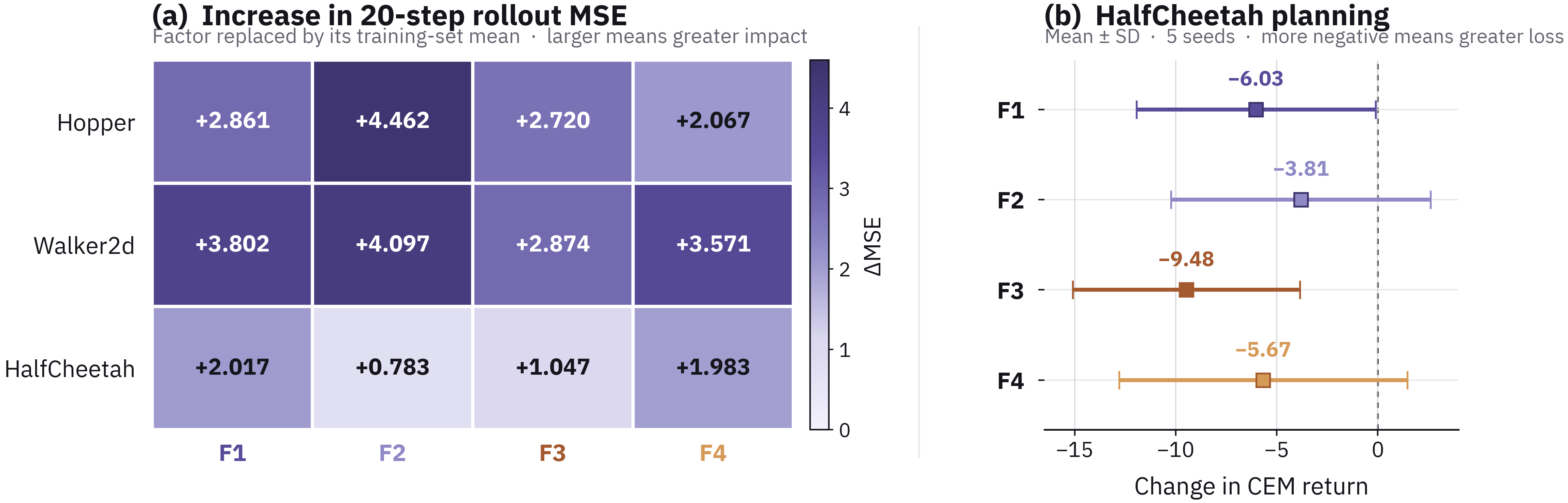
Factor probes, activity measurements, and interventions test whether each of four eight-dimensional state subspaces carries useful locomotion information.
Descriptive readout.
Individual factors show different linear-readout preferences for body height and joint angles. These are learned statistical preferences rather than fixed semantic labels.
Activity and intervention.
All factors remain active. Replacing any one by its training-set mean increases 20-step rollout error in all three environments; planning return also often declines. This supports functional use of each factor without establishing causal disentanglement.
3.3.5 Force-Free Molecular Forecasting
Question.
Force-free molecular forecasts recursively predict positions and velocities, making long-horizon error an essential complement to one-step accuracy.
Protocol.
Matched equivariant models are evaluated on water, quartz, paracetamol, and benzene. Factorization acts on feature multiplicity channels identically across vector components, preserving rotational equivariance.
Related references: [31].
Evaluation.
Across five seeds, JEPA-Anything has the lowest one-step displacement MAE and median final-position RMSD after 100 steps among the compared methods in all four systems.
| System | Metric | Scratch | TrajCast-JEPA | JEPA-Anything |
|---|---|---|---|---|
| Water | MAE | 0.00387 | 0.00452 | 0.00376 |
| Water | RMSD | 3.331 | 2.536 | 2.459 |
| Quartz | MAE | 0.01080 | 0.01043 | 0.01011 |
| Quartz | RMSD | 2.089 | 1.912 | 1.877 |
| Paracetamol | MAE | 0.00901 | 0.00777 | 0.00705 |
| Paracetamol | RMSD | 3.155 | 1.868 | 1.776 |
| Benzene | MAE | |||
| Benzene | RMSD | 0.0958 | 0.0701 | 0.0645 |
3.4 Group III: Scientific Analysis of Learned World States
The scientific demonstrations connect learned factor coordinates to biological experiments and a known physical scaling law.
3.4.1 Wet-Lab Evaluation of a Factor-Nominated Intervention
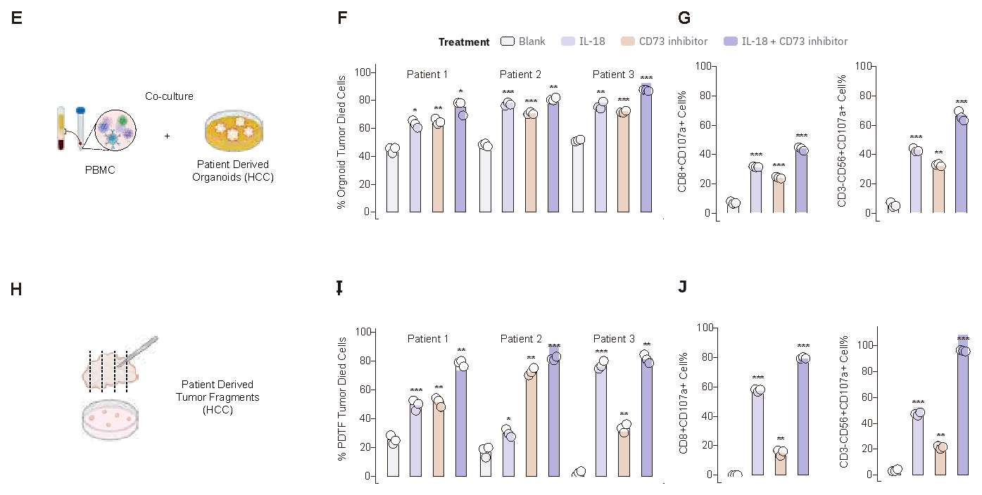
Factor analysis nominated IL-18 with NT5E/CD73 blockade. The authors report enhanced antitumor activity in co-cultures, patient-derived organoids and tumor fragments, and mice. These are preclinical findings, not evidence of clinical efficacy.
3.4.2 Orbital Scaling as a Physical-Law Diagnostic
Spectral analysis of simulated orbital trajectories recovers the frequency–semimajor-axis exponent at −1.4991, close to the Keplerian value −1.5. This tests whether latent modes retain a known physical regularity.
4 Related Work
Latent world models and planning.
Earlier latent world models primarily develop representations and transitions for visual prediction or control; this work applies a common factorized objective across broader domains.
Joint-embedding predictive learning.
Joint-embedding methods predict representations rather than raw observations. Their learned invariances still depend on the selected context–target relation.
Structured and factorized representations.
Object slots and causal factors require appropriate structure or supervision. OPF does not assume its predictive subspaces correspond to independent semantic causes.
Redundancy reduction and collapse prevention.
The method extends redundancy reduction with constraints on target-subspace bases, explicit activity terms, and a synthesis map for complete latent states.
5 Summary
A shared factorized objective supports several domain-specific prediction pipelines. Results favor it across many forecasting tasks, with mixed planning outcomes and separate biological and physical demonstrations.
6 Future Work
Future scientific-agent applications require calibrated uncertainty, reliable experiment selection, and revision under new evidence. Orthogonality alone establishes neither causality nor aligned representations across domains.
Appendix A Approximate Pseudoinverse-Synthesis Stability
When the learned basis is approximately orthogonal, its singular values bound the amplification of factor-prediction error. Pseudoinverse synthesis exactly reconstructs exact coordinates when the basis is invertible; the displayed proof states the assumptions.
Equations 12–13
| (12) |
| (13) |
Appendix B Supplementary Reproducibility Information
B.1 Implementation Details
The physical-field models use four factors in a 128-dimensional latent state; the Norman cell-response model uses four factors in 512 dimensions.
B.2 OPF Coefficients
The preserved table records factor dimensions and regularization coefficients by experiment.
| Experiment | ||||||
|---|---|---|---|---|---|---|
| CITRIS Interventional Pong | 160 | 5 | 32 | .10 | .05 | .02 |
| CausalWorld state/control | 128 | 4 | 32 | .10 | .05 | .02 |
| DMC pixel dynamics | 128 | 4 | 32 | .10 | .05 | .02 |
| DMC-VB held-out episodes | 128 | 4 | 32 | .10 | .05 | .02 |
| PDEBench Burgers | 128 | 4 | 32 | .10 | .05 | .02 |
| PDEBench reaction–diffusion | 128 | 4 | 32 | .10 | .05 | .02 |
| PDEBench shallow water | 128 | 4 | 32 | .10 | .05 | .02 |
| Synthetic PDE | 128 | 4 | 32 | .10 | .05 | .02 |
| Synthetic pixel dynamics | 128 | 4 | 32 | .10 | .05 | .02 |
| WeatherBench2 | 128 | 4 | 32 | .10 | .05 | .02 |
| APEBench Burgers / Kuramoto–Sivashinsky | 128 | 4 | 32 | .10 | .05 | .02 |
| Hopper-v5, 20-step | 32 | 4 | 8 | .02 | .10 | .02 |
| Walker2d-v5, 20-step | 32 | 4 | 8 | .02 | .10 | .02 |
| HalfCheetah-v5, 20-step | 32 | 4 | 8 | .02 | .10 | .02 |
B.3 AI Use Statement
The authors disclose AI assistance for editing, manuscript preparation, checks, and experimental feedback, with author review and responsibility for the reported claims.
B.4 Ethics Statement
The clinical study uses de-identified UK Biobank data under an approved research application; participant-level data are not redistributed.
B.5 Reproducibility Statement
The paper specifies objectives, adapters, matched controls, splits, seeds, and coefficients. Non-OPF settings are shared within each direct comparison.
Appendix C Author Organizations and Correspondence
Organizations
The collaboration includes PhAI Labs and universities in Hong Kong, China, the United Kingdom, and the United States.
Correspondence
The original paper lists the corresponding authors and contact addresses.