Overview
The paper studies residual reinforcement learning as an empirical safety filter for humanoid whole-body balance and motion tracking.
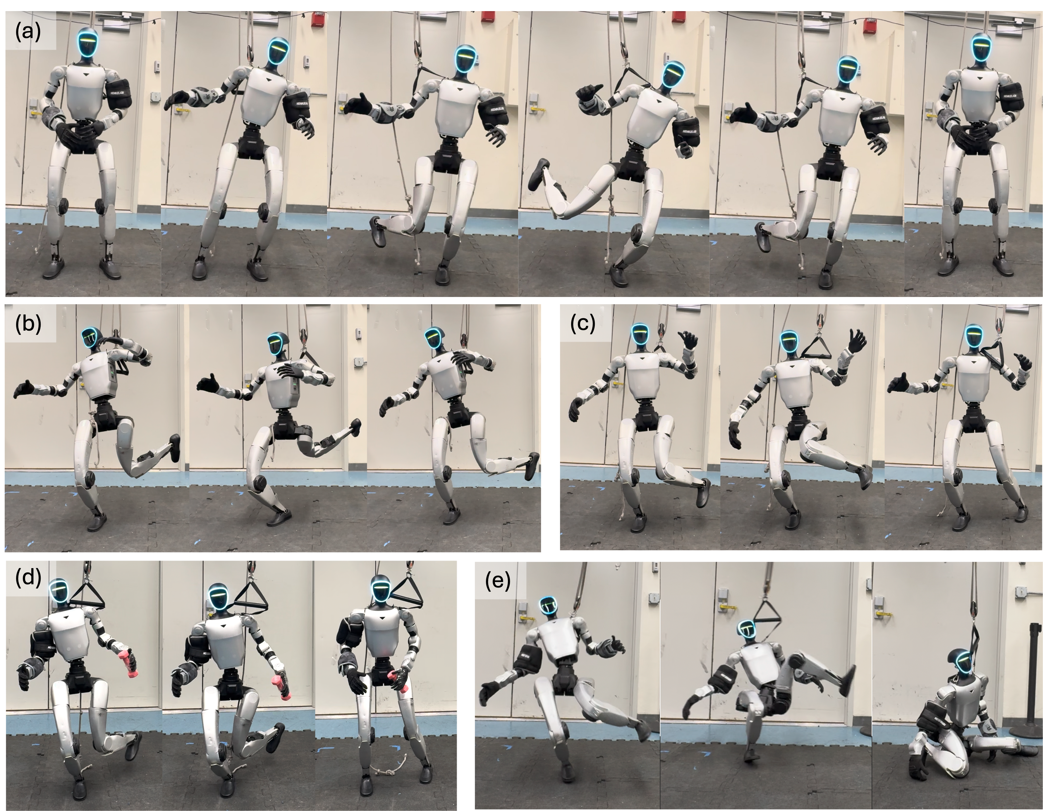
At a glance
ResSafe freezes a task-tracking policy and trains a second policy to add small action corrections that prolong safe operation. Simulation and G1 hardware experiments show improved balance under disturbances, with trade-offs in tracking accuracy. The residual resembles a minimum-change safety filter, but has no certified invariant set or hard safety guarantee. Its demonstrated transfer is across balance motions and reference-policy checkpoints within the training setup, not arbitrary humanoid tasks.
1 Introduction
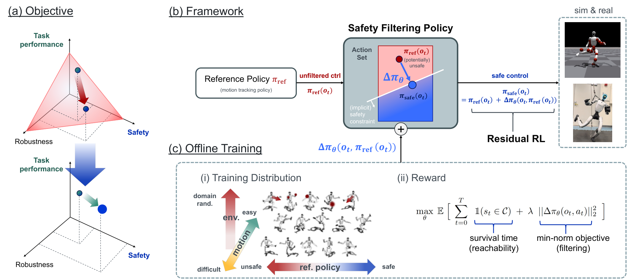
Tracking accuracy, robustness, and fall avoidance can conflict when optimized in one policy. ResSafe separates task learning from a residual correction stage, aiming to improve the empirical trade-off without online optimization. This design reduces interference between objectives but does not eliminate reward weights, domain randomization, or conservative behavior. A universal reusable safety policy is the longer-term motivation, not an achieved guarantee.
2 Related Works
Classical control barrier functions [3] and reachability methods characterize safe actions through models and certificates. Learning-based methods can instead approximate safety quantities, while residual RL modifies an existing controller. ResSafe connects these strands by learning the correction directly and compares against discriminating-hyperplane filtering [25]. The theoretical filtering framework provides motivation; its exact guarantees do not automatically transfer to a neural residual trained from samples.
3 Background & Problem Formulation
The background formulates safety as remaining inside a state constraint set. A reachability value function characterizes the maximal controlled-invariant subset, and a minimum-norm filter projects a reference action into a safe action set. For suitable control-affine settings, a discriminating hyperplane represents a half-space constraint on actions. ResSafe later replaces explicit set construction and projection with a learned correction. The retained equations describe the ideal model-based objects separately from their learned approximation.
Equations 1–9
| (1) |
| (2a) | ||||
| s.t. | (2b) | |||
| (3) |
| (4) |
| (5) |
| (6) |
| (7a) | ||||
| s.t. | (7b) | |||
| (8) |
| (9) |
Running Example (Cart-Pole).
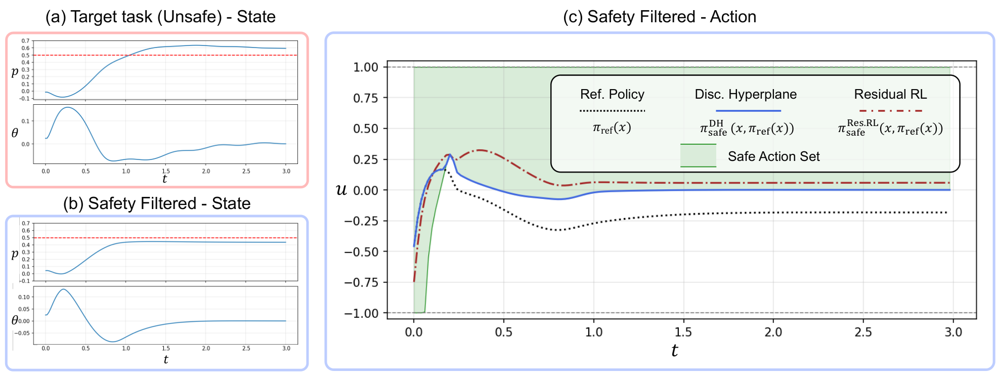
The cart-pole example deliberately conflicts: the reference controller targets cart position 0.6 while safety requires position at most 0.5. A learned hyperplane filter prevents the violation and supplies a comparison for residual corrections. The example illustrates filtering behavior in a small system; it does not establish high-dimensional humanoid guarantees.
4 Learning Safety Filtering with Residual Reinforcement Learning
The proposed method learns the additive correction itself, using survival-oriented rewards and a penalty for deviating from the nominal action.
4.1 Learning Safety Filtering with Residual RL
The residual receives state or observations together with the reference action. PPO maximizes accumulated alive reward until termination while penalizing correction magnitude. Expected survival time is a practical training objective, but by itself is not a certificate of constraint satisfaction or generally identical to maximizing full-horizon survival probability. In the cart-pole illustration, the learned correction resembles the hyperplane filter while intervening somewhat more conservatively.
Equation 10
| (10) |
4.2 Learning Safety Filters for Humanoid Balance
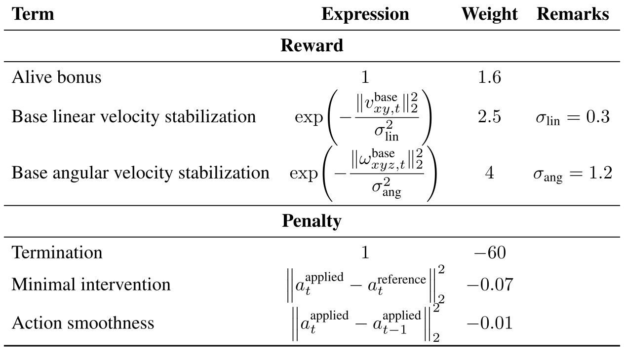
For the 29-action G1, the nominal controller follows the HuB balance-tracking pipeline [53]. A collection of 10,000 generated motions supports broader balance training. The residual adds velocity-stabilization and action-smoothness terms to survival and minimal-intervention objectives. Thus the practical reward includes several designed terms, detailed in the restored appendix table.
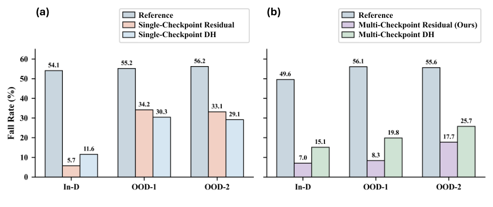
An asymmetric actor–critic gives the deployable actor proprioception and the nominal action while the critic receives privileged simulator state. Payloads and pushes expose near-failure states. Training against multiple nominal-policy checkpoints improves transfer to unseen checkpoints; training against one checkpoint can overfit its action distribution.
5 Experimental Results
The evaluation compares tracking error and fall frequency under payload disturbances, then tests checkpoint transfer and physical balance motions. The trade-off studies use one reference motion, while broader generalization and hardware studies use the motion dataset.
5.1 Experimental Setup
Baselines are the nominal tracking policy, a nominal policy trained with payload randomization, and a PPO-trained discriminating-hyperplane filter. Tracking error is measured relative to the robot base; falls provide the safety outcome. These measures assess balance in the tested scenarios, not all possible hazards such as environmental collision or unsafe contact forces.
5.2 Simulation Results
In the robustness experiment, payload fall rates are 7.29% for the nominal policy, 1.20% for randomized nominal training, and 1.11% for ResSafe. ResSafe’s payload tracking error is 37.66 mm versus 43.28 mm for randomized training. Without payload, however, the nominal policy tracks more accurately: 24.95 mm versus ResSafe’s 34.04 mm.
The separate safety-weight study shows a trade-off rather than universal dominance. ResSafe reaches 0.5% falls at 68.65 mm error; a moderate safety-penalty baseline reaches zero observed falls at 101.68 mm, while the unaugmented randomized baseline has 1.17% falls at 59.89 mm. A larger safety weight worsens both metrics. Multi-checkpoint residual training reduces degradation on held-out checkpoints compared with single-checkpoint training, within the evaluated motion-policy family.
| Policy | (w. payload) | (w/o payload) | Fall Rate (w. payload) |
| Baseline | 38.6 mm | 24.95 mm | 7.29% |
| Baseline* | 43.28 mm | 44.40 mm | 1.20% |
| ResSafe | 37.66 mm | 34.04 mm | 1.11% |
| Policy (safety-cost weight) | Fall Rate | |
| Baseline* | 59.89 mm | 1.17% |
| Baseline* + Safety (50) | 101.68 mm | 0.00% |
| Baseline* + Safety (100) | 353.55 mm | 1.63% |
| ResSafe | 68.65 mm | 0.5% |
5.3 Hardware Results
Four hardware motions are tested ten times each. ResSafe records 2/10, 1/10, 0/10, and 0/10 falls; the nominal policy records 10/10, 8/10, 10/10, and 5/10. Improvements are substantial against that baseline but mixed against the stronger alternatives. On the first payload motion, randomized nominal training has zero falls and the hyperplane filter has one, both fewer than ResSafe’s two.
Randomized nominal training also has lower tracking error than ResSafe on all four listed motions. ResSafe’s advantage is lower fall counts on three of them, especially the third and fourth payload motions. The source prose’s broad claim of outperforming every baseline in both metrics is therefore not supported uniformly by Table 3. Zero falls in ten trials is an observed sample result, not a safety guarantee.
6 Conclusion
Separating task tracking from residual correction can improve useful regions of the balance-performance trade-off and transfer to hardware. The experiments support a practical learned intervention mechanism, while explicit guarantees and broad task-independent reuse remain unresolved.
7 Limitations
The learned filter has no hard safety guarantee. Its conservative behavior lacks a complete theoretical explanation, and hardware transfer still depends on standard identification and randomization techniques. Generalization is bounded by motion-data diversity. The filter is blind to the environment beyond proprioception, so adding perception and environmental affordances is an important proposed extension.
| Method | Fall | (mm) | Method | Fall | (mm) |
| (a) #9350 (w/ payload) | (b) #1665 (w/o payload) | ||||
| Baseline | 10/10 | 84.13 12.99 | Baseline | 8/10 | 80.42 23.16 |
| Baseline* | 0/10 | 47.73 4.01 | Baseline* | 2/10 | 73.67 13.53 |
| DH | 1/10 | 67.88 20.13 | DH | 3/10 | 87.95 21.10 |
| Ours | 2/10 | 49.81 11.65 | Ours | 1/10 | 76.43 6.22 |
| (c) #6337 (w/ payload) | (d) #8407 (w/ payload) | ||||
| Baseline | 10/10 | 73.56 14.68 | Baseline | 5/10 | 75.49 28.52 |
| Baseline* | 5/10 | 62.00 14.43 | Baseline* | 2/10 | 48.49 13.62 |
| DH | 9/10 | 82.62 22.98 | DH | 4/10 | 66.10 15.04 |
| Ours | 0/10 | 70.01 3.11 | Ours | 0/10 | 61.01 4.41 |
Acknowledgments
The authors thank their discussion and hardware collaborators and acknowledge VESSL AI compute support, NSF and DARPA programs, and the UCLA Samueli School of Engineering.
Appendix A Residual Reinforcement Learning Details
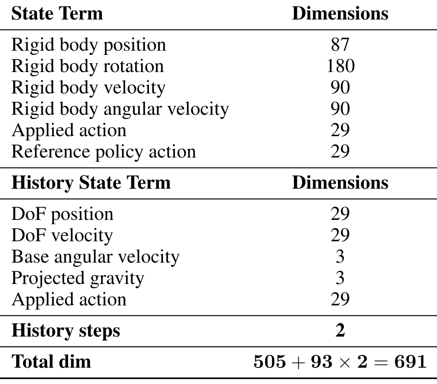
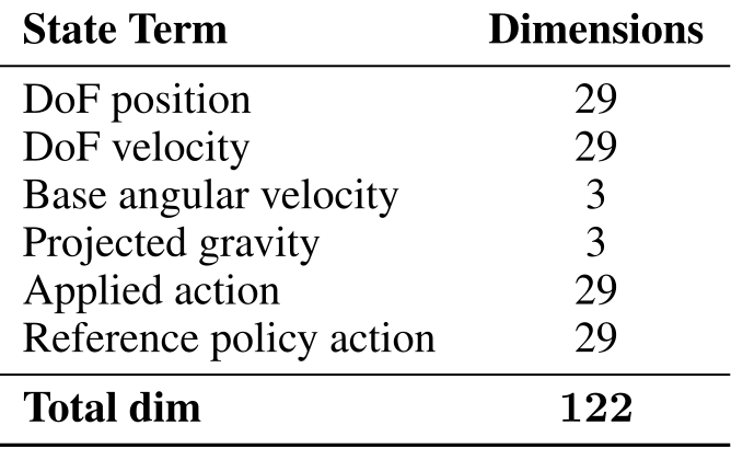
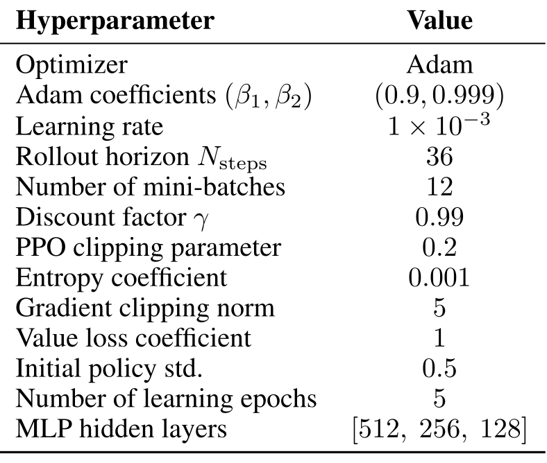
The appendix specifies the complete residual reward, actor and critic inputs, training hyperparameters, and disturbance curriculum. Tables 4–8 were absent from the source HTML except for captions and are restored below from the original PDF.
A.1 Reward Design
The practical reward weights are 1.6 for the alive bonus, 2.5 for horizontal velocity stabilization, and 4 for angular velocity stabilization, with scale parameters 0.3 and 1.2. Penalties are −60 for termination, −0.07 for squared deviation from the reference action, and −0.01 for action changes. These additional terms are important for reproducing the empirical filter and qualify the simplified survival-plus-minimum-change objective.
| Term | Expression | Weight | Remarks |
| Reward | |||
| Alive bonus | |||
| Base linear velocity stabilization | |||
| Base angular velocity stabilization | |||
| Penalty | |||
| Termination | |||
| Minimal intervention | |||
| Action smoothness | |||
A.2 State Space Design
The critic uses 691 input dimensions: privileged rigid-body state and actions plus two history steps of joint state, angular velocity, projected gravity, and applied action. The deployable actor uses 122 dimensions comprising joint positions/velocities, base angular velocity, projected gravity, applied action, and reference-policy action. The original tables retain the exact dimension breakdown.
| State Term | Dimensions |
| Rigid body position | 87 |
| Rigid body rotation | 180 |
| Rigid body velocity | 90 |
| Rigid body angular velocity | 90 |
| Applied action | 29 |
| Reference policy action | 29 |
| History State Term | Dimensions |
| DoF position | 29 |
| DoF velocity | 29 |
| Base angular velocity | 3 |
| Projected gravity | 3 |
| Applied action | 29 |
| History steps | 2 |
| Total dim |
| State Term | Dimensions |
| DoF position | 29 |
| DoF velocity | 29 |
| Base angular velocity | 3 |
| Projected gravity | 3 |
| Applied action | 29 |
| Reference policy action | 29 |
| Total dim |
A.3 Training Parameters
PPO uses an Adam learning rate of 10⁻³, a 36-step rollout, twelve minibatches, five learning epochs, discount 0.99, clipping 0.2, and entropy coefficient 0.001. The MLP hidden widths are 512, 256, and 128. Table 7 preserves the remaining optimizer, gradient, value-loss, and policy-variance settings.
| Hyperparameter | Value |
| Optimizer | Adam |
| Adam coefficients | |
| Learning rate | |
| Rollout horizon | |
| Number of mini-batches | |
| Discount factor | |
| PPO clipping parameter | |
| Entropy coefficient | |
| Gradient clipping norm | |
| Value loss coefficient | |
| Initial policy std. | |
| Number of learning epochs | |
| MLP hidden layers |
A.4 Domain Randomization
The method inherits HuB dynamics randomization and adds payloads on left/right wrists, elbows, and shoulders, with each listed link’s added mass sampled from 0–3 kg. Push velocity is sampled up to a curriculum maximum of 0.5 m/s every four seconds. The bound increases after episodes longer than 300 steps and decreases below 250 steps. This exposes the residual to challenging states while adapting disturbance severity.
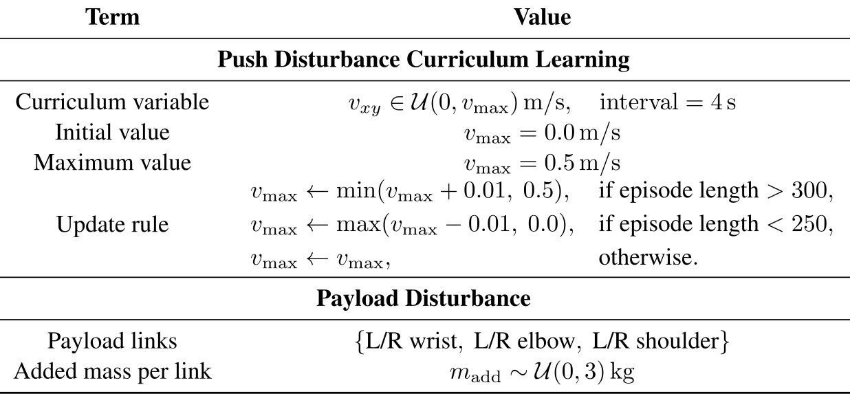
| Term | Value |
| Push Disturbance Curriculum Learning | |
| Curriculum variable | |
| Initial value | |
| Maximum value | |
| Update rule | |
| Payload Disturbance | |
| Payload links | |
| Added mass per link | |
Appendix B Experimental Details
Experimental details distinguish privileged single-motion trade-off studies from the deployable student-policy generalization and hardware setup.
B.1 Performance–Robustness Trade-off
The robustness trade-off uses one motion and the teacher reference policy to avoid distillation confounds. Both actor and critic receive the privileged Table 5 state representation in this study. It should therefore not be treated as identical to the limited-observation hardware actor.
B.2 Performance–Safety Trade-off
The safety-weight study likewise uses a single motion, the teacher reference policy, and the Table 5 input for both actor and critic. This isolates the reward/training comparison within that controlled setting.
B.3 Generalization Across Different Reference Policies
Checkpoint generalization uses the student general reference policy and full motion dataset. The purpose is transfer across controller checkpoints and a broader balance-motion distribution, rather than a change to an unrelated task family.
B.4 Hardware Results
Hardware policies are trained with the student general reference controller on the full motion dataset and tested on different motions from that dataset. These tests demonstrate sim-to-real execution within the studied motion domain, not held-out task-family generalization.