DSEI compresses both prompts and outputs into semantic segments and predicts in latent space. Its DSAE encoder combines static and task-dependent features. On English Wanjuan data with OPT backbones, the authors report up to 48% lower perplexity than sentence-level latent inference. The experiments measure language reconstruction and throughput; they do not establish broad reasoning improvements.
1 Introduction
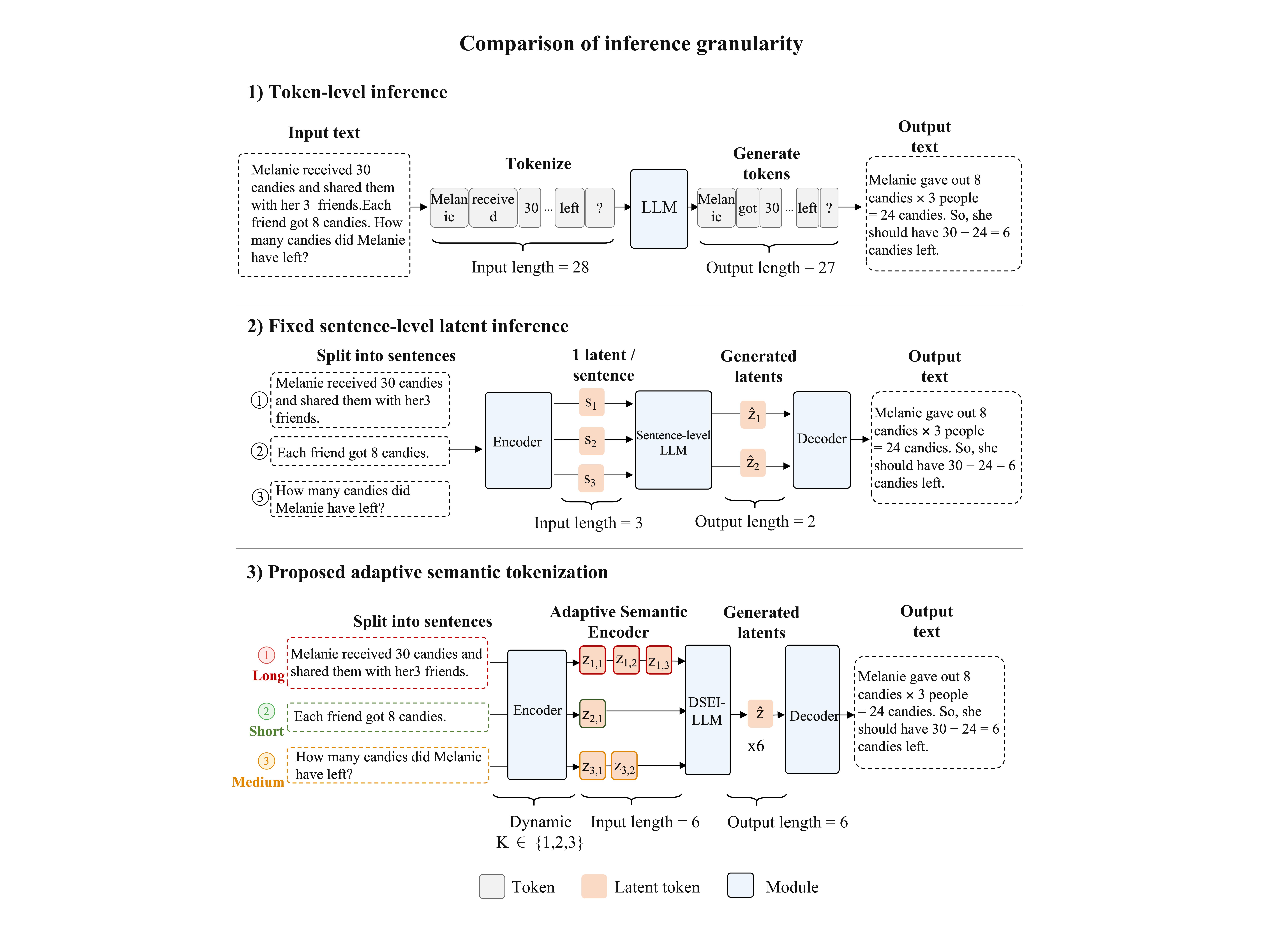
Token-by-token generation incurs long sequences and repeated computation. Compressing only intermediate reasoning leaves input and output costs intact. DSEI instead compresses the full sequence, balancing shorter latent sequences against the information lost when a long sentence becomes one vector.
Figure 1: Comparison of token-level inference, fixed sentence-level latent inference, and the proposed dynamic segment-level latent inference. DSEI segments sentences according to token length and extracts compact semantic representations based on token-level importance, reducing both input and output sequence lengths while maintaining semantic fidelity.
2 Related Work
Prior work explores semantic compression and reasoning in continuous representations.
2.1 Semantic compression
Semantic autoencoders can replace token sequences with compact vectors, but fixed sentence-level compression struggles with long or information-rich sentences. DSAE adapts segment count to sentence length and combines a static feature with attention-weighted dynamic features.
Latent reasoning methods often focus on internal chains of thought. DSEI extends compression across input and output and adds explicit segment-boundary and stopping predictions so generated representations can be decoded into text.
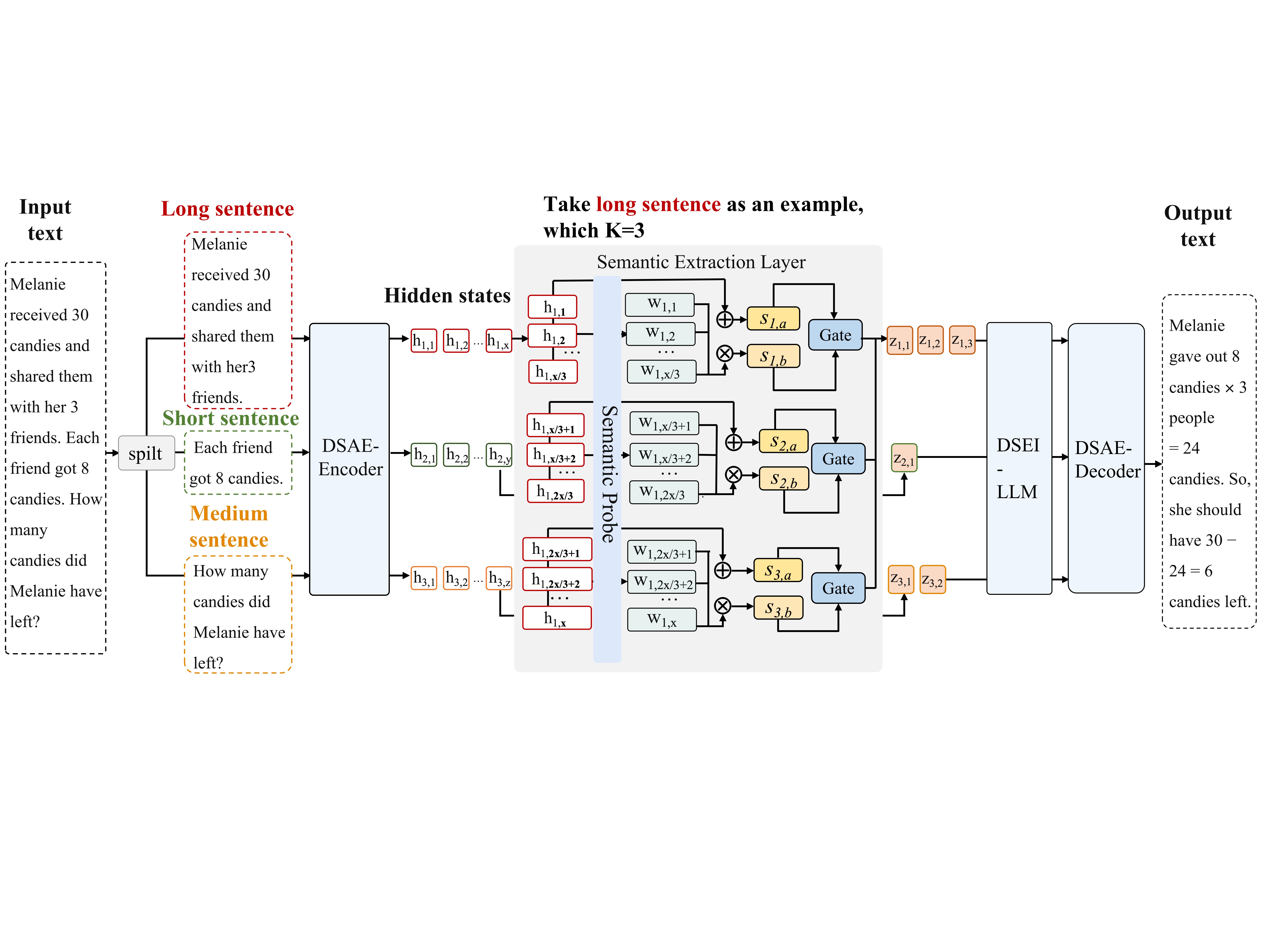
The system first trains a semantic autoencoder, then trains a latent autoregressive model with that encoder and decoder. Figure 2 shows both stages.
Figure 2: Overall architecture of the proposed DSEI framework. The input text is first split into sentences, and each sentence is partitioned into one or more segments according to token length. The DSAE encoder extracts segment-level latent representations through token-level semantic weighting and gated fusion. These latent representations are then processed by the DSEI-LLM for latent-space inference, and the generated latent outputs are reconstructed into natural language by the DSAE decoder.
3.1 Semantic Autoencoder
Sentences shorter than 15 tokens use one segment; those with 15–30 tokens use two; longer sentences use three. A learned semantic probe weights token features. A sigmoid gate combines the weighted dynamic feature and static feature before normalization. The decoder reconstructs each sentence with cross-attention to its segment vectors and a focal reconstruction loss. Encoder and decoder attention weights initialize from early and late OPT layers, respectively.
The language model predicts the next segment representation rather than the next token. A boundary head groups generated segments into sentences, and a stopping head runs at sentence boundaries. Training jointly optimizes token reconstruction, segment boundaries, and termination, with auxiliary weights of 0.01. This keeps the complete input–output process in the compressed representation until decoding.
Training uses the English portion of Wanjuan 1.0: 155 million sentences for DSAE and 6.4 million paragraphs for DSEI, with 1,000 validation examples each. Backbones are OPT-125M, OPT-350M, and OPT-1.3B. Runs use an RTX 5880 Ada, AdamW, gradient clipping, and 5,000 warmup steps. Sentence and paragraph stages use different batch sizes and learning rates; results are specific to this setup.
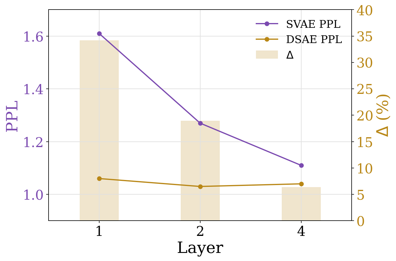
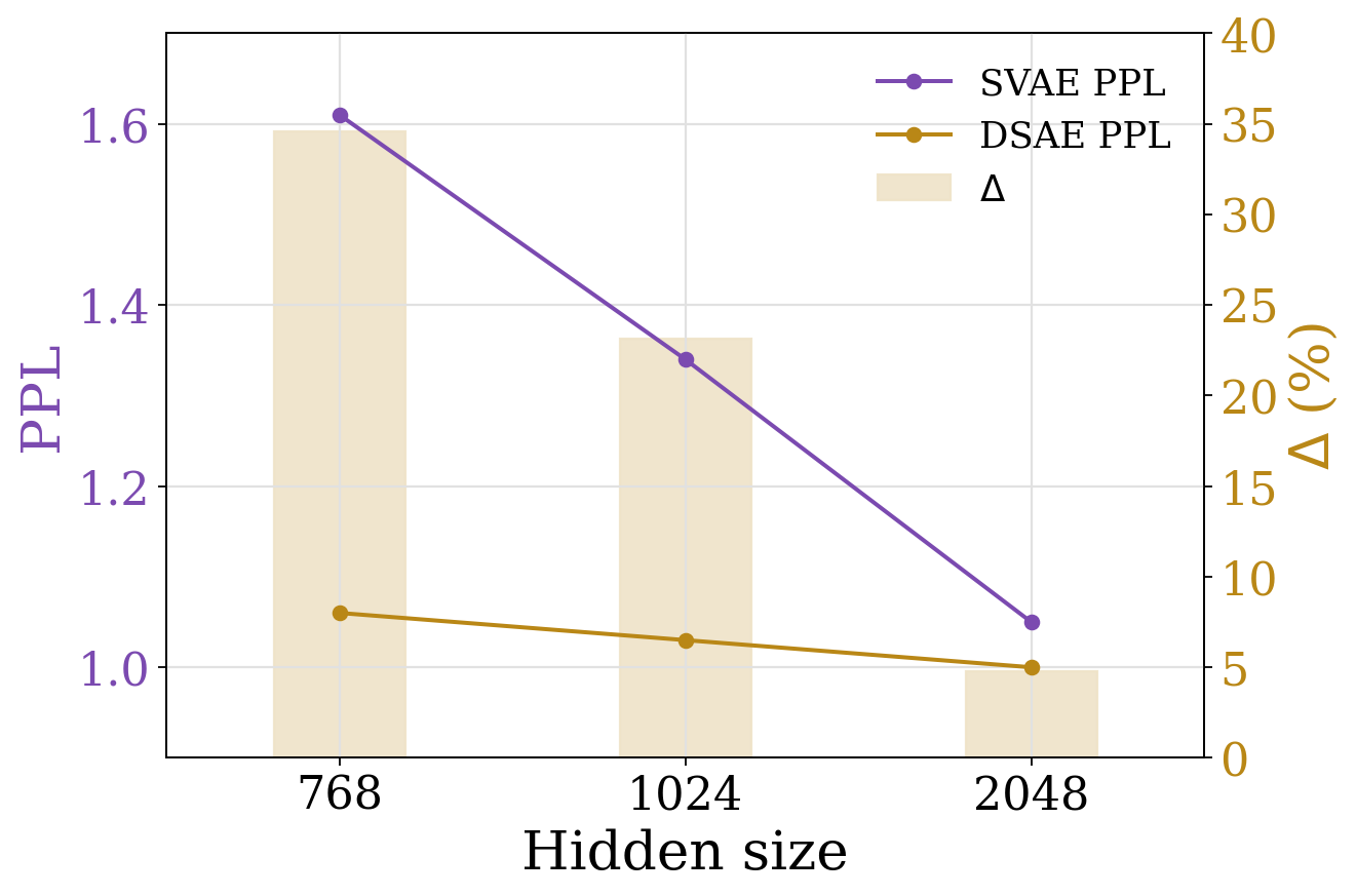
DSAE reduces perplexity by up to 34% relative to SVAE. Removing dynamic segmentation raises perplexity by about 32%; replacing the gate with a simple sum raises it by 14%. Random initialization raises it by 17%. Attention maps and decoded examples illustrate retained semantics, while Table 2 isolates the contribution of each design choice.
Figure 3: Comparison of PPL for semantic extraction between DSAE and baseline method across varying (a) layers and (b) hidden sizes. denotes percentage decrease in PPL of DSAE compared to the baseline method.
Table 1: Test examples of sentence reconstruction between baseline method and DSAE. The darker the color, the greater the weight of the token. Text in red denotes mismatches between reconstructed sentence and input sentence, and denotes missing output.
Table 2: The ablation experiment results of DSAE. denotes percentage increase in PPL compared to the default setting. “First layer weights” indicates that the initial parameters for both the encoder and the decoder are transferred from the first layer of the base LLM, while “Last layer weights” are derived from the final layer.
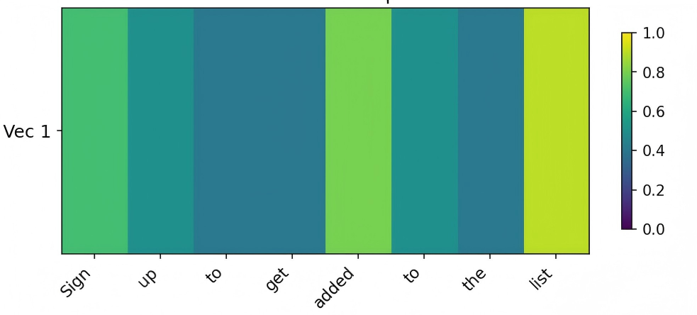
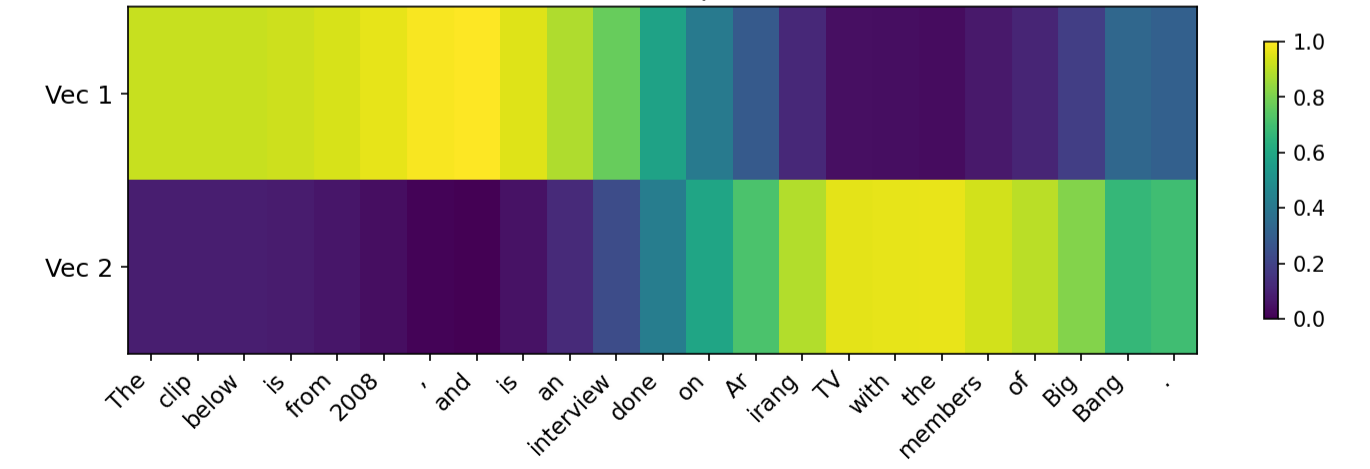
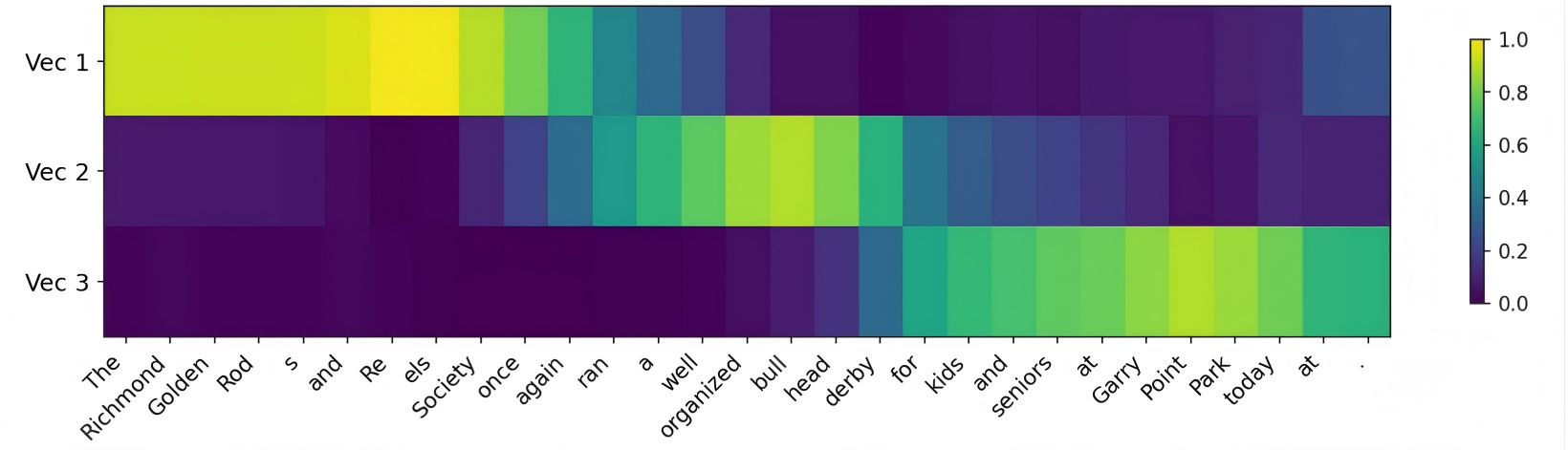
Figure 4: Attention heatmap comparison of decoder cross-attention weights on DSAE tokens for (a) short, (b) middle, and (c) long sentences during semantic compression. Lighter colors indicate higher attention weights, signifying that the decoder assigns greater importance to those tokens when reconstructing the original sentence.
4.3 Latent inference results
DSEI reports up to 48% lower perplexity than SLLM and, against token-level OPT, about 2.5× throughput, 90% lower memory, and 58% lower perplexity. These are the paper’s input-throughput and reconstruction measurements. Against SLLM at 125M scale, throughput improves only 0.22% and memory increases 18%; the additional components add roughly 0.6 million parameters. The advantage depends on the comparison and model scale.
Table 3: Experiment results of baseline methods and DSEI. DSEI-b-l denotes an OPT model with parameter size b, integrated with a DSAE consisting of l layers.
Adaptive semantic segments improve the reconstruction–compression tradeoff in the tested models. The evidence is limited to one training corpus and relatively small OPT backbones; downstream task accuracy and larger-scale deployment remain open questions.
43 references
[1]H. An, Y. Chen, Z. Sun, and X. Li (2024)Sentencevae: enable next-sentence prediction for large language models with faster speed, higher accuracy and longer context.
arXiv preprint arXiv:2408.00655.
[2]T. Cai, Y. Li, Z. Geng, H. Peng, J. D. Lee, D. Chen, and T. Dao (2024)Medusa: simple llm inference acceleration framework with multiple decoding heads.
In ICML,
[3]X. Chen, Z. Sun, G. Wenjin, M. Zhang, Y. Chen, Y. Sun, H. Su, Y. Pan, D. Klakow, W. Li, et al. (2025)Unveiling the key factors for distilling chain-of-thought reasoning.
In ACL,
[4]Y. Chen, J. Shang, Z. Zhang, et al. (2025)Inner thinking transformer: leveraging dynamic depth scaling to foster adaptive internal thinking.
In ACL,
[5]Z. Chen, A. May, R. Svirschevski, Y. Huang, M. Ryabinin, Z. Jia, and B. Chen (2024)Sequoia: scalable, robust, and hardware-aware speculative decoding.
arXiv preprint arXiv:2402.12374.
[7]Y. Deng, Y. Choi, and S. Shieber (2024)From explicit cot to implicit cot: learning to internalize cot step by step.
arXiv preprint arXiv:2405.14838.
[8]H. Du, Y. Dong, and X. Ning (2025)Latent thinking optimization: your latent reasoning language model secretly encodes reward signals in its latent thoughts.
arXiv preprint arXiv:2509.26314.
[12]S. Goyal, Z. Ji, A. S. Rawat, A. K. Menon, S. Kumar, and V. Nagarajan (2023)Think before you speak: training language models with pause tokens.
arXiv preprint arXiv:2310.02226.
[13]S. Hao, S. Sukhbaatar, D. Su, X. Li, Z. Hu, J. Weston, and Y. Tian (2025)Training large language models to reason in a continuous latent space.
In COLM,
[14]C. He, Z. Jin, C. Xu, J. Qiu, B. Wang, W. Li, et al. (2023)Wanjuan: a comprehensive multimodal dataset for advancing english and chinese large models.
arXiv preprint arXiv:2308.10755.
[24]A. Mohtashami, M. Pagliardini, and M. Jaggi (2025)CoTFormer: a chain of thought driven architecture with budget-adaptive computation cost at inference.
In ICLR,
[29]A. Shabalin, V. Meshchaninov, E. Chimbulatov, et al. (2025)Tencdm: understanding the properties of the diffusion model in the space of language model encodings.
In AAAI,
[31]D. Su, H. Zhu, Y. Xu, J. Jiao, Y. Tian, and Q. Zheng (2025)Token assorted: mixing latent and text tokens for improved language model reasoning.
In ICML,
[32]J. Tack, J. Lanchantin, J. Yu, A. Cohen, I. Kulikov, J. Lan, S. Hao, Y. Tian, J. E. Weston, and X. Li (2025)LLM pretraining with continuous concepts.
In NeurIPS,
[33]W. Tan, J. Li, J. Ju, Z. Luo, R. Song, and J. Luan (2025)Think silently, think fast: dynamic latent compression of llm reasoning chains.
arXiv preprint arXiv:2505.16552.
[35]X. Wei, X. Liu, Y. Zang, X. Dong, Y. Cao, J. Wang, X. Qiu, and D. Lin (2025)SIM-cot: supervised implicit chain-of-thought.
arXiv preprint arXiv:2509.20317.
[37]T. Wu, Z. Fan, X. Liu, H. Zheng, Y. Gong, J. Jiao, J. Li, J. Guo, N. Duan, W. Chen, et al. (2023)Ar-diffusion: auto-regressive diffusion model for text generation.
NeurIPS.
[38]J. Xu, M. Zhou, W. Liu, H. Liu, S. Han, and D. Zhang (2025)TwT: thinking without tokens by habitual reasoning distillation with multi-teachers’ guidance.
arXiv preprint arXiv:2503.24198.
[39]J. Ye, S. Gong, L. Chen, L. Zheng, J. Gao, H. Shi, C. Wu, X. Jiang, Z. Li, W. Bi, et al. (2024)Diffusion of thought: chain-of-thought reasoning in diffusion language models.
NeurIPS.
[40]H. Yuan, Z. Yuan, C. Tan, F. Huang, and S. Huang (2022)Seqdiffuseq: text diffusion with encoder-decoder transformers.
arXiv preprint arXiv:2212.10325.
[41]B. Zeng, S. Song, S. Huang, Y. Wang, H. Li, Z. He, X. Wang, Z. Li, and Z. Lin (2025)Pretraining language models to ponder in continuous space.
arXiv preprint arXiv:2505.20674.
[42]S. Zhang, S. Roller, N. Goyal, M. Artetxe, M. Chen, S. Chen, C. Dewan, M. Diab, X. Li, X. V. Lin, et al. (2022)Opt: open pre-trained transformer language models.
arXiv preprint arXiv:2205.01068.
[43]Y. Zhang, J. Gu, Z. Wu, S. Zhai, J. Susskind, and N. Jaitly (2023)Planner: generating diversified paragraph via latent language diffusion model.
NeurIPS.